Algos Prep
※ 1. Abstract
This is a running document that hosts my learnings from doing algorithmic puzzles. The main objective here is to gain an intuition for different question types so that I can pattern-match easily. This will be helpful for both technical interviews and on the daily, where identifying common patterns helps find nifty solutions to problems.
We shall explore the breadth of problems by following some common question-sets and then we can surgically tackle areas that I find non-intuitive and get some depth gains .

Table of Contents
- 1. Abstract
- 2. Tackling the Basics: Neetcode 150
- 2.1. Goals, Context and Retro
- 2.2. Arrays & Hashing
- 2.2.1. [1] Contains Duplicate (217)
- 2.2.2. [2] Valid Anagram (242)
- 2.2.3. [3] Two Sum (1)
- 2.2.4. [4] Group Anagrams (49)
- 2.2.5. [5] Top K Frequent Elements (347)
- 2.2.6. [6] Encode and Decode Strings [neetcode ref] [ref
- 2.2.7. [7] Product of Array Except Self (238)
- 2.2.8. [8] Valid Sudoku (36)
- 2.2.9. [9] Longest Consecutive Sequence (128) med sequence accumulation
- 2.2.10. [Depth-1] Subarray Sum Equals K (560) prefix_sum
- 2.2.11. [exposure-1] Sort Vowels in a String (2785)
- 2.3. Two Pointers
- 2.4. Stack
- 2.4.1. General Notes
- 2.4.2. [15] Valid Parentheses (20)
- 2.4.3. [16] Min Stack (155)
- 2.4.4. [17] Evaluate Reverse Polish Notation (150)
- 2.4.5. [18] ⭐️ Generate Parentheses (22) med redo backtracking combinations
- 2.4.6. [19] Daily Temperatures (739) med redo monotonic_stack
- 2.4.7. [20] Car Fleet (853) merge_from_one_side grouping segmentation
- 2.4.8. [21] ⭐️Largest Rectangle in Histogram (84) hard redo monotonic_stack
- 2.4.9. [Depth Blind 1] Remove Duplicate Letters (316) failed greedy monotonic_stack
- 2.4.10. [Depth-Blind 2] 132 Pattern (456) failed subsequence stack
- 2.5. Binary Search
- 2.5.1. General Notes
- 2.5.2. [22] Binary Search (704)
- 2.5.3. [23] Search a 2D Matrix (74) custom_flattening
- 2.5.4. [24] Koko Eating Bananas (875)
- 2.5.5. [25] Find Minimum in Rotated Sorted Array (153) almost
- 2.5.6. [26] Time Based Key Value Store (981)
- 2.5.7. TODO [27] Median of two sorted arrays [4] redo hard binary_search median virtual_domain
- 2.5.8. [Depth 1] Capacity to Ship Packages within D Days (1011) left_boundary_finding binary_search
- 2.5.9. [Depth 2] Find Minimum in Rotated Sorted Array II (154) hard binary_search rotated_array
- 2.5.10. [Depth 3] Search in Sorted Array (33) med
- 2.5.11. [Exposure 1] First/Last Position of Element in Sorted Array (34)
- 2.5.12. [Exposure 2] Single Element in a Sorted Array (540)
- 2.6. Sliding Window
- 2.6.1. General Notes
- 2.6.2. [28] Best Time to Buy And Sell Stock (121) sliding_window converge_to_a_side kadane_light
- 2.6.3. [29] Longest Substring Without Repeating Characters (3) sliding_window
- 2.6.4. [30] Longest Repeating Character Replacement (424) redo
- 2.6.5. [31] Permutation in String (567)
- 2.6.6. [32] Minimum Window Substring (76) hard almost
- 2.6.7. [33] Sliding Window Maxiumum (239) hard monotonic_deque
- 2.6.8. [Depth-Blind 1] Maximum Number of Vowels in a Substring of Given Length (1456) sliding_window
- 2.6.9. [Depth-Blind 2] Replace the Substring for Balanced String (1234) failed almost character_counting
- 2.6.10. [Depth-Blind 3] Find all Anagrams in a String (438) char_counting sliding_window fixed_size
- 2.6.11. TODO [Depth-Blind 3] Subarrays with K different Integers (992) failed double_window
- 2.6.12. [Exposure 1] Number of People Aware of a Secret (2327)
- 2.7. Linked List
- 2.7.1. General Notes
- 2.7.2. [34] Reverse Linked List (206)
- 2.7.3. [35] Merge Two Sorted Lists (21) dummy_node_method
- 2.7.4. [36] Linked List Cycle (141) tortoise_hare_method
- 2.7.5. [37] Reorder List (143) in_place split_reverse_merge_method
- 2.7.6. [38] Remove Nth Node from End of List (19) med dummy_node_method
- 2.7.7. [39] Copy List with Random Pointer (138) interleaving_method
- 2.7.8. [40] Add two numbers (2) dummy_node_method human_calculation
- 2.7.9. [41] ⭐️ Find the Duplicate Number (287) redo tortoise_hare_method array linked_list
- 2.7.10. [42] LRU Cache (146)
- 2.7.11. [43] Merge k sorted lists [23] hard merge_sort_merge_method min_heap
- 2.7.12. [44] Reverse nodes in k-Group (25) redo almost hard dummy_node_method sliding_window
- 2.7.13. [Depth-1] Swap Nodes in Pairs (24)
- 2.8. Trees
- 2.8.1. General Notes
- 2.8.2. [45] Invert Binary Tree (226)
- 2.8.3. [46] Maximum Depth of Binary Tree (104)
- 2.8.4. [47] Diameter of Binary Tree (543) redo post_order_dfs easy
- 2.8.5. [48] Balanced Binary Tree (110) state_threading
- 2.8.6. [49] Same Tree (100)
- 2.8.7. [50] Subtree of Another Tree (572) sameness
- 2.8.8. [51] Lowest Common Ancestor of a Binary Search Tree (235) BST
- 2.8.9. [52] Binary Tree Level Order Traversal (102)
- 2.8.10. [53] Binary Tree Right Side View (199) right_first_traversal
- 2.8.11. [54] Count Good Nodes in Binary Tree (1448)
- 2.8.12. [55] Validate Binary Search Tree (98) bst_property
- 2.8.13. [56] Kth Smallest Element in BST (230) augmentation
- 2.8.14. [57] ⭐️ Construct Binary Tree from Preorder and Inorder Traversal (105) redo traversal_properties
- 2.8.15. [58] Binary Tree Maximum Path Sum (124) redo hard gain_accumulation
- 2.8.16. TODO [59] Serialize and Deeserialize Binary Tree (297) redo hard backtracking trie
- 2.8.17. [Depth 1] Lowest Common Ancestor of a Binary Tree (236)
- 2.9. Tries
- 2.10. Backtracking
- 2.10.1. General Notes
- 2.10.2. [63] ⭐️ Subsets (78) redo power_set combinations no_duplicates_allowed
- 2.10.3. [64] Combination Sum (39) redo combination duplicates_allowed
- 2.10.4. [65] Combination Sum II (40) redo almost permutation pruning mental_model_clearer_now
- 2.10.5. [67] Permutations (46) permutation
- 2.10.6. [68] Subsets II (90) pruning combination
- 2.10.7. [69] Word Search (79) DFS
- 2.10.8. [70] Palindrome Partitioning (131) almost partitioning pruning
- 2.10.9. [71] Letter Combinations of a Phone Number (17)
- 2.10.10. [72] ⭐️ N-Queens (51) hard almost redo pruning board matrix chess
- 2.10.11. [Depth-1] Sudoku Solver (37) hard sudoku dimension_flattening_index
- 2.11. Heap / Priority Queue
- 2.11.1. General Notes
- 2.11.2. [73] Kth Largest Element in a Stream (703)
- 2.11.3. [74] Last Stone Weight (1046)
- 2.11.4. [75] K Closest Points to Origin (973)
- 2.11.5. [76] ⭐️ Kth Largest Element in an Array (215) redo quick_select_algo
- 2.11.6. [77] Task Scheduler (621) almost redo greedy priority_queue
- 2.11.7. [78] Design Twitter (355) K_way_merge
- 2.11.8. [79] Find Median from Data Stream (295) hard double_heap_method
- 2.12. Graphs
- 2.12.1. General Notes
- 2.12.2. [80] Number of Islands (200) flood_fill reuse_input union_find
- 2.12.3. [81] Max Area of Island (695) flood_fill
- 2.12.4. [82] Clone Graph (133) BFS undirected_graph almost
- 2.12.5. [83] Walls and Gates (??) multi_source_BFS
- 2.12.6. [84] Rotting Oranges (994) multi_source_BFS simulated_time_frontier
- 2.12.7. [85] ⭐️ Pacific Atlantic Water Flow (417) complement_approach flood_fill simulation border_to_center inverse_requirements reachability
- 2.12.8. [86] Surrounded Regions (130) bad_question complement_approach intermediate_marks border_to_center
- 2.12.9. [87] Course Schedule I (207) redo 3_state_visited Kahns_algo topological_sort cycle_detection
- 2.12.10. [88] Course Schedule II (210) Kahn_algo topological_sort
- 2.12.11. [89] Graph Valid Tree (??)
- 2.12.12. [90] Number of Connected Components in an Undirected Graph (323) union_find
- 2.12.13. [91] ⭐️ Redundant Connection (684) redo union_find cycle_finding incremental_processing
- 2.12.14. [92] Word Ladder (127) hard almost wildcard_pattern_matching
- 2.12.15. [D-1] Is Graph Bipartite (785) bipartite_graph
- 2.12.16. [D-2] Possible Bipartition (886) bipartite_graph
- 2.13. 1-D DP
- 2.13.1. General Notes
- 2.13.2. [93] Climbing Stairs (70)
- 2.13.3. [94] Min Cost Climbing Stairs (746) cost_reference rolling_2_var_method
- 2.13.4. [95] House Robber I (198)
- 2.13.5. [96] House Robber II (213) circular_dependencies number_of_subproblems
- 2.13.6. [97] ⭐️ Longest Palindromic Substring (5) 2D_DP Manachers_Algo
- 2.13.7. [98] Palindromic Substrings (647) 2D_DP
- 2.13.8. [99] Decode Ways (91) redo 1D_DP rolling_2_var_method
- 2.13.9. [100] Coin Change (322) DP recursive_top_down
- 2.13.10. [101] Maximum Product Subarray (152) redo rolling_2_var_method 1D_DP
- 2.13.11. [102] Word Break (139) 1D_DP 2_pointers
- 2.13.12. [103] Longest Increasing Subsequence (300) 1D_DP patience_tracking_algo
- 2.13.13. [104] ⭐️ ⭐ Partition Equal Subset Sum 1D_DP 0_1_subset_sum 0_1_knapsack knapsack counting_dp counting
- 2.13.14. [Depth Blind 1] Ones and Zeroes (474) failed 0_1_subset_sum knapsack
- 2.13.15. TODO [Depth-Blind 2] Tallest Billboard (956) failed balanced_partition knapsack
- 2.14. Intervals
- 2.14.1. General Notes
- 2.14.2. [105] Insert Interval (57)
- 2.14.3. [106] Merge Intervals (56)
- 2.14.4. [107] Non-Overlapping Intervals (435) redo greedy sort_end_times
- 2.14.5. [108] Meeting Rooms I (???)
- 2.14.6. [109] Meeting Rooms II (???)
- 2.14.7. [110] Minimum Interval to Include Each Query (1851) almost hard 2_pointers min_heap
- 2.14.8. [exposure-1] Find the Number of Ways to Place People II (3027) hard sweepline
- 2.15. Greedy Algos
- 2.15.1. General Notes
- 2.15.2. [111] Maximum Subarray (53) greedy kadane_algorithm
- 2.15.3. [112] Jump Game (55) greedy
- 2.15.4. [113] Jump Game II (45) greedy rephrase_the_question
- 2.15.5. [114] Gas Station (134) redo greedy kadane_algorithm
- 2.15.6. [115] Hand of Straights (846) almost greedy frequency_counting
- 2.15.7. [116] Merge Triplets to Form Target Triplet (1899) almost element_wise_max coverage_check
- 2.15.8. ⭐️ [117] Partition Labels (763)
- 2.15.9. [118] Valid Parenthesis String (678) 2_stack greedy_range_counting
- 2.15.10. [Exposure-1] Minimum Number of People to Teach (1733) counting disguised_as_graph
- 2.16. Advanced Graphs
- 2.16.1. General Notes
- 2.16.2. [119] Network Delay Time (743) dijkstra single_source_to_all_dest
- 2.16.3. [120] ⭐️Reconstruct Itinerary (332) hard Eulerian_path excusemewhat Heirholzers_algo
- 2.16.4. [121] Min Cost to Connect All Points (1584) space_hacking lazy_hack lazy Prims_algo
- 2.16.5. [122] ⭐️ Swim in Rising Water (778) hard flood_fill dijkstra binary_search
- 2.16.6. [123] ⭐️ Alien Dictionary (269) redo tedius hard Kahns_algo topological_sort
- 2.16.7. [124] Cheapest Flights Within K Stops (787) bellman_ford almost confounding_gotcha
- 2.16.8. [Depth-Blind] Sort Items by Groups Respecting Dependencies (1203) failed 2_phase_topological_sort topological_sorting
- 2.17. 2-D DP
- 2.17.1. General Notes
- 2.17.2. [125] Unique Paths (62) path_enum DP combinatorial_solution
- 2.17.3. [126] Longest Common Subsequence (1143) classic string_dp prefix_tracking
- 2.17.4. [127] ⭐️ Best Time to Buy and Sell Stock with Cooldown (309) state_machine FSM_DP n_array_dp time_simulation snapshot_rolling_vars
- 2.17.5. [128] ⭐️⭐️ Coin Change II (518) redo 1D_DP combination_sum combinations unbounded_knapsack knapsack counting
- 2.17.6. [129] ⭐️⭐️ Target Sum (494) problem_reduction bounded_knapsack knapsack subset_sum 1D_DP backward_loop_trick
- 2.17.7. DONE [130] Interleaving String (97) interleaving rolling_1D_array
- 2.17.8. ⭐️ [132] Distinct Subsequences (115) hard subsequences dp
- 2.17.9. [133] Edit Distance (72) subsequences prefix_matching
- 2.17.10. [134] ⭐️ Burst Balloons (312) redo hard interval_DP divide_and_conquer think_in_reverse matmul_dp_pattern
- 2.17.11. DONE [135] Regular Expression Matching (10) hard regex_matching 2D_string_matching
- 2.17.12. [Depth Blind 1] Word Break II (140) hard failed
- 2.17.13. [Depth Blind 2] Number of Unique Good Subsequences (1987) hard failed counting 2_state_tracking
- 2.18. Bit Manipulation
- 2.18.1. General Notes
- 2.18.2. [136] Single Number (136) classic pair_cancellation_via_XOR
- 2.18.3. [137] Number of 1 Bits (191) hamming_weight popcount
- 2.18.4. [138] Counting Bits (338) DP popcount
- 2.18.5. [139] Reverse Bits (190) bit_reversal fixed_width
- 2.18.6. [140] Missing Number (268) pair_cancellation_via_XOR compare_with_idx
- 2.18.7. [141] ⭐️Sum of Two Integers (371) sum_without_operator fixed_width_integer
- 2.18.8. [142] ⭐️Reverse Integer (7) overflow_detection decimal_shift
- 2.19. Math & Geometry
- 2.19.1. General Notes
- 2.19.2. [143] Rotate Image (48) redo pointer_management matrix_rotation
- 2.19.3. [144] Spiral Matrix (54) redo accuracy_problem pointer_management direction_simulation
- 2.19.4. [145] Set Matrix Zeroes (73) in_place_markers
- 2.19.5. [146] Happy Number (202) tortoise_hare_method integer_division_vs_float_division test_for_loop
- 2.19.6. [147] Plus One (66) carry_propagation in_place
- 2.19.7. [148] Pow(x, n) (50) redo fast_exponentiation binary_exponentiation classic
- 2.19.8. [149] ⭐️ Multiply Strings (43) multiplication_algo
- 2.19.9. [150] Detect Squares (2013) cartesian_plane
- 2.19.10. [exposure-1] Alice and Bob Playing Flower Game (3021) counting
- 2.19.11. [exposure-2] Sort Matrix by Diagonals (3446)
- 2.19.12. [exposure-3] Walking Robot Simulation (874) simulation turtlebot
- 3. Depth Gains
- 4. Exposure Gains
- 5. Basic Grid 83 & Neetcode 150
- 5.1. Day 1
- 5.2. Day 2
- 5.3. Day 3
- 5.4. Day 4 [Restart]
- 5.4.1. [8] Lowest Common Ancestor of a Binary Search Tree (235) topic_tree
- 5.4.2. [9] Balanced Binary Tree (110) tree
- 5.4.3. [10] Linked List Cycle (141) pointers tortoise_hare_method graph cycle_detection
- 5.4.4. [11] Implement Queue Using Stacks (232) queue stack
- 5.4.5. [12] First Bad Version (278)
- 5.5. Day 5
- 5.6. Day 6
- 5.7. Day 7
- 5.8. Day 8
- 5.9. Day 9
- 5.10. Day 10
- 5.11. Day 11
- 5.11.1. [34] permutations [46] med recursion
- 5.11.2. [35] merge intervals [56] med array
- 5.11.3. TODO [36] Lowest Common Ancestor of a Binary Tree [236]
- 5.11.4. [37] Time Based Key-Value Store [981] med binary_search
- 5.11.5. [38] Minimum Window Substring [76] hard string
- 5.11.6. [39] Reverse Linked List [206] easy linked_list
- 5.11.7. [40] Serialize and Deserialize Binary Tree [297] hard binary_tree
- 5.12. Day 12
- 5.13. Day 13
- 5.14. Day 13 (restart)
- 5.15. Day 14
- 5.16. Day 15 Back from India + Revision
- 5.17. Day 16
- 5.18. Day 17
- 5.19. Day 18
- 5.20. Day 19 Restart
- 5.21. Day 20
- 5.22. Day 21
- 5.23. Day 22
- 5.24. Day 23
- 5.25. Day 24
- 5.26. Day 25
- 5.27. Day 26 started neetcode 150 hashing arrays
- 6. Personal Python Recipes & Idioms
- 7. Notes
- 8. TODOs
- 9. References
※ 2. Tackling the Basics: Neetcode 150
This should give some breadth of understanding. For each category of questions, we shall spend some time learning about the key ideas behind that category and then dive into it. Then we can tackle the weaker topics to hone the intuition, the expanded Neetcode 250 list can be found here. Then we can tackle some hard questions. Then we can finally just do randomly to let the RNG-gods give us experience.
※ 2.1. Goals, Context and Retro
-—
The labuladong blog has a really good outline of this process, in which they encourage the exploration of patterns and learning about patterns in a quality-first approach as opposed to a quantity approach. They encourage people to develop a framework for common patterns so that pattern-matching becomes easier. It’s good to read it. Careful not to be too dogmatic about frameworks though, the important thing is to still get the intuition behind things, we never were good at memory-work anyway.
-—
The time reports for the sections are for doing, correcting and reviewing. Reviewing is roughly about 60-75% of the time taken.
In general, I’m targeting to reach 20 mins for mediums, less than 10 for easy, 30 mins for hards.
-—
Retro:
Now that I’ve finished this basic 150 questions, I have some learnings:
What has been good:
- I’m mostly able to get the intuition behind the questions or have an intuition for what the tricks are. It’s not really that difficult to grasp the basic concepts. The tricky ones come in typical patterns (e.g. tedium vs attention to detail that elucidates a non-obvious mathematical/logical property).
- My coding style is very clean and demonstrates the best parts about the language. So the implementation is usually performant, only possibly bottle-necked by algorithmic complexity.
- really grateful for my live website solution that is pleasant to use and assists me with the memory hacking. First thing I do when I’m up is think about what I did yesterday and what I will achieve today. Last thing I think of when I sleep is to review what I did today and what I will do tomorrow. I will be spartan about this. Motivation is high when things click easily. That’s the feeling to keep driving my confidence upwards.
What needs improvement:
- I haven’t been successfully able to build up incrementally to the Hard solutions. I believe that this is making me subconsciously think that the hard questions are just straight up pedantic / test for something only luck will help. I would like to NOT believe in that and find better ways to incrementally build up to optimal solutions. Honing my “Socratic thinking” would be a good way to do so. And also just straight up exposure to questions.
- I think implementation speed largely depends on how fast I come up with the v0.
- Entertaining the tests and focusing on the human aspects of face-to-face question solving. When I’m tired, I just think in my head. Additionally, the vocalisation is not efficient and it ends up distracting me sometimes. I’m usually a good teacher though, so I should probably speak in reaction to my thinking or realisation instead of multiplexing.
motivation management: spillovers have been demoralising. I think I need to do some emotional hacks and just always present the current situation as advantageous. I will have to identify the smallest to the biggest of wins for me.
Related to work-rate, I’ll just let the time-tracking guide me. When I realise that it’s only brainfog, then I need to allow myself to rest. Add variety in the activity.
How that affects the Depth Phase:
- I think my depth phase will have just two parallel goals:
personal topical weaknesses + revision of the neetcode 150 questions.
I’ll just be adding onto the topical notes at the top of every topic section, where I already have some notes.
The purpose here would be to distil the following from my existing notes from the neetcode 150 batch:
- boilerplate
- common tricks that I haven’t consolidated yet
- pitfalls: logical, accuracy / implementation.
generic topical weaknesses that usually comes up for most people.
These are the topics that people generally find difficult and which are over-represented in interviews.
- advanced graphs
- DP
- I will have to timebox the depth phase better.
※ 2.2. Arrays & Hashing
| Headline | Time | ||
|---|---|---|---|
| Total time | 3:11 | ||
| Arrays & Hashing | 3:11 | ||
| [1] Contains Duplicate (217) | 0:05 | ||
| [2] Valid Anagram (242) | 0:02 | ||
| [3] Two Sum (1) | 0:04 | ||
| [4] Group Anagrams (49) | 0:30 | ||
| [5] Top K Frequent Elements (347) | 0:28 | ||
| [7] Product of Array Except Self (238) | 0:38 | ||
| [8] Valid Sudoku (36) | 0:52 | ||
| [9] Longest Consecutive Sequence (128) | 0:32 |
※ 2.2.1. [1] Contains Duplicate (217)
Given an integer array nums, return true if any value appears at
least twice in the array, and return false if every element is
distinct.
Example 1:
Input: nums = [1,2,3,1]
Output: true
Explanation:
The element 1 occurs at the indices 0 and 3.
Example 2:
Input: nums = [1,2,3,4]
Output: false
Explanation:
All elements are distinct.
Example 3:
Input: nums = [1,1,1,3,3,4,3,2,4,2]
Output: true
Constraints:
1 <nums.length <= 10=5-10=^{=9}= <= nums[i] <= 10=9
※ 2.2.1.1. Constraints and Edge Cases
Nothing out of the ordinary here, there’s no indication of needing to handle integer overflow cases or to do any type changes.
※ 2.2.1.2. My Solution (Code)
1: class Solution: 2: │ def containsDuplicate(self, nums: List[int]) -> bool: 3: │ │ return len(set(nums)) != len(nums)
※ 2.2.1.2.1. Improved version
1: def containsDuplicate(self, nums: List[int]) -> bool: 2: │ seen = set() 3: │ for num in nums: 4: │ │ if num in seen: 5: │ │ │ return True 6: │ │ seen.add(num) 7: │ return False
This just early-exits but the asymptotic performance is the same (linear time and linear space).
※ 2.2.1.3. My Approach/Explanation
Since it’s a member duplicates check and they’re only looking for bool output, can just resort to anything that is a default stdlib function.
Size checks make sense and the only problem I can fault this for is that it requires a duplication in memory because of the creation of the set.
The size checks via len should be fast because it’s a struct-value check.
※ 2.2.1.4. My Learnings/Questions
- I should spend a little bit longer trying to entertain the edge cases if it’s an in-person thing and someone is evaluating me for my thought process. If it’s a bot, then it’s alright I can just send as I wish.
- It doesn’t have an early-exit pattern
※ 2.2.2. [2] Valid Anagram (242)
Given two strings s and t, return true if t is an anagram of
s, and false otherwise.
Example 1:
Input: s = “anagram”, t = “nagaram”
Output: true
Example 2:
Input: s = “rat”, t = “car”
Output: false
Constraints:
1 <s.length, t.length <= 5 * 10=4sandtconsist of lowercase English letters.
Follow up: What if the inputs contain Unicode characters? How would you adapt your solution to such a case?
※ 2.2.2.1. Constraints and Edge Cases
- didn’t spend much time looking into this
※ 2.2.2.2. My Solution (Code)
1: from collections import Counter 2: 3: class Solution: 4: │ def isAnagram(self, s: str, t: str) -> bool: 5: │ │ if (len(s) != len(t)): 6: │ │ │ return False 7: │ │ │ 8: │ │ return Counter(s) == Counter(t)
- the length check is an early return that makes things fast
※ 2.2.2.2.1. Improved solution
Because the constraint given is limited to the english language letters, we know that the charset is fixed (26char). Therefore, it’s even faster to just do fixed length char arrays and then do the counting:
1: class Solution: 2: │ def isAnagram(self, s: str, t: str) -> bool: 3: │ │ if len(s) != len(t): 4: │ │ │ return False 5: │ │ count = [0] * 26 6: │ │ for c1, c2 in zip(s, t): 7: │ │ │ count[ord(c1) - ord('a')] += 1 8: │ │ │ count[ord(c2) - ord('a')] -= 1 9: │ │ return all(x == 0 for x in count) 10:
※ 2.2.2.3. My Approach/Explanation
- Character counting works great if we use
collections::Counterwhich gives a refmap of the characters and their counts - The choice of DS is whether the charspace is fixed or not
- Counter works with a hashtable under the hood.
※ 2.2.2.4. My Learnings/Questions
Question: will Counter() handle different encodings well?
Answer: Yes: Counter works with any hashable object, including Unicode characters, so it will count any character in the input string, regardless of encoding
Caveat: If you want to support Unicode, your code doesn’t need to change, but using a fixed-size array for counting would not work; you must use a hash table (Counter or dict).
- Other things that Counter can be used for
- in the realm of character counting there are other approaches that might make sense:
- if the charset is known then can use a fixed array representing the charset might make sense. than can just count based on that fixed idx Datastructures for character counting:
- Using a fixed-size array for counting is the most space-efficient for lowercase English letters, as it avoids hash table overhead and is always O(1) space
- Sorting both strings and comparing them is another common approach, but it is O(nlogn)O(nlogn) and thus less efficient than counting.
For efficiently counting character frequencies, several data structures can be considered, each with its own advantages: 1. **Hash Table (Dictionary in Python)**: │ - **Time Complexity**: O(n) for counting frequencies, where n is the number of characters. │ - **Space Complexity**: O(k), where k is the number of distinct characters. │ - **Use Case**: Ideal for counting frequencies of characters or words, as it allows for constant-time complexity for insertions and lookups. This is especially useful for large datasets where you need to maintain a count of each unique character or word[2][4]. │ 2. **Counter from `collections` Module**: │ - **Time Complexity**: O(n). │ - **Space Complexity**: O(k). │ - **Use Case**: A specialized dictionary for counting hashable objects. It provides a clean and efficient way to count frequencies and is highly optimized for this purpose. It simplifies the code and is recommended for most frequency counting tasks in Python[6]. │ 3. **List (for Fixed-Size Character Sets)**: │ - **Time Complexity**: O(n). │ - **Space Complexity**: O(1) if the character set size is fixed (e.g., ASCII or lowercase English letters). │ - **Use Case**: Suitable for counting frequencies of characters when the character set is limited and known in advance. This approach uses a fixed-size list indexed by character codes, making it very efficient in terms of both time and space[2]. │ 4. **Counting Sort**: │ - **Time Complexity**: O(n + k), where k is the range of the input. │ - **Space Complexity**: O(k). │ - **Use Case**: Useful when you need to sort data based on frequency counts. It is efficient for small ranges of input values and when sorting is required based on frequency[7]. │ ### Summary For most general-purpose applications, using a `Counter` from Python's `collections` module is recommended due to its simplicity and efficiency. If you are dealing with a fixed character set, using a list to count frequencies can be slightly more efficient. For scenarios involving sorting based on frequency, counting sort can be a good choice. Citations: [1] https://stackoverflow.com/questions/74344201/appropriate-data-structure-for-counting-frequency-of-string [2] https://www.geeksforgeeks.org/counting-frequencies-of-array-elements/ [3] https://discourse.julialang.org/t/how-to-count-all-unique-character-frequency-in-a-string/19342 [4] https://users.rust-lang.org/t/efficient-string-hashmaps-for-a-frequency-count/7752 [5] https://www.sololearn.com/en/Discuss/2705816/letter-frequency-on-python-data-structures [6] https://towardsdatascience.com/3-ways-to-count-the-item-frequencies-in-a-python-list-89975f118899?gi=dcc78c14cf09 [7] https://www.geeksforgeeks.org/counting-sort/ [8] https://docs.python.org/uk/3/tutorial/datastructures.html
※ 2.2.2.4.1. Other uses of Counter
Python’s **collections.Counter** is a specialized subclass of the built-in dictionary designed for counting hashable objects. It works by storing elements as dictionary keys and their counts as values, making it easy to tally occurrences of items in iterables or mappings[4][2][5]. **How Counter Works:** - **Initialization:** You can create a Counter in several ways: │ - From an iterable (like a list or string): │ ```python │ from collections import Counter │ c = Counter(['a', 'b', 'a', 'c', 'b', 'a']) │ # Counter({'a': 3, 'b': 2, 'c': 1}) │ ``` │ - From a mapping (dictionary): │ ```python │ c = Counter({'red': 4, 'blue': 2}) │ # Counter({'red': 4, 'blue': 2}) │ ``` │ - Using keyword arguments: │ ```python │ c = Counter(red=4, blue=2) │ # Counter({'red': 4, 'blue': 2}) │ ``` │ - **Behavior:** │ - Accessing a missing key returns `0` instead of raising a KeyError[4][5]. │ - Counts can be positive, zero, or negative integers[2][5]. │ - Setting a count to zero does not remove the key; use `del` to remove it entirely[4]. │ - **Common Methods:** │ - `.elements()`: Returns an iterator over elements, repeating each as many times as its count (ignores counts less than one)[5][3]. │ - `.most_common([n])`: Returns a list of the `n` most common elements and their counts, sorted from most to least common. If `n` is omitted, returns all elements[5][3][8]. │ - `.subtract(iterable_or_mapping)`: Subtracts counts from another iterable or mapping; counts can go negative[5][3]. │ - `.update(iterable_or_mapping)`: Adds counts from another iterable or mapping[5]. │ - `.total()`: Returns the sum of all counts[5]. │ - **Arithmetic and Set Operations:** │ Counter supports addition, subtraction, intersection (`&`), and union (`|`) operations, which combine counts in intuitive ways[7]. │ **Usage Example:** ```python from collections import Counter words = ['apple', 'banana', 'apple', 'orange', 'banana', 'apple'] counter = Counter(words) print(counter) # Output: Counter({'apple': 3, 'banana': 2, 'orange': 1}) print(counter.most_common(1)) # Output: [('apple', 3)] ``` **Summary Table:** | Feature | Description | |-----------------|-----------------------------------------------------| | Data structure | Subclass of dict; keys are elements, values are counts | | Initialization | From iterable, mapping, or keyword arguments | | Missing keys | Return 0 instead of KeyError | | Methods | elements(), most_common(), subtract(), update(), total() | | Supports | Arithmetic and set operations | Counter is ideal for quickly counting occurrences and finding the most common elements in a collection[4][5][8]. [1] https://realpython.com/python-counter/ [2] https://www.digitalocean.com/community/tutorials/python-counter-python-collections-counter [3] https://www.geeksforgeeks.org/python/counters-in-python-set-1/ [4] https://docs.python.org/3/library/collections.html [5] https://www.codecademy.com/resources/docs/python/collections-module/Counter [6] https://note.nkmk.me/en/python-collections-counter/ [7] https://pymotw.com/2/collections/counter.html [8] https://www.pythonmorsels.com/using-counter/ [9] https://stackoverflow.com/questions/13311094/counter-in-collections-module-python [10] https://www.youtube.com/watch?v=Lmsz6h25yiA
※ 2.2.3. [3] Two Sum (1)
Given an array of integers nums and an integer target, return
indices of the two numbers such that they add up to target.
You may assume that each input would have exactly one solution, and you may not use the same element twice.
You can return the answer in any order.
Example 1:
Input: nums = [2,7,11,15], target = 9 Output: [0,1] Explanation: Because nums[0] + nums[1] == 9, we return [0, 1].
Example 2:
Input: nums = [3,2,4], target = 6 Output: [1,2]
Example 3:
Input: nums = [3,3], target = 6 Output: [0,1]
Constraints:
2 <nums.length <= 10=4-10=^{=9}= <= nums[i] <= 10=9-10=^{=9}= <= target <= 10=9- Only one valid answer exists.
*Follow-up: *Can you come up with an algorithm that is less than
O(n=^{=2}=)= time complexity?
※ 2.2.3.1. Constraints and Edge Cases
No specific time constraint given, good if less than O(n2).
※ 2.2.3.2. My Solution (Code)
1: from collections import defaultdict 2: 3: class Solution: 4: │ def twoSum(self, nums: List[int], target: int) -> List[int]: 5: │ │ # refmap: indices itself 6: │ │ refmap = defaultdict(bool) 7: │ │ for idx, num in enumerate(nums): 8: │ │ │ complement = target - num 9: │ │ │ if (complement in refmap): 10: │ │ │ │ return [idx, refmap[complement]] 11: │ │ │ else: 12: │ │ │ │ refmap[num] = idx 13: │ │ │ │ 14: │ │ # no fallthrough, ans is guaranteed
So Kinda did a small oopsie, the defaultdict not really necessary, we could have just used a dict.
Even clearer solution:
1: class Solution: 2: │ def twoSum(self, nums: List[int], target: int) -> List[int]: 3: │ │ num_to_index = {} 4: │ │ for idx, num in enumerate(nums): 5: │ │ │ complement = target - num 6: │ │ │ if complement in num_to_index: 7: │ │ │ │ return [num_to_index[complement], idx] 8: │ │ │ num_to_index[num] = idx
- Time Complexity:
- Each lookup and insertion in the dictionary is \(O(1)\) on average.
- You traverse the list once: \(O(n)\) time.
- Space Complexity:
- In the worst case, you store every number in the dictionary: \(O(n)\) space.
※ 2.2.3.3. My Approach/Explanation
Classic question.
This time I ensured to use collections::defaultdict to make things easy.
No new discoveries as I did this yet.
This should be the most efficient in terms of space (since we return early as we build a dict) and time. It should be faster than \(O(n^2)\) because we only do a single pass and make reference to a visited collection. So runtime and space should be linear here.
※ 2.2.3.4. My Learnings/Questions
The refmap can be better named to include information of what is held, although that feels more like a nitpick.
※ 2.2.3.5. GPT analysis on this
Certainly! Here’s a detailed evaluation of your Two Sum solution: ## 1. **Correctness** Your solution is correct and will always return the indices of the two numbers that sum to the target, as guaranteed by the problem statement. - **Logic:** │ - You iterate through the list, for each number, compute its complement (`target - num`). │ - If the complement is in the reference map (`refmap`), you return the indices. │ - Otherwise, you add the current number and its index to the map. - **Edge Cases:** │ - Handles negative numbers, zeros, and duplicates correctly. │ - No fallthrough needed, since the problem guarantees exactly one solution. │ ## 2. **Time and Space Complexity** - **Time Complexity:** │ - Each lookup and insertion in the dictionary is O(1) on average. │ - You traverse the list once: **O(n)** time. │ - **Space Complexity:** │ - In the worst case, you store every number in the dictionary: **O(n)** space. │ ## 3. **Improvements in Code Style, Efficiency, or Clarity** - **Use of defaultdict:** │ - You use `defaultdict(bool)`, but a plain `{}` (dict) is sufficient. │ - `defaultdict(bool)` will default missing keys to `False`, but you’re storing indices (integers), not booleans. │ - This can lead to subtle bugs if a number is `0` (since `0 == False`). │ - **Order of indices:** │ - You return `[idx, refmap[complement]]`, but the problem expects indices of the two numbers. Usually, it’s `[refmap[complement], idx]` (first occurrence, then current). │ - **Variable naming:** │ - `refmap` could be called `num_to_index` for clarity. │ - **Class and method naming:** │ - Use `Solution` (capital S) and proper typing. │ ## 4. **Comparison to the Optimal Solution** - Your approach is the optimal one: single-pass hash map. - Sorting + two pointers is O(n log n) and loses the indices. - Brute force is O(n²). ## 5. **Sample Optimal Solution (Pythonic Version)** ```python class Solution: │ def twoSum(self, nums: List[int], target: int) -> List[int]: │ │ num_to_index = {} │ │ for idx, num in enumerate(nums): │ │ │ complement = target - num │ │ │ if complement in num_to_index: │ │ │ │ return [num_to_index[complement], idx] │ │ │ num_to_index[num] = idx ``` - This is the canonical, most Pythonic and clear version. ## 6. **Pythonic Improvements** - Use a regular dictionary instead of `defaultdict`. - Return indices in the correct order. - Use descriptive variable names. - Use capitalized class names (`Solution`). ## 7. **Your Specific Questions** You didn’t list any, but: - **Alternative algorithms:** For this problem, the hash map approach is best. No need for sorting or brute force. - **Why not defaultdict:** Because you’re not using the default value; you’re explicitly setting the index for each number. ## **Summary Table** | Approach | Time Complexity | Space Complexity | Early Exit | Pythonic | |--------------------|----------------|------------------|------------|----------| | Hash map (yours) | O(n) | O(n) | Yes | Mostly | | Brute force | O(n²) | O(1) | No | No | | Sorting + 2 ptrs | O(n log n) | O(n) | No | No | ## **Final Notes** - Your logic is spot-on; just use a regular dict and return indices in the expected order. - This is the industry-standard solution for Two Sum. Let me know if you want to discuss edge cases, variants, or other algorithmic approaches! [1] https://leetcode.com/problems/two-sum/
※ 2.2.4. [4] Group Anagrams (49)
Given an array of strings strs, group the anagrams together. You can
return the answer in any order.
Example 1:
Input: strs = [“eat”,“tea”,“tan”,“ate”,“nat”,“bat”]
Output: [[“bat”],[“nat”,“tan”],[“ate”,“eat”,“tea”]]
Explanation:
- There is no string in strs that can be rearranged to form
"bat". - The strings
"nat"and"tan"are anagrams as they can be rearranged to form each other. - The strings
"ate","eat", and"tea"are anagrams as they can be rearranged to form each other.
Example 2:
Input: strs = [“”]
Output: [[""]]
Example 3:
Input: strs = [“a”]
Output: [["a"]]
Constraints:
1 <strs.length <= 10=40 <strs[i].length <= 100=strs[i]consists of lowercase English letters.
※ 2.2.4.1. Constraints and Edge Cases
- nothing out of the ordinary for this, just had to make sure the empty string was handled well.
※ 2.2.4.2. My Solution (Code)
1: from collections import defaultdict 2: class Solution: 3: │ def groupAnagrams(self, strs: List[str]) -> List[List[str]]: 4: │ │ counter_to_group = defaultdict(list) 5: │ │ for elem in strs: 6: │ │ │ counter = [0] * 26 7: │ │ │ for letter in elem: 8: │ │ │ │ idx = ord(letter) - ord('a') 9: │ │ │ │ counter[idx] += 1 10: │ │ │ key = tuple(counter) 11: │ │ │ counter_to_group[key].append(elem) 12: │ │ │ 13: │ │ return list(counter_to_group.values())
※ 2.2.4.2.1. Character Counting: My own optimisation for longer strings
1: from collections import defaultdict 2: 3: class Solution: 4: │ def groupAnagrams(self, strs: List[str]) -> List[List[str]]: 5: │ │ groups = defaultdict(list) 6: │ │ for s in strs: 7: │ │ │ count = [0] * 26 8: │ │ │ for c in s: 9: │ │ │ │ count[ord(c) - ord('a')] += 1 10: │ │ │ groups[tuple(count)].append(s) 11: │ │ return list(groups.values())
This is good for long strings.
Time: For each string of length k, you count letters in O(k). For n strings, total time is O(N*K), where N = number of strings, K = average string length
Space: O(N*K) for storing all strings and their groupings. O(N) for the dictionary keys (one per unique anagram group). so in total O(NK)
※ 2.2.4.2.2. Sorted Key: An older, faster solution for shorter strings
This uses a sorting approach because two anagrams, sorted will give the same output. Strings are fixed regions of memory and hence hashable, so the dictionary building can use sorted strings for comparison.
This particular solution is faster than what I attempted:
1: from collections import defaultdict 2: class Solution: 3: │ def groupAnagrams(self, strs: List[str]) -> List[List[str]]: 4: │ │ refmap = defaultdict(list) 5: │ │ for val in strs: 6: │ │ │ common = "".join(sorted(val)) 7: │ │ │ refmap[common].append(val) 8: │ │ │ 9: │ │ return list(refmap.values())
Time:
- (K log K) per string, so total O(N*K log K).
Space:
- O(NK) similar
※ 2.2.4.3. My Approach/Explanation
- I treated it as a counting task yet again but in this case I realise that the overuse of stdlib functionality can be costly. So my initial solution was too slow compared to the population and I had to try make it better.
※ 2.2.4.4. My Learnings/Questions
- Anagram checks can be derived based on thinking about what they are. Anagrams ==> permutations of the same collection of characters ==> sorting can make two anagrams equal ==> we can use this to do checks
- Time complexities.
my improved solution : Time Complexity: For each string of length k, you count letters in O(k). For n strings, total time is O(N*K), where N = number of strings, K = average string length.
Space Complexity: O(N*K) for storing all strings and their groupings. O(N) for the dictionary keys (one per unique anagram group).
※ 2.2.5. [5] Top K Frequent Elements (347)
Given an integer array nums and an integer k, return the k most
frequent elements. You may return the answer in any order.
Example 1:
Input: nums = [1,1,1,2,2,3], k = 2 Output: [1,2]
Example 2:
Input: nums = [1], k = 1 Output: [1]
Constraints:
1 <nums.length <= 10=5-10=^{=4}= <= nums[i] <= 10=4kis in the range[1, the number of unique elements in the array].- It is guaranteed that the answer is unique.
Follow up: Your algorithm’s time complexity must be better than
O(n log n), where n is the array’s size.
※ 2.2.5.1. Constraints and Edge Cases
- Couldn’t find anything extraordinary for this
- Runtime must be better than O(n logn)
※ 2.2.5.2. My Solution (Code)
Counter based solution:
1: from collections import Counter 2: 3: class Solution: 4: │ def topKFrequent(self, nums: List[int], k: int) -> List[int]: 5: │ │ return [elem for [ elem, _ ] in Counter(nums).most_common(k)]
- Time: Counter(nums) is O(n). mostcommon(k) is O(n log k) if implemented with a heap, but in CPython, it actually sorts, so it’s O(n log n).
- Space: O(n) for the frequency map.
※ 2.2.5.2.1. Manual Counting + Sorting: My older, faster solution
1: from collections import defaultdict 2: 3: class Solution: 4: │ def topKFrequent(self, nums: List[int], k: int) -> List[int]: 5: │ │ freqmap = defaultdict(int) 6: │ │ # accumulate the freq map: 7: │ │ for num in nums: 8: │ │ │ freqmap[num] += 1 9: │ │ │ 10: │ │ # since sorted uses the first key in a nested collection for sorting 11: │ │ ref = sorted([(freq, num) for num, freq in freqmap.items()], reverse=True) 12: │ │ 13: │ │ return [v for _, v in ref[:k]]
- Time: O(n) to build the map, O(n log n) to sort the items.
- Space: O(n).
※ 2.2.5.2.2. Extension: Better than O(n log n): BucketSort or Heap
A bucket sort approach is better and runs on O(n) time:
1: from collections import Counter 2: 3: class Solution: 4: │ def topKFrequent(self, nums: List[int], k: int) -> List[int]: 5: │ │ count = Counter(nums) 6: │ │ # Bucket sort: index = frequency, value = list of numbers with that frequency 7: │ │ max_possible_frequency = len(nums) 8: │ │ buckets = [[] for _ in range(max_possible_frequency + 1)] 9: │ │ for num, freq in count.items(): 10: │ │ │ buckets[freq].append(num) 11: │ │ │ 12: │ │ # Flatten buckets from high to low frequency 13: │ │ res = [] 14: │ │ for freq in range(len(buckets) - 1, 0, -1): 15: │ │ │ for num in buckets[freq]: 16: │ │ │ │ res.append(num) 17: │ │ │ │ if len(res) == k: 18: │ │ │ │ │ return res 19:
A heap-based approach is O(n log k) where k is the char count
1: import heapq 2: from collections import Counter 3: 4: class Solution: 5: │ def topKFrequent(self, nums: List[int], k: int) -> List[int]: 6: │ │ count = Counter(nums) 7: │ │ return [item for item, _ in heapq.nlargest(k, count.items(), key=lambda x: x[1])]
※ 2.2.5.3. My Approach/Explanation
- Just adopted another counting approach since the counter has the ability to do mostcommon.
- Went for the first-reach, the non-lib approach would probably be similar, just with manual code for the counting part
※ 2.2.5.4. My Learnings/Questions
Bucket sort works perfectly for the frequency comparisons. The key problem via other methods is that we shouldn’t be sorting the individual frequencies like that Here’s the intuition behind things:
Show/Hide Md CodeHere’s an intuitive breakdown of **why bucket sort or a heap is better** than a full sort for the Top K Frequent Elements problem, and how you can arrive at these solutions: ## **Why Not Full Sort?** A naive approach is to: - Count frequencies (O(n)) - Sort all items by frequency (O(n log n)) - Take the top k But the problem asks for better than O(n log n) time. ## **Bucket Sort Intuition** ### **Key Insight** - **Frequencies are integers between 1 and n** (where n is the array length). - You don’t care about the exact order—just the k most frequent elements. ### **How Bucket Sort Works Here** 1. **Count frequencies** of each element (O(n)). 2. **Create buckets**: │ - Make an array of n+1 lists (buckets), where index i holds all elements that appear i times. 3. **Fill the buckets**: │ - For each number and its frequency, put it in the bucket at index = frequency. 4. **Collect results**: │ - Starting from the highest-frequency bucket, collect elements until you have k. │ ### **Why is this O(n)?** - Counting is O(n). - Filling buckets is O(n). - Collecting top k is O(n) (since at most n unique elements). - **No sorting needed!** │ This leverages the fact that the range of possible frequencies is small and bounded by n[3][4][6][7]. │ ## **Heap Intuition** ### **Key Insight** - You want the k largest frequencies, not a full sort. ### **How Heap Works Here** 1. **Count frequencies** of each element (O(n)). 2. **Use a min-heap of size k**: │ - For each unique element, push (frequency, element) into the heap. │ - If heap size exceeds k, pop the smallest. 3. **At the end, the heap contains the k most frequent elements**. ### **Why is this O(n log k)?** - Each insertion/popping from the heap is O(log k). - For n unique elements, total time is O(n log k). - Much better than O(n log n) if k is small compared to n[2][4][5][8]. ## **How to Arrive at These Solutions** ### **Bucket Sort:** - After counting, realize that the number of possible frequencies is at most n. - Instead of sorting, group elements by frequency directly. - This is a classic bucket sort scenario: small, dense range of keys (frequencies). ### **Heap:** - If you only need the k largest, a heap naturally supports this. - Using a min-heap of size k ensures you always keep the k most frequent seen so far. - This is a standard approach for "top k" problems. ## **Summary Table** | Approach | Time Complexity | When to Use | Intuition | |---------------|----------------|-------------------------------------|---------------------------------| | Full Sort | O(n log n) | Not optimal for large n | Sort everything | | Bucket Sort | O(n) | When range of keys (freq) is small | Group by freq, no sorting needed| | Heap (min-k) | O(n log k) | When k is much smaller than n | Only keep k largest | ### **References to Search Results** - Bucket sort leverages the bounded nature of frequencies for O(n) grouping[3][4][6][7]. - Heap approach is efficient for top-k selection, avoiding full sort[2][5][8]. If you want a more detailed code walk-through or further intuition, let me know! [1] https://www.geeksforgeeks.org/find-k-numbers-occurrences-given-array/feed/atom/ [2] https://www.youtube.com/watch?v=YPTqKIgVk-k [3] https://cs.stackexchange.com/questions/168505/top-k-most-frequent-elements-and-bucket-sorting-intuition [4] https://neetcode.io/solutions/top-k-frequent-elements [5] https://www.cnblogs.com/hygeia/p/5759512.html [6] https://leetcode.com/problems/top-k-frequent-elements/discuss/81602/Java-O(n)-Solution-Bucket-Sort [7] https://www.byteinthesky.com/tutorials/top-k-frequent-elements/ [8] https://stackoverflow.com/questions/67073941/top-k-frequent-elements-time-complexity-bucket-sort-vs-heap [9] https://algo.monster/liteproblems/347 [10] https://www.youtube.com/watch?v=SY26k8ZswPY
- Question: the constraint of “time complexity must be better than O(n logn)” – what is it supposed to hint?
Answer:Hint:
- You should avoid sorting all elements.
- Use a heap (O(n log k)) or bucket sort (O(n)) for optimal performance.
- Question: could I have used a accessor function when using the
sortedfunction to determine what to sort by? Answer: yes, the key parameter accepts a lambda function
※ 2.2.6. [6] Encode and Decode Strings [neetcode ref] [ref
See original solution here since it’s a locked question on leetcode, but not on neetcode.
※ 2.2.7. [7] Product of Array Except Self (238)
Given an integer array nums, return an array answer such that
answer[i] is equal to the product of all the elements of nums
except nums[i].
The product of any prefix or suffix of nums is guaranteed to fit in
a 32-bit integer.
You must write an algorithm that runs in O(n) time and without using
the division operation.
Example 1:
Input: nums = [1,2,3,4] Output: [24,12,8,6]
Example 2:
Input: nums = [-1,1,0,-3,3] Output: [0,0,9,0,0]
Constraints:
2 <nums.length <= 10=5-30 <nums[i] <= 30=- The input is generated such that
answer[i]is guaranteed to fit in a 32-bit integer.
Follow up: Can you solve the problem in O(1) extra space complexity?
(The output array does not count as extra space for space complexity
analysis.)
※ 2.2.7.1. Constraints and Edge Cases
- No integer overflows expected, min speed should be O(n).
- the number of passes don’t matter
- Stretch: Use O(1) space only
- we have to use the output array itself.
※ 2.2.7.2. My Solution (Code)
1: class Solution: 2: │ def productExceptSelf(self, nums: List[int]) -> List[int]: 3: │ │ output = [1] * len(nums) 4: │ │ # handle the prefixes first: 5: │ │ accum = 1 6: │ │ for idx in range(1, len(nums)): 7: │ │ │ prev_num = nums[idx - 1] 8: │ │ │ accum *= prev_num 9: │ │ │ output[idx] = accum 10: │ │ │ 11: │ │ # now handle the suffixes: 12: │ │ accum = 1 13: │ │ for idx in range(len(nums) - 2, -1, -1): 14: │ │ │ next_num = nums[idx + 1] 15: │ │ │ accum *= next_num 16: │ │ │ output[idx] *= accum 17: │ │ │ 18: │ │ return output
※ 2.2.7.2.1. A clearer solution
Here, we use a prefix and suffix temp vars instead of a single accum for extra clarity
1: class Solution: 2: │ def productExceptSelf(self, nums: List[int]) -> List[int]: 3: │ │ n = len(nums) 4: │ │ output = [1] * n 5: │ │ 6: │ │ # handle the prefixes first 7: │ │ prefix = 1 8: │ │ for i in range(n): 9: │ │ │ output[i] = prefix 10: │ │ │ prefix *= nums[i] 11: │ │ │ 12: │ │ # now handlethe suffixes 13: │ │ suffix = 1 14: │ │ for i in range(n - 1, -1, -1): 15: │ │ │ output[i] *= suffix 16: │ │ │ suffix *= nums[i] 17: │ │ │ 18: │ │ return output
※ 2.2.7.3. My Approach/Explanation
It was clear that the O(n) suggests that we should try a sweeping approach, do a prefix/suffix partial products and then calculate them together.
The O(1) space consideration was oddly phrased but the rough idea is that we can use the same output array that we intended to use for the result and in so doing we can keep it as O(1).
Intermediate results can be just kept in the array itself and a temporary variable can be used for the lookbacks or lookaheads.
※ 2.2.7.4. My Learnings/Questions
- I think I analysed this well, the intuition was there from the first time that I had done this.
- The reverse step needs to be understood for better intuition
so reversed should be
range(n - 1, -1, -1)where the start is inclusive indexn - 1, the end is exclusive index-1(so that 0 is counted) and the step is reversed-1. - Question: what can be faster than this? Answer: nothing. I’m blazingly fast already Nothing can be faster than O(n) for this problem, since you must look at every element at least once. The only possible “faster” would be reducing constant factors, but your code is already optimal in both time and space. Any approach using division (with special handling for zeros) is not allowed per the problem.
※ 2.2.8. [8] Valid Sudoku (36)
Determine if a 9 x 9 Sudoku board is valid. Only the filled cells need
to be validated according to the following rules:
- Each row must contain the digits
1-9without repetition. - Each column must contain the digits
1-9without repetition. - Each of the nine
3 x 3sub-boxes of the grid must contain the digits1-9without repetition.
Note:
- A Sudoku board (partially filled) could be valid but is not necessarily solvable.
- Only the filled cells need to be validated according to the mentioned rules.
Example 1:
Example 2:
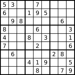
Input: board = [["8","3",".",".","7",".",".",".","."] ,["6",".",".","1","9","5",".",".","."] ,[".","9","8",".",".",".",".","6","."] ,["8",".",".",".","6",".",".",".","3"] ,["4",".",".","8",".","3",".",".","1"] ,["7",".",".",".","2",".",".",".","6"] ,[".","6",".",".",".",".","2","8","."] ,[".",".",".","4","1","9",".",".","5"] ,[".",".",".",".","8",".",".","7","9"]] Output: false Explanation: Same as Example 1, except with the 5 in the top left corner being modified to 8. Since there are two 8's in the top left 3x3 sub-box, it is invalid.
Constraints:
board.length =9=board[i].length =9=board[i][j]is a digit1-9or'.'.
※ 2.2.8.1. Constraints and Edge Cases
- only some rules given, just have to evaluate ONLY them
- no need to care about empty slots
- just need to do repetition check
※ 2.2.8.2. My Solution (Code)
My solution just runs the 3 rules separately. If there are more rules, then each rule evaluation can be function-pointered and we could just add them as we wish. The code for the frequency check is the same regardless of slice.
Also this time I didn’t have much of a problem defining the slices because I have a better intuition for why the ranges are defined like they are.
1: class Solution: 2: │ def isValidSudoku(self, board: List[List[str]]) -> bool: 3: │ │ # handle the rows: 4: │ │ for row in board: 5: │ │ │ frequency_ref = [0] * 9 # index = ord edit distance 6: │ │ │ for val in row: 7: │ │ │ │ if (val == '.'): 8: │ │ │ │ │ continue 9: │ │ │ │ idx = ord(val) - ord('1') 10: │ │ │ │ has_duplicate = frequency_ref[idx] > 0 11: │ │ │ │ if (has_duplicate): 12: │ │ │ │ │ return False 13: │ │ │ │ frequency_ref[idx] += 1 14: │ │ │ │ 15: │ │ # handle the columns: 16: │ │ for col_idx in range(0, 9): 17: │ │ │ frequency_ref = [0] * 9 # index = ord edit distance 18: │ │ │ column = (row[col_idx] for row in board) 19: │ │ │ for val in column: 20: │ │ │ │ if (val == '.'): 21: │ │ │ │ │ continue 22: │ │ │ │ idx = ord(val) - ord('1') 23: │ │ │ │ has_duplicate = frequency_ref[idx] > 0 24: │ │ │ │ if (has_duplicate): 25: │ │ │ │ │ return False 26: │ │ │ │ frequency_ref[idx] += 1 27: │ │ │ │ 28: │ │ # handle sub_boxes: 29: │ │ top_left_corners = ((row_idx_start, col_idx_start) for col_idx_start in range(0, 9, 3) for row_idx_start in range(0, 9, 3)) 30: │ │ 31: │ │ for row_start, col_start in top_left_corners: 32: │ │ │ frequency_ref = [0] * 9 # index = ord edit distance 33: │ │ │ for val in (board[row_idx][col_idx] for row_idx in range(row_start, row_start + 3) for col_idx in range(col_start, col_start + 3)): 34: │ │ │ │ if (val == '.'): 35: │ │ │ │ │ continue 36: │ │ │ │ idx = ord(val) - ord('1') 37: │ │ │ │ has_duplicate = frequency_ref[idx] > 0 38: │ │ │ │ if (has_duplicate): 39: │ │ │ │ │ return False 40: │ │ │ │ frequency_ref[idx] += 1 41: │ │ │ │ 42: │ │ return True
※ 2.2.8.2.1. Ideal Solution: Single pass simultaneous checks
1: from collections import defaultdict 2: 3: class Solution: 4: │ def isValidSudoku(self, board: List[List[str]]) -> bool: 5: │ │ cols=defaultdict(set) 6: │ │ rows=defaultdict(set) 7: │ │ squares=defaultdict(set) 8: │ │ 9: │ │ for row_idx in range(9): 10: │ │ │ for col_idx in range(9): 11: │ │ │ │ cell = board[row_idx][col_idx] 12: │ │ │ │ if (cell == '.'): 13: │ │ │ │ │ continue 14: │ │ │ │ │ 15: │ │ │ │ is_duplicate_in_rows = cell in rows[row_idx] 16: │ │ │ │ if is_duplicate_in_rows: 17: │ │ │ │ │ return False 18: │ │ │ │ rows[row_idx].add(cell) 19: │ │ │ │ 20: │ │ │ │ is_duplicate_in_columns = cell in cols[col_idx] 21: │ │ │ │ if is_duplicate_in_columns: 22: │ │ │ │ │ return False 23: │ │ │ │ cols[col_idx].add(cell) 24: │ │ │ │ 25: │ │ │ │ # squares can be mapped using their top left corner coordinate as the key: 26: │ │ │ │ top_left_corner_coord = (row_idx // 3, col_idx // 3) 27: │ │ │ │ is_duplicate_in_squares = cell in squares[top_left_corner_coord] 28: │ │ │ │ if is_duplicate_in_squares: 29: │ │ │ │ │ return False 30: │ │ │ │ squares[top_left_corner_coord].add(cell) 31: │ │ │ │ 32: │ │ return True 33:
This is superior because: Explanation:
- Each cell is checked only once: Your approach checks each cell three times (row, column, box), while the single-pass approach checks each cell once and updates all three constraints in one go.
- Immediate feedback: If a violation is found, the function returns immediately, possibly before the rest of the board is checked.
- Cache locality: Fewer passes over the data means better use of CPU cache, which can matter for larger boards.
※ 2.2.8.3. My Approach/Explanation
- for the repetition check part, it’s clear that the fixed char space for 1 to 9 digits means that we can do a very efficient way of doing fixed-array frequency checks. Just use
ord(val) - ord(-1)to get the edit distance, which becomes the index in the array. The bot praised me “Your use of ord(val) - ord(‘1’) is clever for fixed-size arrays.” - I acknowledge that my approach has 3 readings per cell and this is technically wasteful
- the rest of it is a matter of being able to define python slices correctly.
※ 2.2.8.4. My Learnings/Questions
- the edit distance as a way of judging the index within the fixed sized frequency ref-array is pretty neat!
- The single-pass approach is better for n-dimensional. In this case, it’s tolerable because the board-size is fixed.
Question: One of the better solutions online looks like this but I don’t have an under-the-hood understanding of why that is significantly faster (other than avoiding the duplicate reads for each cell)
Show/Hide Python Code1: class Solution: 2: │ def isValidSudoku(self, board: List[List[str]]) -> bool: 3: │ │ cols=defaultdict(set) 4: │ │ rows=defaultdict(set) 5: │ │ squares=defaultdict(set) 6: │ │ for r in range(9): 7: │ │ │ for c in range(9): 8: │ │ │ │ if board[r][c]==".": 9: │ │ │ │ │ continue 10: │ │ │ │ if (board[r][c] in rows[r] or board[r][c] in cols[c] or board[r][c] in squares[(r//3,c//3)]): 11: │ │ │ │ │ return False 12: │ │ │ │ cols[c].add(board[r][c]) 13: │ │ │ │ rows[r].add(board[r][c]) 14: │ │ │ │ squares[(r//3,c//3)].add(board[r][c]) 15: │ │ return True
※ 2.2.8.5. GPT Critique
Here's a detailed review and analysis of your **Valid Sudoku** solution: ## 1. **Correctness** **Your solution is correct**: - It checks all three rules: rows, columns, and 3x3 sub-boxes, for duplicate digits (ignoring '.'). - The use of a fixed-size frequency array is appropriate since only digits 1-9 are valid. - Handles all edge cases, including empty cells and full/partial boards. ## 2. **Time and Space Complexity** - **Time Complexity:** │ - For each rule (row, column, sub-box), you scan all 81 cells: 3 × 81 = **O(1)** (since the board is always 9x9), but in general, **O(n²)** for an n×n board. │ - **However, each cell is checked three times** (once per rule), which is redundant but not problematic for a fixed-size board. │ - **Space Complexity:** │ - Uses a fixed-size frequency array of length 9 for each check: **O(1)** extra space. │ ## 3. **Improvements in Code Style, Efficiency, or Clarity** - **Clarity:** │ - Code is readable and well-commented. │ - The use of `ord(val) - ord('1')` is clever and efficient for mapping digits to indices. - **Efficiency:** │ - The main inefficiency is that each cell is visited three times (once per row, column, and sub-box). │ - For a 9x9 board, this is not a real issue, but for a generalized n×n board, a single-pass approach is preferable. - **Style:** │ - You could factor out the frequency check into a helper function to reduce code repetition. │ ## 4. **Comparison to the Optimal Solution** - **Optimal Solution:** │ - The single-pass approach (as in your referenced solution) checks all three constraints in one traversal of the board, visiting each cell only once. │ - This uses three data structures (sets or arrays) to track seen digits for each row, column, and sub-box. │ **Why is it faster?** - **Fewer reads:** Each cell is processed once, not three times. - **Immediate detection:** As soon as a duplicate is found in any rule, it returns `False` without unnecessary further checks. - **Better for larger boards:** For larger or dynamic boards, this approach scales better. ## 5. **Sample Optimal Solution (Single Pass, O(1) Space and Time)** ```python from collections import defaultdict class Solution: │ def isValidSudoku(self, board: List[List[str]]) -> bool: │ │ rows = defaultdict(set) │ │ cols = defaultdict(set) │ │ boxes = defaultdict(set) │ │ for r in range(9): │ │ │ for c in range(9): │ │ │ │ val = board[r][c] │ │ │ │ if val == ".": │ │ │ │ │ continue │ │ │ │ if (val in rows[r] or │ │ │ │ │ val in cols[c] or │ │ │ │ │ val in boxes[(r // 3, c // 3)]): │ │ │ │ │ return False │ │ │ │ rows[r].add(val) │ │ │ │ cols[c].add(val) │ │ │ │ boxes[(r // 3, c // 3)].add(val) │ │ return True ``` - **Time:** O(1) for 9x9, O(n²) for n×n. - **Space:** O(1) (since max 9 elements per set). ## 6. **Pythonic Improvements** - Use of `defaultdict(set)` is idiomatic and clear. - Could use list comprehensions or generator expressions for brevity, but clarity is more important here. - You could use arrays of sets instead of `defaultdict` (since indices are always 0–8), but `defaultdict` is fine and concise. ## 7. **Your Specific Questions** > Why is the single-pass solution with sets significantly faster? **Explanation:** - **Each cell is checked only once:** │ Your approach checks each cell three times (row, column, box), while the single-pass approach checks each cell once and updates all three constraints in one go. - **Immediate feedback:** │ If a violation is found, the function returns immediately, possibly before the rest of the board is checked. - **Cache locality:** │ Fewer passes over the data means better use of CPU cache, which can matter for larger boards. │ **In summary:** The single-pass solution is more efficient in both time and space for larger or dynamic boards, and is more elegant and maintainable. ## **Summary Table** | Approach | Time per cell | # of passes | Space per constraint | Early exit? | Pythonic | |------------------|--------------|-------------|----------------------|-------------|----------| | Your solution | O(1) | 3 | O(1) | Yes | Yes | | Single-pass sets | O(1) | 1 | O(1) | Yes | Yes | ## **Conclusion** - **Your solution is correct and efficient for 9x9 boards.** - **Single-pass set-based solutions are slightly more efficient and are considered optimal for this problem.** - Your use of `ord(val) - ord('1')` is clever for fixed-size arrays. - For Pythonic style and efficiency, consider the single-pass approach. Let me know if you want to see further variants or more in-depth analysis! [1] https://leetcode.com/problems/valid-sudoku/description/
※ 2.2.9. [9] Longest Consecutive Sequence (128) med sequence accumulation
Given an unsorted array of integers nums, return the length of the
longest consecutive elements sequence.
You must write an algorithm that runs in O(n) time.
Example 1:
Input: nums = [100,4,200,1,3,2] Output: 4 Explanation: The longest consecutive elements sequence is [1, 2, 3, 4]. Therefore its length is 4.
Example 2:
Input: nums = [0,3,7,2,5,8,4,6,0,1] Output: 9
Example 3:
Input: nums = [1,0,1,2] Output: 3
Constraints:
0 <nums.length <= 10=5-10=^{=9}= <= nums[i] <= 10=9
※ 2.2.9.1. Constraints and Edge Cases
- it must run in O(n) time, so no direct sorting or anything
- however, does this mean that we can sort groups as we accumulate groups? ANS: NO such thing
- initial array is unsorted
※ 2.2.9.2. My Solution
※ 2.2.9.2.1. Initial wrong approach:
This attempted to create ranges and tried to merge intervals. However, interval merging is a difficult thing to do. In the future, if we encounter any case where we have to choose to NOT merge intervals, we should take that.
1: class Solution: 2: │ def longestConsecutive(self, nums: List[int]) -> int: 3: │ │ ranges = [] 4: │ │ for num in nums: 5: │ │ │ # any matching? 6: │ │ │ for idx, (start, end_ex) in enumerate(ranges): 7: │ │ │ │ # check if within: 8: │ │ │ │ if (num >= start and num < end_ex): 9: │ │ │ │ │ continue 10: │ │ │ │ # check if can extend the existing range: 11: │ │ │ │ if (num + 1 == start): 12: │ │ │ │ │ ranges[idx] = (num, end_ex) 13: │ │ │ │ │ continue 14: │ │ │ │ │ 15: │ │ │ │ if (num == end_ex): 16: │ │ │ │ │ ranges[idx] = (start, num + 1) 17: │ │ │ │ │ continue 18: │ │ │ │ │ 19: │ │ │ │ ranges.append((num, num + 1)) 20: │ │ │ │ 21: │ │ desc_sorted_ranges = sorted(ranges, key=lambda x: x[1] - x[0]) 22: │ │ biggest_range = desc_sorted_ranges[-1] 23: │ │ 24: │ │ return biggest_range[1] - biggest_range[0]
※ 2.2.9.2.2. Guided Improvement
The key ideas:
- We pick the start values and KEEP trying to build onto it. It’s like finding a no-op ladder when doing Return-oriented programming approach to memory attacks. ==> only try to build sequences from the start of a sequence
- We just need to do membership checks quickly and using a set is the best idea here.
- Also it helps that we don’t need to return the longest set, we just need to return its length => hints at just needing an accumulator variable that we return as the result eventually
1: class Solution: 2: │ def longestConsecutive(self, nums: List[int]) -> int: 3: │ │ allSet = set(nums) 4: │ │ curr_longest = 0 5: │ │ for num in allSet: 6: │ │ │ is_start_of_seq = (num - 1) not in allSet 7: │ │ │ if is_start_of_seq: 8: │ │ │ │ # init the length: 9: │ │ │ │ length = 1 10: │ │ │ │ current = num 11: │ │ │ │ # try climbing the "ROP NOOPladder": 12: │ │ │ │ while can_continue_climbing:= (current + 1) in allSet: 13: │ │ │ │ │ current += 1 14: │ │ │ │ │ length += 1 15: │ │ │ │ │ 16: │ │ │ │ # so now we have an interval 17: │ │ │ │ curr_longest = max(curr_longest, length) 18: │ │ │ │ 19: │ │ return curr_longest
Another improvement is to avoid the use of the current variable. We can directly use the length variable to expand the ’interval’.
1: class Solution: 2: │ def longestConsecutive(self, nums: List[int]) -> int: 3: │ │ num_set = set(nums) 4: │ │ longest = 0 5: │ │ 6: │ │ for n in num_set: 7: │ │ │ if n - 1 not in num_set: 8: │ │ │ │ length = 1 9: │ │ │ │ 10: │ │ │ │ while n + length in num_set: 11: │ │ │ │ │ length += 1 12: │ │ │ │ │ 13: │ │ │ │ longest = max(longest, length) 14: │ │ │ │ 15: │ │ return longest
※ 2.2.9.3. My Approach/Explanation
Initial failed attempt:
- My approach was to define ranges/intervals using tuples.
iterate through the nums and each time there are 3 cases:
- The num is within an existing range
- the num is to the left extending of an existing range ==> we can replace the tuple with an updated range
- the num is to the right extending of an existing range ==> we can replace the tuple with an updated range Once I’ve tried to group up all the numbers, then I just need to check if any of the existing ranges can be merged with each other to create bigger super ranges. Like a cascade of sorts. however, I don’t know how to do this cascade of sorts
Final Insight:
- it’s really just a noop sled like that: The key insight is: You only need to start climbing from the “base” of a ladder (the minimal element of a sequence)—if you start anywhere else, you’re not at the true start, and you’ll be duplicating work.
※ 2.2.9.4. My Learnings/Questions
- Problems with original solution:
- it introduces the problem of needing to merge intervals and interval-merging intervals efficiently should be seen as a hard problem
- the inner loop run makes the overall thing O(n2) which violates the requirement that we are given that it needs to be done in O(n) time.
- Interval merging efficiently should be seen as a hard problem to solve
- Key Intuition:
The key insight is: You only need to start climbing from the “base” of a ladder (the minimal element of a sequence)—if you start anywhere else, you’re not at the true start, and you’ll be duplicating work.
- We can use a set for O(1) lookups, we just need to find the start of each sequence to see if
num - 1is NOT in the set - for each “start” we can count upwards until we no longer find consecutive numbers
- We can use a set for O(1) lookups, we just need to find the start of each sequence to see if
- More intuition aspects:
When you see “longest consecutive sequence” and an O(n) requirement, think:
- Can I use a set for O(1) lookups?
- Can I only start counting at the minimal element of a sequence? Avoid interval merging unless the problem is specifically about merging sorted intervals.
Extensions, more on interval merging:
Show/Hide Md CodeThe **most efficient and standard way to merge intervals** is as follows: ### **1. Sort the intervals by their start time** Sorting ensures that any overlapping intervals are adjacent, so you only need to compare each interval to the last merged one[1][2][3][5][6][7][9]. ### **2. Iterate and merge** - Initialize a result list with the first interval. - For each subsequent interval: │ - If it overlaps with the last interval in the result (i.e., its start is less than or equal to the end of the last merged interval), merge them by updating the end of the last interval to the maximum of both ends. │ - If it does not overlap, simply append it to the result list. │ ### **3. Time Complexity** - **Sorting:** O(n log n) - **Merging:** O(n) - **Total:** O(n log n) (dominated by the sorting step)[3][5][6][7]. #### **Python Example** ```python def merge(intervals): │ if not intervals: │ │ return [] │ # Step 1: Sort intervals by start time │ intervals.sort(key=lambda x: x[0]) │ merged = [intervals[0]] │ # Step 2: Iterate and merge │ for current in intervals[1:]: │ │ last = merged[-1] │ │ if current[0] <= last[1]: │ │ │ # Overlap: merge │ │ │ last[1] = max(last[1], current[1]) │ │ else: │ │ │ # No overlap: add new interval │ │ │ merged.append(current) │ return merged ``` ### **Why Not O(n)?** - The need to sort the intervals by start time is fundamental for efficient merging; without sorting, you’d need to check all pairs, which is O(n²)[3][5]. - There are advanced data structures (like interval trees or balanced BSTs) that can support dynamic merging in streaming scenarios, but for the classic merge-intervals problem, **O(n log n)** via sorting is optimal and standard[10]. ### **Summary Table** | Approach | Time Complexity | When to Use | |--------------------|----------------|----------------------------------------------| | Sort + Merge (std) | O(n log n) | Most general and efficient for static input | | Naive (nested) | O(n²) | Only for very small input or educational use | | Interval Tree | O(n log n) | For dynamic/streaming intervals | **In short:** **Sort by start time, then merge adjacent intervals in a single pass. This is the most efficient and standard approach for merging intervals.**[1][2][3][5][6] If you need to handle intervals in a streaming fashion (i.e., intervals arrive one at a time), an interval tree or balanced BST can be used for efficient dynamic merging, but that’s a more advanced scenario[10]. [1] https://algocademy.com/blog/merge-intervals-a-comprehensive-guide-to-solving-this-classic-algorithm-problem/ [2] https://www.architectalgos.com/mastering-merge-interval-patterns-a-guide-to-solving-interval-based-problems-1a14ef065876 [3] https://www.geeksforgeeks.org/dsa/merging-intervals/ [4] https://leetcode.com/problems/merge-intervals/ [5] https://www.educative.io/interview-prep/coding/solution-merge-intervals [6] https://algocademy.com/blog/mastering-merge-interval-problems-essential-techniques-for-coding-interviews/ [7] https://docs.vultr.com/problem-set/merge-intervals [8] https://www.w3resource.com/data-structures-and-algorithms/array/dsa-merge-intervals.php [9] https://blog.seancoughlin.me/mastering-the-merging-of-overlapping-intervals-in-python [10] https://stackoverflow.com/questions/4748184/how-to-efficiently-merge-int-ranges-in-a-stream
※ 2.2.9.5. GPT Guidance for Intuition
Here's a thorough evaluation of your **Longest Consecutive Sequence** solution and the concepts behind the optimal approach: ## 1. **Correctness of Your Solution** Your approach tries to build and extend ranges (intervals) as you iterate through `nums`, but: - **It is not correct** for several reasons: │ - You may create overlapping intervals that are never merged (e.g., `[1]` and `` should become `[1]`). │ - You may miss merging intervals that are adjacent after an extension. │ - The inner loop over all current ranges for every number makes it **O(n²)**, not O(n). │ - The logic for updating and merging intervals is incomplete and does not handle all cases. │ **Example of failure:** Given `[1][1]`, your code could create intervals like `[1]`, ``, `[1]` but never merges them, so it won't find the correct answer. ## 2. **Time and Space Complexity** - **Time Complexity:** │ - Your code is **O(n²)** in the worst case, since for each number you may iterate over all current ranges. - **Space Complexity:** │ - Up to O(n) for the `ranges` list. │ ## 3. **Improvements in Code Style, Efficiency, or Clarity** - **Clarity:** │ - The interval approach is not wrong in spirit, but merging intervals efficiently is hard without sorting or auxiliary structures. - **Efficiency:** │ - The O(n²) approach is not acceptable for large inputs. - **Code Style:** │ - Variable names are clear, but the logic is convoluted due to the merging issue. │ ## 4. **Comparison to the Optimal Solution** ### **Optimal Solution Intuition** - **Key Insight:** │ - If you use a set for O(1) lookups, you can find the start of each sequence by checking if `num - 1` is not in the set. │ - For every such "start", you can count upwards until you no longer find consecutive numbers. │ ### **Optimal Solution (O(n) time, O(n) space)** ```python class Solution: │ def longestConsecutive(self, nums: List[int]) -> int: │ │ num_set = set(nums) │ │ longest = 0 │ │ │ │ for num in num_set: │ │ │ # Only try to build sequences from the start of a sequence │ │ │ if num - 1 not in num_set: │ │ │ │ current = num │ │ │ │ length = 1 │ │ │ │ while current + 1 in num_set: │ │ │ │ │ current += 1 │ │ │ │ │ length += 1 │ │ │ │ longest = max(longest, length) │ │ │ │ │ │ return longest ``` - **Why is this O(n)?** │ - Each number is only visited once as the start of a sequence. │ - The inner `while` only runs across the length of each sequence, and all numbers are only processed once in total. │ ## 5. **Pythonic Improvements** - Use a set for O(1) lookups. - Avoid unnecessary sorting or interval merging. - Use clear variable names (`longest`, `current`, `length`). ## 6. **Your Specific Questions** ### **Q1: What makes this different from typical greedy solutions? How can I pattern-recognise better?** - **Difference:** │ - The greedy part is recognizing that you only need to start counting from the smallest number in a sequence (i.e., when `num - 1` is not in the set). │ - The pattern to recognize: │ - When asked for "longest consecutive sequence" in O(n), think about using a set for fast membership and only starting new sequences at the minimal elements. │ ### **Q2: What's wrong with my solution?** - **Main Issues:** │ - Inefficient (O(n²)) due to nested loops. │ - Fails to merge/extend intervals correctly. │ - Not scalable for large inputs. │ ## 7. **Summary Table** | Approach | Time Complexity | Space Complexity | Handles Merging? | O(n)? | Pythonic? | |-------------------|----------------|------------------|------------------|-------|-----------| | Your intervals | O(n²) | O(n) | ❌ | ❌ | Somewhat | | Set-based optimal | O(n) | O(n) | ✅ | ✅ | ✅ | ## **Conclusion** - Your approach is creative but not efficient or correct for all cases. - The optimal solution uses a set and only starts counting at sequence starts, resulting in O(n) time and O(n) space. - Pattern recognition: When O(n) is required for "consecutive" problems, consider using a set for O(1) lookups and avoid redundant work. **Let me know if you want to see more alternative approaches or have other questions!** [1] https://leetcode.com/problems/longest-consecutive-sequence/description/
※ 2.2.10. [Depth-1] Subarray Sum Equals K (560) prefix_sum
Given an array of integers nums and an integer k, return the total
number of subarrays whose sum equals to k.
A subarray is a contiguous non-empty sequence of elements within an array.
Example 1:
Input: nums = [1,1,1], k = 2 Output: 2
Example 2:
Input: nums = [1,2,3], k = 3 Output: 2
Constraints:
1 <nums.length <= 2 * 10=4-1000 <nums[i] <= 1000=-10=^{=7}= <= k <= 10=7
※ 2.2.10.1. Constraints and Edge Cases
- there’s negative numbers so this means that the same prefix sum value may appear more than once
※ 2.2.10.2. My Solution (Code)
※ 2.2.10.2.1. v0: flawed, almost, double counting
1: from collections import defaultdict 2: 3: class Solution: 4: │ def subarraySum(self, nums: List[int], k: int) -> int: 5: │ │ n = len(nums) 6: │ │ prefix_sums = [0] * (n + 1) 7: │ │ # because we have negative numbers, we can expect to have multiple values of the same prefix sum, at different indices 8: │ │ # prefix sums to count 9: │ │ ref = defaultdict(int) 10: │ │ ref[0] = 1 11: │ │ 12: │ │ # creates the prefix sums 13: │ │ for i in range(1, n + 1): 14: │ │ │ prefix_sum = nums[i - 1] + prefix_sums[i - 1] 15: │ │ │ prefix_sums[i] = prefix_sum 16: │ │ │ ref[prefix_sum] += 1 17: │ │ │ 18: │ │ counts = 0 19: │ │ 20: │ │ for i in range(1, n + 1): 21: │ │ │ curr = prefix_sums[i] 22: │ │ │ complement = curr - k 23: │ │ │ counts += ref[complement] 24: │ │ │ 25: │ │ return counts
this double counts:
- my ref is just a trivial count. so, this means that I will be wrongly accepting values > i in that for loop and that would get counted again. that’s how the double counting gets introduced.
a quick fix would be to store indices but that’s awfully slow (thought it will pass all testcases)
Show/Hide Python Code1: from collections import defaultdict 2: 3: class Solution: 4: │ def subarraySum(self, nums: List[int], k: int) -> int: 5: │ │ n = len(nums) 6: │ │ prefix_sums = [0] * (n + 1) 7: │ │ # because we have negative numbers, we can expect to have multiple values of the same prefix sum, at different indices 8: │ │ # prefix sums to count 9: │ │ ref = defaultdict(list) 10: │ │ ref[0].append(0) 11: │ │ 12: │ │ # creates the prefix sums 13: │ │ for i in range(1, n + 1): 14: │ │ │ prefix_sum = nums[i - 1] + prefix_sums[i - 1] 15: │ │ │ prefix_sums[i] = prefix_sum 16: │ │ │ ref[prefix_sum].append(i) 17: │ │ │ 18: │ │ counts = 0 19: │ │ 20: │ │ for i in range(1, n + 1): 21: │ │ │ curr = prefix_sums[i] 22: │ │ │ complement = curr - k 23: │ │ │ counts += len([idx for idx in ref[complement] if idx < i]) 24: │ │ │ 25: │ │ │ 26: │ │ return counts
※ 2.2.10.2.2. v1: optimal, single pass solution.
1: from collections import defaultdict 2: 3: class Solution: 4: │ def subarraySum(self, nums: List[int], k: int) -> int: 5: │ │ n = len(nums) 6: │ │ # number of already seen prefix counts -- remember it's a historical 7: │ │ prefix_count = defaultdict(int) 8: │ │ prefix_count[0] = 1 # the first idx is 0 trivially and we have seen it once 9: │ │ curr_sum = 0 10: │ │ 11: │ │ res = 0 12: │ │ 13: │ │ for num in nums: 14: │ │ │ curr_sum += num 15: │ │ │ if (complement:=curr_sum - k) in prefix_count: 16: │ │ │ │ res += prefix_count[complement] 17: │ │ │ prefix_count[curr_sum] += 1 18: │ │ │ 19: │ │ return res
This in a way is a compressed dp solution. Better to describe this canonically as prefix sum / range sum solution.
※ 2.2.10.3. My Approach/Explanation
- this is a subarray sum. Classical question for prefix-sum approaches.
※ 2.2.10.4. My Learnings/Questions
- prefix sum approaches to solving range sum type questions.
- careful:
- single pass, order of filling the prefix sum table matters
- remember the trivial helper values (e.g.
prefix_count[0] = 1)
- sliding window would ONLY have worked here if we had NO non-negative values
- the v1 solution can be interpreted as a DP solution as well:
- Dynamic Programming?
- Yes — we store the counts of prefix sums (that’s memoization of subproblems).
- Optimal substructure: The count of valid subarrays ending at index i depends on best solutions to subproblems ending earlier (j < i).
- Overlapping subproblems: many subarrays share the same prefix sums, so we reuse them via hashmap.
- So your v1 approach is really prefix-sum DP disguised as hashing.
- Dynamic Programming?
※ 2.2.11. [exposure-1] Sort Vowels in a String (2785)
Given a 0-indexed string s, permute s to get a new string t
such that:
- All consonants remain in their original places. More formally, if
there is an index
iwith0 <i < s.length= such thats[i]is a consonant, thent[i] = s[i]. - The vowels must be sorted in the nondecreasing order of their
ASCII values. More formally, for pairs of indices
i,jwith0 <i < j < s.length= such thats[i]ands[j]are vowels, thent[i]must not have a higher ASCII value thant[j].
Return the resulting string.
The vowels are 'a', 'e', 'i', 'o', and 'u', and they can
appear in lowercase or uppercase. Consonants comprise all letters that
are not vowels.
Example 1:
Input: s = "lEetcOde" Output: "lEOtcede" Explanation: 'E', 'O', and 'e' are the vowels in s; 'l', 't', 'c', and 'd' are all consonants. The vowels are sorted according to their ASCII values, and the consonants remain in the same places.
Example 2:
Input: s = "lYmpH" Output: "lYmpH" Explanation: There are no vowels in s (all characters in s are consonants), so we return "lYmpH".
Constraints:
1 <s.length <= 10=5sconsists only of letters of the English alphabet in uppercase and lowercase.
※ 2.2.11.1. Constraints and Edge Cases
Nothing fancy, the inputs imply that it has to be in linear time.
※ 2.2.11.2. My Solution (Code)
※ 2.2.11.2.1. v0 my solution, correct, decent
1: from collections import Counter 2: class Solution: 3: │ def sortVowels(self, s: str) -> str: 4: │ │ counts = Counter(s) 5: │ │ vowels = list("aeiouAEIOU") 6: │ │ is_vowel = lambda x: x in vowels 7: │ │ for char in list(counts.keys()): 8: │ │ │ if not is_vowel(char): 9: │ │ │ │ del counts[char] 10: │ │ supply = [] 11: │ │ for char, freq in sorted(counts.items()): 12: │ │ │ supply.extend([char] * freq) 13: │ │ gen_vowels = iter(supply) 14: │ │ 15: │ │ res = [] 16: │ │ for char in s: 17: │ │ │ if not is_vowel(char): 18: │ │ │ │ res.append(char) 19: │ │ │ │ continue 20: │ │ │ │ 21: │ │ │ res.append(next(gen_vowels)) 22: │ │ │ 23: │ │ return "".join(res)
- Improvements
- Efficiency & Clarity
- Counting and filtering is unnecessary—extract vowels during a single pass, sort, and then use them.
- Membership check via char in vowels is O(1) with a set, whereas with a list, it’s O(1) amortized for 10 elements, but using a set is idiomatic and very clear.
- The generator and extend/Counter logic is correct but could be streamlined for readability.
- Pythonic Style
- Consider using a set for vowels:
vowels = set("aeiouAEIOU")membership check is faster with this. - Use a descriptive variable name for the vowel supply (e.g., sortedvowels).
- Lambda for
is_vowelcould be replaced by an inline check for clarity or a top-level function.
- Consider using a set for vowels:
- Efficiency & Clarity
So, cleaner:
1: class Solution: 2: │ def sortVowels(self, s: str) -> str: 3: │ │ vowels = set("aeiouAEIOU") # set allows for fast membership checks 4: │ │ sorted_vowels = sorted([ch for ch in s if ch in vowels]) 5: │ │ res = [] 6: │ │ idx = 0 7: │ │ for ch in s: 8: │ │ │ if ch in vowels: 9: │ │ │ │ res.append(sorted_vowels[idx]) 10: │ │ │ │ idx += 1 11: │ │ │ else: 12: │ │ │ │ res.append(ch) 13: │ │ return "".join(res)
※ 2.2.11.3. My Approach/Explanation
My solution just uses python language features (counters, enumeration, generators) and makes the performance alright, nothing fancy here.
※ 2.2.11.4. My Learnings/Questions
- first time I used generators like that.
※ 2.2.11.5. Prompt for GPT Evaluation
Please do the following:
- Evaluate the correctness of my solution. Are there any logical or edge case errors?
- Analyze the time and space complexity of my code.
- Suggest improvements in code style, efficiency, or clarity.
- Compare my approach to the optimal solution (if different).
- Provide a sample optimal solution (if mine is not optimal).
- Point out any Pythonic (or language-specific) improvements.
Are there any completely different approaches to this problem?
- e.g something that uses a completely different data structure
If so, then help me gain the intuition for it and show the code clearly
- Answer my specific questions (if any are listed above).
※ 2.2.11.6. Prompt for GPT Evaluation (with Greedy)
Please do the following:
- Evaluate the correctness of my solution. Are there any logical or edge case errors?
- Analyze the time and space complexity of my code.
- Suggest improvements in code style, efficiency, or clarity.
- Compare my approach to the optimal solution (if different).
- Provide a sample optimal solution (if mine is not optimal).
- Point out any Pythonic (or language-specific) improvements.
Are there any completely different approaches to this problem?
- e.g something that uses a completely different data structure
If so, then help me gain the intuition for it and show the code clearly
- Answer my specific questions (if any are listed above).
ALso help me evaluate this in the context of greedy algorithms, ensuring that a good framework of presenting this problem into a greedy algo is given / understood.
※ 2.2.11.7. Prompt for GPT Evaluation (with DP)
Please do the following:
- Evaluate the correctness of my solution. Are there any logical or edge case errors?
- Analyze the time and space complexity of my code.
- Suggest improvements in code style, efficiency, or clarity.
- Compare my approach to the optimal solution (if different).
- Provide a sample optimal solution (if mine is not optimal).
- Point out any Pythonic (or language-specific) improvements.
Are there any completely different approaches to this problem?
- e.g something that uses a completely different data structure
If so, then help me gain the intuition for it and show the code clearly
- Answer my specific questions (if any are listed above).
ALso help me evaluate this in the context of greedy algorithms, ensuring that a good framework of presenting this problem into a greedy algo is given / understood.
Additionally, use my notes for Dynamic Programming and use the recipes that are here.
Recipe to define a solution via DP
[Generate Naive Recursive Algo]
Characterise the structure of an optimal solution \(\implies\) what are the subproblems? \(\implies\) are they independent subproblems? \(\implies\) how many subproblems will there be?
- Recursively define the value of an optimal solution \(\implies\) does this have the overlapping sub-problems property? \(\implies\) what’s the cost of making a choice? \(\implies\) how many ways can I make that choice?
- Compute value of an optimal solution
- Construct optimal solution from computed information Defining things
- Optimal Substructure:
A problem exhibits “optimal substructure” if an optimal solution to the problem contains within it optimal solutions to subproblems.
Elements of Dynamic Programming: Key Indicators of Applicability [1] Optimal Sub-Structure Defining “Optimal Substructure” A problem exhibits optimal substructure if an optimal solution to the problem contains within it optimal solutions to sub-problems.
- typically a signal that DP (or Greedy Approaches) will apply here.
- this is something to discover about the problem domain Common Pattern when Discovering Optimal Substructure
solution involves making a choice e.g. choosing an initial cut in the rod or choosing what k should be for splitting the matrix chain up
\(\implies\) making the choice also determines the number of sub-problems that the problem is reduced to
- Assume that the optimal choice can be determined, ignore how first.
- Given the optimal choice, determine what the sub-problems looks like \(\implies\) i.e. characterise the space of the subproblems
- keep the space as simple as possible then expand
typically the substructures vary across problem domains in 2 ways:
[number of subproblems]
how many sub-problems does an optimal solution to the original problem use?
- rod cutting:
# of subproblems = 1(of size n-i) where i is the chosen first cut lengthmatrix split:
# of subproblems = 2(left split and right split)[number of subproblem choices]
how many choices are there when determining which subproblems(s) to use in an optimal solution. i.e. now that we know what to choose, how many ways are there to make that choice?
- rod cutting: # of choices for i = length of first cut,
nchoices- matrix split: # of choices for where to split (idx k) =
j - iNaturally, this is how we analyse the runtime:
# of subproblems * # of choices @ each sub-problem- Reason to yourself if and how solving the subproblems that are used in an optimal solution means that the subproblem-solutions are also optimal. This is typically done via the
cut-and-paste argument.Caveat: Subproblems must be
independent
- “independent subproblems”
- solution to one subproblem doesn’t affect the solution to another subproblem for the same problem
example: Unweighted Shortest Path (independent subproblems) vs Unweighted Longest Simple Path (dependent subproblems)
Consider graph \(G = (V,E)\) with vertices \(u,v \notin V\)
- Unweighted shortest path: we want to find path \(u\overset{p}{\leadsto}v\) then we can break it down into subpaths \(u\overset{p1}{\leadsto}w\overset{p2}{\leadsto}v\) (optimal substructure). If path, p, is optimal from \(u\leadsto{v}\) then p1 must be shortest path from \(u\leadsto{w}\) and likewise p2 must be shortest path from \(w\leadsto{v}\) (cut-and-paste argument) Here, we know that the subproblems are independent.
- Unweighted Longest Simple Path: the subproblems can have paths that overlap (not subproblem overlap), hence it’s not independent because the vertices that appear can appear in the solution to the second subproblem
Terminology: Optimal substruture vs optimal solution optimal substructure is a property that enables efficient computation of the optimal value, while the solution is the specific configuration that yields that optimal value
You’re right that in dynamic programming algorithms for optimization problems, the goal is usually to find an optimal solution rather than the unique optimal solution. Here’s how the optimal substructure and the actual solution differ:
### Optimal Substructure
The optimal substructure refers to the property that the optimal solution to a problem can be constructed from the optimal solutions to its subproblems. This means that if we know the optimal solutions to the subproblems, we can efficiently determine the optimal solution to the overall problem.
For example, in the rod cutting problem, if we know the maximum revenue for rods of length 1 to n-1, we can efficiently determine the maximum revenue for a rod of length n by considering cutting the rod at each possible length and taking the maximum revenue.
### The Solution
The actual solution, on the other hand, refers to the specific configuration or set of choices that yields the optimal value. In the rod cutting problem, the solution would be the specific way to cut the rod that results in the maximum revenue.
The key difference is that the optimal substructure allows us to efficiently compute the optimal value, but it doesn’t necessarily specify the exact solution. There may be multiple solutions that yield the same optimal value.
For example, in the rod cutting problem, there may be multiple ways to cut the rod that result in the same maximum revenue. The optimal substructure allows us to efficiently compute the maximum revenue, but it doesn’t specify which particular cutting configuration to choose.
So in summary, the optimal substructure is a property that enables efficient computation of the optimal value, while the solution is the specific configuration that yields that optimal value. Dynamic programming algorithms leverage the optimal substructure to efficiently compute the optimal value, but the actual solution may not be uniquely determined.
Citations: [1] https://library.fiveable.me/key-terms/programming-for-mathematical-applications/optimal-substructure [2] https://afteracademy.com/blog/optimal-substructure-and-overlapping-subproblems/ [3] https://www.geeksforgeeks.org/optimal-substructure-property-in-dynamic-programming-dp-2/ [4] https://labuladong.gitbook.io/algo-en/i.-dynamic-programming/optimalsubstructure [5] https://stackoverflow.com/questions/33563230/optimal-substructure-in-dynamic-programing [6] https://en.wikipedia.org/wiki/Optimal_substructure [7] https://www.cs.cmu.edu/~15451-f22/lectures/lec09-dp1.pdf [8] https://www.javatpoint.com/optimal-substructure-property
[2] Overlapping Sub-Problems
- DP should be disambiguated from Divide & Conquer:
- for Divide&Conquer, choosing a division point generates brand new problems that likely don’t overlap
- for DP, the space of sub-problems is small and hence if done purely recursively, the same operations get computed multiple times
[Practical point] Reconstructing an optimal solution Since one way to look at DP is table-filling, we typically have:
- table of costs
- table of optimal choices
the table of optimal choices can be built from the table of costs, but we want to avoid recalculating the optimal choices
Memoisation as an alternative
- the textbook used sees this as an alternative and memoised tables as the aux DS for recursive, top-down approaches
- memoisation also exploits the observation that the space of the subproblems is small and hence overlapping
Common Misconceptions Here are some common misconception, based on what perplexity says
Based on the search results, here are some of the common misconceptions that learners have about dynamic programming:
## 1. Misconceptions about the Definition and Purpose of Dynamic Programming
- Thinking that recursion and dynamic programming are explicitly different concepts[3].
- Believing that dynamic programming is exclusively used to solve optimization problems[3].
## 2. Misconceptions about the Optimal Substructure Property
- Assuming that the optimal solution to a problem can be constructed from any combination of optimal solutions to its subproblems, rather than specific optimal solutions to the right subproblems[1][2].
- Thinking that the optimal solution to a problem can be constructed from optimal solutions to unrelated subproblems[4].
## 3. Misconceptions about Memoization and Tabulation
- Failing to recognize that memoization (top-down) and tabulation (bottom-up) are two different implementation strategies for dynamic programming[1][2].
- Believing that memoization always involves recursion and tabulation always involves iteration[1][2].
## 4. Misconceptions about the Filling Order of the DP Table
- Assuming that the DP table must always be filled in a specific order (e.g., always from small to big cases), without understanding that the order depends on the problem’s dependencies and constraints[1][2][4].
## 5. Misconceptions about the Relationship between Subproblems
- Thinking that the solutions to all subproblems are needed to solve the original problem, rather than understanding that only specific optimal solutions to the right subproblems are needed[1][2].
## 6. Misconceptions about the Efficiency of Dynamic Programming
- Believing that dynamic programming always leads to polynomial-time algorithms, without understanding that it can sometimes only slightly improve the exponential-time complexity[4].
Understanding and addressing these common misconceptions can help learners develop a more accurate and comprehensive understanding of dynamic programming and its applications.
Citations: [1] https://dl.acm.org/doi/10.1145/3159450.3159528 [2] https://dl.acm.org/doi/abs/10.1145/3159450.3159528 [3] https://ics.uci.edu/~mikes/papers/Student_Misconceptions_Dynamic_Programming.pdf [4] https://www.cs.cmu.edu/~15451-f22/lectures/lec09-dp1.pdf [5] https://www.reddit.com/r/compsci/comments/er05hn/help_me_wrap_my_head_around_dynamic_programming/ [6] https://yourbasic.org/algorithms/dynamic-programming-explained/ [7] https://stackoverflow.com/questions/33563230/optimal-substructure-in-dynamic-programing [8] https://lec.inf.ethz.ch/DA/2020/slides/daLecture13.en.pdf
Greedy Algos vs DP When comparing greedy strategies and dynamic programming (DP), it’s essential to understand how they differ in methodology, application, and the nature of the problems they solve. Both approaches involve identifying optimal substructures, but they apply this concept in distinct ways. Here’s a detailed disambiguation based on the search results:
### 1. Definition and Approach
- Greedy Strategy:
- A greedy algorithm makes the most optimal choice at each step with the hope that these local optimum choices will lead to a global optimum solution. It does not consider the overall impact of the current choice on future decisions.
- Greedy algorithms are typically simpler and faster to implement, as they do not require storing results of subproblems. However, they do not guarantee an optimal solution for all problems.
- Dynamic Programming:
- Dynamic programming is a technique used to solve complex problems by breaking them down into simpler subproblems. It is based on the principles of optimal substructure and overlapping subproblems.
- DP guarantees an optimal solution by considering all possible cases and storing the results of subproblems to avoid redundant computations. This can lead to higher time and space complexity compared to greedy algorithms.
### 2. Optimal Substructure
- Greedy Algorithms:
- Greedy algorithms rely on the greedy choice property, which means that a locally optimal choice leads to a globally optimal solution. However, this property does not hold for all problems, which is why greedy algorithms may fail to find the optimal solution in some cases.
- Dynamic Programming:
- Dynamic programming explicitly uses the optimal substructure property, where an optimal solution to a problem can be constructed from optimal solutions of its subproblems. DP ensures that all relevant subproblems are considered, leading to a guaranteed optimal solution.
### 3. Subproblem Reuse
- Greedy Strategy:
- Greedy algorithms typically do not reuse solutions to subproblems. Each decision is made independently based on the current state without revisiting previous choices.
- Dynamic Programming:
- DP explicitly solves and caches solutions to overlapping subproblems. This reuse of subproblem solutions is a key feature of dynamic programming, allowing for efficient computation.
### 4. Complexity and Efficiency
- Greedy Algorithms:
- Greedy algorithms are generally more efficient in terms of time complexity due to their straightforward approach. They often run in linear or logarithmic time, depending on the problem.
- They are suitable for problems where local optimization leads to global optimization, such as in minimum spanning trees or certain shortest path problems.
- Dynamic Programming:
- DP can be less efficient than greedy algorithms in terms of time complexity, especially if every possible solution is computed. However, proper use of memoization can mitigate this.
- DP is applicable to problems with overlapping subproblems and optimal substructure, such as the Fibonacci sequence, longest common subsequence, or knapsack problems.
### 5. Examples
- Greedy Algorithms:
- Common examples include:
- Fractional Knapsack Problem: Where you can take fractions of items.
- Minimum Spanning Tree: Algorithms like Prim’s and Kruskal’s.
- Huffman Coding: For optimal prefix codes.
- Dynamic Programming:
- Common examples include:
- 0/1 Knapsack Problem: Where you cannot take fractions of items.
- Longest Common Subsequence: Finding the longest subsequence present in both sequences.
- Matrix Chain Multiplication: Finding the most efficient way to multiply a given sequence of matrices.
### Conclusion
In summary, while both greedy strategies and dynamic programming involve the concept of optimal substructure, they differ significantly in their approach to problem-solving. Greedy algorithms make decisions based on local optimality without revisiting previous choices, whereas dynamic programming systematically considers all possible subproblems and their solutions to ensure a globally optimal result. Understanding these differences allows for better problem-solving strategies and the appropriate application of each method based on the problem’s characteristics.
Citations: [1] https://www.boardinfinity.com/blog/greedy-vs-dp/ [2] https://www.shiksha.com/online-courses/articles/difference-between-greedy-and-dynamic-programming-blogId-158053 [3] https://www.interviewbit.com/blog/difference-between-greedy-and-dynamic-programming/ [4] https://stackoverflow.com/questions/16690249/what-is-the-difference-between-dynamic-programming-and-greedy-approach [5] https://www.geeksforgeeks.org/greedy-approach-vs-dynamic-programming/ [6] https://byjus.com/gate/difference-between-greedy-approach-and-dynamic-programming/ [7] https://www.cs.cmu.edu/~15451-f22/lectures/lec09-dp1.pdf [8] https://ics.uci.edu/~mikes/papers/Student_Misconceptions_Dynamic_Programming.pdf
General Takeaways Bottom-up vs Top-Down
- we can use a subproblem graph to show the relationship with the subproblems ==> diff b/w bottom up and top-down is how these deps are handled (recursive-called or soundly iterated with a proper direction)
- aysymptotic runtime is pretty similar since both solve similar \(\Omega(n^{2})\)
- Bottom up:
- basically considers order at which the subproblems are solved
- because of the ordered way of solving the smaller sub-problems first, there’s no need for recursive calls and code can be iterative entirely
- so no overhead from function calls
- no chance of stack overflow
- benefits from data-locality
- a way to see the vertices of the subproblem graph such that the subproblems y-adjacent to a given subproblem x is solved before subproblem x is solved
※ 2.2.11.8. [Optional] Additional Context
<e.g., “I struggled with X”, “I want to know about alternative algorithms”, etc.>
※ 2.3. Two Pointers
| Headline | Time | ||
|---|---|---|---|
| Total time | 4:11 | ||
| Two Pointers | 4:11 | ||
| [10] Valid Palindrome (125) | 0:34 | ||
| [11] Two Sum II - Input Array Is… | 0:19 | ||
| [12] 3 Sum (15) | 1:39 | ||
| [13] Container with the Most Water (11) | 0:54 | ||
| [14] Trapping Rainwater (42) | 0:45 |
※ 2.3.1. [10] Valid Palindrome (125)
A phrase is a palindrome if, after converting all uppercase letters into lowercase letters and removing all non-alphanumeric characters, it reads the same forward and backward. Alphanumeric characters include letters and numbers.
Given a string s, return true if it is a palindrome, or false
otherwise.
Example 1:
Input: s = "A man, a plan, a canal: Panama" Output: true Explanation: "amanaplanacanalpanama" is a palindrome.
Example 2:
Input: s = "race a car" Output: false Explanation: "raceacar" is not a palindrome.
Example 3:
Input: s = " " Output: true Explanation: s is an empty string "" after removing non-alphanumeric characters. Since an empty string reads the same forward and backward, it is a palindrome.
Constraints:
1 <s.length <= 2 * 10=5sconsists only of printable ASCII characters.
※ 2.3.1.1. Constraints and Edge Cases
- Case insensitive
- we need to ignore non alnum:
alnum check can be done in python using
"mystring".isalnum()or'a'.isalnum()and that’s really convenient. - main edge case that slowed me down: “empty string” conditions. In the case of the moving pointer, it means that the left and right pointers are at the end and beginning of the list respectively.
※ 2.3.1.2. My Solution (Code)
※ 2.3.1.2.1. Initial solution
The space use is great but the runtime speed is not good with respect to the population. It’s in-place so space is O(1) and the speed is O(n) because we need each character to at most visit once.
1: class Solution: 2: │ def isPalindrome(self, s: str) -> bool: 3: │ │ left, right = 0, len(s) - 1 4: │ │ while notOverrun:=left < right: 5: │ │ │ # keep moving left if not alnum 6: │ │ │ while canBeIgnored:= not s[left].isalnum() and left < len(s) -1: 7: │ │ │ │ left += 1 8: │ │ │ # keep moving right if not alnum 9: │ │ │ while (canBeIgnored:= not s[right].isalnum() and right > 0): 10: │ │ │ │ right -= 1 11: │ │ │ │ 12: │ │ │ # edge case: if left and right are both at the end of the array: 13: │ │ │ has_no_alnum = left == len(s) - 1 and right == 0 14: │ │ │ if has_no_alnum: 15: │ │ │ │ return True 16: │ │ │ │ 17: │ │ │ # else, there's matching that can be done: 18: │ │ │ isNotMatching = s[left].lower() != s[right].lower() 19: │ │ │ if(isNotMatching): 20: │ │ │ │ return False 21: │ │ │ │ 22: │ │ │ left += 1 23: │ │ │ right -= 1 24: │ │ │ 25: │ │ return True
※ 2.3.1.2.2. Optimal Solution (Standard 2 pointer)
The logic here is just simpler from what I had in mind.
What this seems to do is to join together the canShiftPointerFurther and does both the relative check (whether left and right pointers have overrun) as well as the alnum check.
1: class Solution: 2: │ def isPalindrome(self, s: str) -> bool: 3: │ │ left, right = 0, len(s) - 1 4: │ │ while left < right: 5: │ │ │ while left < right and not s[left].isalnum(): 6: │ │ │ │ left += 1 7: │ │ │ while left < right and not s[right].isalnum(): 8: │ │ │ │ right -= 1 9: │ │ │ if s[left].lower() != s[right].lower(): 10: │ │ │ │ return False 11: │ │ │ left += 1 12: │ │ │ right -= 1 13: │ │ return True
※ 2.3.1.2.3. Slow, Preprocessed Version (O(n) time O(n) space)
This is the most succinct.
In this case, the filtering is the pre-processing.
1: class Solution: 2: │ def isPalindrome(self, s: str) -> bool: 3: │ │ filtered = [c.lower() for c in s if c.isalnum()] 4: │ │ return filtered == filtered[::-1]
※ 2.3.1.3. My Approach/Explanation
- Ignoring other pythonic stdlib solutions, or using any other aux data structure here because the input constraint can be big.
- It’s a converging 2 pointer solution, we just do until they overrun. At each iteration, either pointer may shift more than once – kinda greedy.
※ 2.3.1.4. My Learnings/Questions
※ 2.3.2. [11] Two Sum II - Input Array Is Sorted (167)
Given a 1-indexed array of integers numbers that is already sorted
in non-decreasing order, find two numbers such that they add up to a
specific target number. Let these two numbers be
numbers[index=_{=1}=]= and numbers[index=_{=2}=]= where
1 < index=1= < index=2= <= numbers.length=.
Return the indices of the two numbers, index=_{=1} and
index=_{=2}/, added by one as an integer array/
[index=_{=1}=, index=2=]= of length 2.
The tests are generated such that there is exactly one solution. You may not use the same element twice.
Your solution must use only constant extra space.
Example 1:
Input: numbers = [2,7,11,15], target = 9 Output: [1,2] Explanation: The sum of 2 and 7 is 9. Therefore, index1 = 1, index2 = 2. We return [1, 2].
Example 2:
Input: numbers = [2,3,4], target = 6 Output: [1,3] Explanation: The sum of 2 and 4 is 6. Therefore index1 = 1, index2 = 3. We return [1, 3].
Example 3:
Input: numbers = [-1,0], target = -1 Output: [1,2] Explanation: The sum of -1 and 0 is -1. Therefore index1 = 1, index2 = 2. We return [1, 2].
Constraints:
2 <numbers.length <= 3 * 10=4-1000 <numbers[i] <= 1000=numbersis sorted in non-decreasing order.-1000 <target <= 1000=- The tests are generated such that there is exactly one solution.
※ 2.3.2.1. Constraints and Edge Cases
- there’s definitely a solution, so no fallthrough necessary
- It’s 1-indexed. This shouldn’t throw anyone off-guard, should be seen as just a answer-formatting requirement, instead of anything that affects the actual logic of things.
※ 2.3.2.2. My Solution (Code)
1: class Solution: 2: │ def twoSum(self, numbers: List[int], target: int) -> List[int]: 3: │ │ left, right = 0, len(numbers) - 1 4: │ │ while left < right: 5: │ │ │ current_sum = numbers[left] + numbers[right] 6: │ │ │ if current_sum == target: 7: │ │ │ │ return [left + 1, right + 1] 8: │ │ │ │ 9: │ │ │ if current_sum < target: 10: │ │ │ │ left += 1 11: │ │ │ │ continue 12: │ │ │ │ 13: │ │ │ if current_sum > target: 14: │ │ │ │ right -= 1 15: │ │ │ │ continue 16: │ │ │ │ 17: │ │ # no fallthrough needed, exactly one solution guaranteed
This is the optimal solution:
- time complexity: O(n) because each pointer moves at most n times
- Space: O(1) time, all in-place just some helper const variables used
A slightly clearer way to write this, without the continue statements will look like this:
1: class Solution: 2: │ def twoSum(self, numbers: List[int], target: int) -> List[int]: 3: │ │ left, right = 0, len(numbers) - 1 4: │ │ while left < right: 5: │ │ │ current_sum = numbers[left] + numbers[right] 6: │ │ │ if current_sum == target: 7: │ │ │ │ return [left + 1, right + 1] 8: │ │ │ elif current_sum < target: 9: │ │ │ │ left += 1 10: │ │ │ else: 11: │ │ │ │ right -= 1
The if-elif-else handles the control flow for us more easily.
※ 2.3.2.3. My Approach/Explanation
- the key intuition from me here is that at any iteration, we only move one of the pointers. Since there’s a monotonically increasing order, it would mean that we either need to shift left pointer (to make the sum bigger) or shift the right pointer (to make the sum smaller).
- if pointers overrun, there’s no answer because the search space would have been exhausted by that point.
※ 2.3.2.4. My Learnings/Questions
- I keep missing the
-1for the right pointer initialisation to belen(s) - 1
※ 2.3.3. [12] 3 Sum (15)
Given an integer array nums, return all the triplets
[nums[i], nums[j], nums[k]] such that i ! j=, i ! k=, and
j ! k=, and nums[i] + nums[j] + nums[k] = 0=.
Notice that the solution set must not contain duplicate triplets.
Example 1:
Input: nums = [-1,0,1,2,-1,-4] Output: [[-1,-1,2],[-1,0,1]] Explanation: nums[0] + nums[1] + nums[2] = (-1) + 0 + 1 = 0. nums[1] + nums[2] + nums[4] = 0 + 1 + (-1) = 0. nums[0] + nums[3] + nums[4] = (-1) + 2 + (-1) = 0. The distinct triplets are [-1,0,1] and [-1,-1,2]. Notice that the order of the output and the order of the triplets does not matter.
Example 2:
Input: nums = [0,1,1] Output: [] Explanation: The only possible triplet does not sum up to 0.
Example 3:
Input: nums = [0,0,0] Output: [[0,0,0]] Explanation: The only possible triplet sums up to 0.
Constraints:
3 <nums.length <= 3000=-10=^{=5}= <= nums[i] <= 10=5
※ 2.3.3.1. Constraints and Edge Cases
- we need to return actual values, not the indices here
- runtime expected is roughly going to be \(O(n^2)\) because it scales in the order of magnitude from 2-sum
- 2 pointer method will likely be faster than extra aux datastructures use because of the space that is saved.
※ 2.3.3.2. My Solution (Code)
This is the ideal solution:
1: class Solution: 2: │ def threeSum(self, nums: List[int]) -> List[List[int]]: 3: │ │ nums.sort() 4: │ │ triplets = [] 5: │ │ n = len(nums) 6: │ │ for first_idx in range(n): 7: │ │ │ # can skip duplicates for first_idx 8: │ │ │ if first_idx > 0 and nums[first_idx] == nums[first_idx - 1]: 9: │ │ │ │ continue 10: │ │ │ │ 11: │ │ │ # now, find 2 sum for target = complement: 12: │ │ │ left, right = first_idx + 1, n - 1 13: │ │ │ complement = -nums[first_idx] 14: │ │ │ while left < right: 15: │ │ │ │ partial_sum = nums[left] + nums[right] 16: │ │ │ │ # case 1: found a triplet: 17: │ │ │ │ if partial_sum == complement: 18: │ │ │ │ │ triplets.append([nums[first_idx], nums[left], nums[right]]) 19: │ │ │ │ │ # skip duplicates for the other pointers, as much as possible: 20: │ │ │ │ │ while(can_skip_duplicate_lefts:= left < right and nums[left] == nums[left + 1]): 21: │ │ │ │ │ │ left += 1 22: │ │ │ │ │ while(can_skip_duplicate_rights:= left < right and nums[right] == nums[right - 1]): 23: │ │ │ │ │ │ right -= 1 24: │ │ │ │ │ │ 25: │ │ │ │ │ # converge pointer as per normal 26: │ │ │ │ │ left += 1 27: │ │ │ │ │ right -= 1 28: │ │ │ │ │ 29: │ │ │ │ # case 2: need to move the left point to attempt to get a bigger sum: 30: │ │ │ │ elif (partial_sum < complement): 31: │ │ │ │ │ left += 1 32: │ │ │ │ │ 33: │ │ │ │ # case 3: partial sum > complement, need to make the partial sum smaller, so we move the right pointer 34: │ │ │ │ else: 35: │ │ │ │ │ right -= 1 36: │ │ │ │ │ 37: │ │ return triplets
Complexity:
- runtime: \(O(n^2)\) since it’s a 2 pointer solution
- space: \(O(1)\) since it’s in-place an nothing extra gets used
The key idea here is that we just want to find a,b,c and to do that we have to fix a and find the pairs b,c. So the 2-pointer 2 sum approach works great here.
From the previous experiences on running 2-sum on sorted (non-decreasing) arrays will give the intuition to pre-process (sort) the input array (in-place) first.
This is the most optimal approach already and compared to the Hash-based approach, this has significant space-savings.
※ 2.3.3.2.1. Initial Failed attempt
Going to call it a night first. Here’s the current approach, it became messy.
1: class Solution: 2: │ def threeSum(self, nums: List[int]) -> List[List[int]]: 3: │ │ num_to_idx = {} 4: │ │ triplets = [] 5: │ │ 6: │ │ def twoSum(current_idx:int, target: int) -> List[int]: 7: │ │ │ for idx, num in enumerate(nums): 8: │ │ │ │ # avoid duplicate considerations 9: │ │ │ │ if (idx == current_idx): 10: │ │ │ │ │ continue 11: │ │ │ │ │ 12: │ │ │ │ complement = target - num 13: │ │ │ │ if complement in num_to_idx and current_idx != num_to_idx[complement]: 14: │ │ │ │ │ return [num_to_idx[complement], idx] 15: │ │ │ │ num_to_idx[num] = idx 16: │ │ │ │ 17: │ │ │ return [-1, -1] 18: │ │ │ 19: │ │ for curr_a_idx, a in enumerate(nums): 20: │ │ │ complement = -a 21: │ │ │ [b_idx, c_idx] = twoSum(curr_a_idx, complement) 22: │ │ │ no_triplet_found = b_idx == -1 and c_idx == -1 23: │ │ │ if (no_triplet_found): 24: │ │ │ │ continue 25: │ │ │ │ 26: │ │ │ triplet = [(a, curr_a_idx), (nums[b_idx], b_idx), (nums[c_idx], c_idx)] 27: │ │ │ if triplet in triplets: 28: │ │ │ │ continue 29: │ │ │ │ 30: │ │ │ triplets.append(triplet) 31: │ │ │ 32: │ │ visited = [] 33: │ │ res = [] 34: │ │ for [(a, a_idx), (b, b_idx), (c, c_idx)] in triplets: 35: │ │ │ if b_idx == c_idx: 36: │ │ │ │ continue 37: │ │ │ │ 38: │ │ │ elem = list({a,b,c}) 39: │ │ │ if (elem in visited): 40: │ │ │ │ continue 41: │ │ │ visited.append(elem) 42: │ │ │ res.append([a,b,c]) 43: │ │ │ 44: │ │ return res
Here’s the problems about this:
- since
num_to_idxis not reset for every 2Sum call, there will be index collisions for the reference map that we create - the removal of duplicate triplets not done properly. It’s slow (each is O(n)) and not reliable due to permutations. Also, it’s not comprehensively handled.
- complexity analysis:
- runtime: this runs at \(O(n^2)\) time which is asymptotically ideal but this is slower than the
- space: \(O(n)\) for the hashmap and \(O(n^2)\) for the triplet-storing –> this is not great
※ 2.3.3.2.2. Rectified Hash-based 2-Sum-in-3Sum Approach
Key ideas here:
- resets the hash map for each outer loop iteration
- uses a set to avoid duplicate triplets
- triplets are added as sorted tuples. we can sort tuples.
- ignores indices since only values matter for this question
Additionally, this also does:
- sorts the nums so that we can skip duplicate values for the first element. also helps ensure that the triplets are in order
1: class Solution: 2: │ def threeSum(self, nums: List[int]) -> List[List[int]]: 3: │ │ triplets = set() 4: │ │ n = len(nums) 5: │ │ nums.sort() # Sorting helps with duplicate handling 6: │ │ 7: │ │ for i in range(n): # candidate for the first value 8: │ │ │ # Skip duplicate 'a' values 9: │ │ │ canSkipDuplicate = i > 0 and nums[i] == nums[i - 1] 10: │ │ │ if canSkipDuplicate: 11: │ │ │ │ continue 12: │ │ │ # reset the seen set for each first num candidate 13: │ │ │ seen = set() 14: │ │ │ for j in range(i + 1, n): 15: │ │ │ │ complement = -nums[i] - nums[j] 16: │ │ │ │ if complement in seen: 17: │ │ │ │ │ # Found a triplet, add as a sorted tuple to avoid duplicates 18: │ │ │ │ │ # these are added as sorted tuples 19: │ │ │ │ │ triplet = tuple(sorted((nums[i], nums[j], complement))) 20: │ │ │ │ │ triplets.add(triplet) 21: │ │ │ │ seen.add(nums[j]) 22: │ │ │ │ 23: │ │ # Convert set of tuples back to list of lists 24: │ │ return [list(triplet) for triplet in triplets]
However, this is stil slow and an inferior solution. This is still O(n²) time and O(n²) space (for the result set in the worst case), but it’s robust and much cleaner than the original attempt.
※ 2.3.3.3. My Approach/Explanation
- initial approach: I was trying to reduce it to a two-sum problem so I can just run it on 2-sum. While this is valid, the use of the aux data structures is space-wasting.
※ 2.3.3.4. My Learnings/Questions
- 2-pointer solutions are exceptionally space-saving. We should keep that in mind always. For them to work well, sorting as a pre-processing step would be useful so that their sorted properties can be exploited.
- Sorting can actually be a first-reach approach here. We should have the intuition on what kind of runtime we can expect. In this case, the original 2 sum can be done in \(O(n)\) time. We expect this to be slower than that, and \(O(n^2)\) is a reasonable expectation because it’s almost like a dimension higher. In that case, it makes sense to take a \(O(n logn)\) “performance hit” from pre-processing the list by sorting it first.
※ 2.3.4. [13] Container with the Most Water (11) med redo converging_pointer 2_pointers greedy
You are given an integer array height of length n. There are n
vertical lines drawn such that the two endpoints of the i=^{=th} line
are (i, 0) and (i, height[i]).
Find two lines that together with the x-axis form a container, such that the container contains the most water.
Return the maximum amount of water a container can store.
Notice that you may not slant the container.
Example 1:
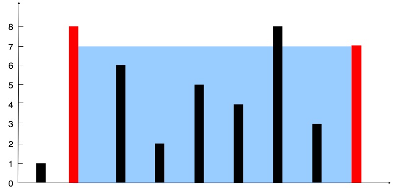
Input: height = [1,8,6,2,5,4,8,3,7] Output: 49 Explanation: The above vertical lines are represented by array [1,8,6,2,5,4,8,3,7]. In this case, the max area of water (blue section) the container can contain is 49.
Example 2:
Input: height = [1,1] Output: 1
Constraints:
n =height.length=2 <n <= 10=50 <height[i] <= 10=4
※ 2.3.4.1. Constraints and Edge Cases
- we need to pick two possible locations for container walls, the other walls don’t exist yet, they are just options
- we need to just return the max value, no indices needed
※ 2.3.4.2. My Solution (Code)
※ 2.3.4.2.1. My failed solution
I couldn’t figure out anything better than an \(O(n^2)\) even though this is CORRECT. Some of the testcases pass but the larger inputs have time limit exceeded – this is not fast enough.
1: class Solution: 2: │ def maxArea(self, height: List[int]) -> int: 3: │ │ maxFound = -float('inf') 4: │ │ for left in range(len(height) - 1): 5: │ │ │ for right in range(left + 1, len(height)): 6: │ │ │ │ if left == right: 7: │ │ │ │ │ continue 8: │ │ │ │ dx = right - left 9: │ │ │ │ minHeight = min(height[left], height[right]) 10: │ │ │ │ area = dx * minHeight 11: │ │ │ │ maxFound = max(area, maxFound) 12: │ │ │ │ 13: │ │ return maxFound
This other attempt tries to use two pointers, but the logic for moving them is off; it doesn’t guarantee all possible relevant areas are checked ==> not fair for searching This one doesn’t work and it’s not correct:
1: class Solution: 2: │ def maxArea(self, height: List[int]) -> int: 3: │ │ left, right = 0, len(height) - 1 4: │ │ maxFound = -float('inf') 5: │ │ findArea = lambda left, right: (min(height[left], height[right])) * (right - left ) 6: │ │ currentArea = findArea(left, right) 7: │ │ maxFound = currentArea 8: │ │ while(left < right): 9: │ │ │ leftShiftPossible = findArea(left + 1, right) 10: │ │ │ if(leftShiftPossible > currentArea): 11: │ │ │ │ left += 1 12: │ │ │ │ maxFound = leftShiftPossible 13: │ │ │ │ continue 14: │ │ │ │ 15: │ │ │ rightShiftPossible = findArea(left, right - 1) 16: │ │ │ if (rightShiftPossible > currentArea ): 17: │ │ │ │ right -= 1 18: │ │ │ │ maxFound = rightShiftPossible 19: │ │ │ │ continue 20: │ │ │ │ 21: │ │ │ left += 1 22: │ │ │ right -= 1 23: │ │ │ 24: │ │ return maxFound
※ 2.3.4.2.2. Optimal: Greedy, 2 pointer solution
The optimal solution uses 2 converging pointers, one at each end of the array.
- Moving the taller line inward can’t increase the area because the width shrinks and the height can’t increase. This is because the shorter line is the bottleneck.
- If we move the shorter line, we might find a taller line that might have more pros-than-cons-of-moving
- So we should move the pointer that is pointing to the shorter line and move it inwards.
At each step, we greedily discard the shorter wall, because keeping it can’t possibly help us form a larger area in the future.
Here’s the complete solution:
1: class Solution: 2: def maxArea(self, height: List[int]) -> int: 3: 4: left, right = 0, len(height) - 1 5: max_area = 0 6: 7: # greedily explore using 2 pointers: 8: while left < right: 9: │ │ curr_area = (right - left) * min(height[left], height[right]) 10: │ │ max_area = max(max_area, curr_area) 11: │ │ 12: │ │ # we always try to go for the best current step. current step is limited by the smaller one, so we try to pick a bigger guy for it. 13: │ │ # find the limiting factor and adjust: 14: │ │ if height[left] < height[right]: 15: │ │ left += 1 16: │ │ else: 17: │ │ right -= 1 18: │ │ 19: return max_area
※ 2.3.4.3. My Approach/Explanation
Here’s the stuff I do know:
- the use of “water” is intentional, but in this case the pillars don’t pre-exist so we don’t need to care about a subset area filling up differently from the rest
- The analogy for this is like that of a rubberband iirc, but I can’t imagine how the searching would be fair or how to make the right greedy judgement
- As a 2-pointer solution, we expect the performance to be \(O(n)\) speed and \(O(1)\) space
- I know that it’s greedily decided but What I’m missing is the greedy insight: when do we restrict?
※ 2.3.4.4. My Learnings/Questions
- is this even greedily determined?
- the init for a max accumulating variable doesn’t always have to be
-float('int'). In this case, because it’s array and that value can’t be negative, then we can set the initial value to 0. - We can actually just focus on finding out what the greedy property would be – how to make the best locally good decision? That should give us insight.
- the point on different approaches: Are There Completely Different Approaches? Data structures: No. There is no known O(n log n) or O(n) solution using stacks, heaps, or segment trees for this problem. The two-pointer greedy approach is optimal. Why not DP? The problem’s structure doesn’t allow for meaningful subproblem reuse. Why not monotonic stack? That’s useful for “largest rectangle in histogram” but not here, because both endpoints are variable.
※ 2.3.5. [14] Trapping Rainwater (42) hard redo
Given n non-negative integers representing an elevation map where the
width of each bar is 1, compute how much water it can trap after
raining.
Example 1:
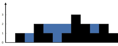
Input: height = [0,1,0,2,1,0,1,3,2,1,2,1] Output: 6 Explanation: The above elevation map (black section) is represented by array [0,1,0,2,1,0,1,3,2,1,2,1]. In this case, 6 units of rain water (blue section) are being trapped.
Example 2:
Input: height = [4,2,0,3,2,5] Output: 9
Constraints:
n =height.length=1 <n <= 2 * 10=40 <height[i] <= 10=5
This threw me off guard the previous time I saw this and I hadn’t internalised the main parts of this. Refer to the writeup here.
※ 2.3.5.1. Constraints and Edge Cases
- they aren’t asking to pick some optimal state, it’s about accumulating some water and geting the most amount out
※ 2.3.5.2. My Solution (Code)
※ 2.3.5.2.1. v0: correct, inferior \(O(n)\) time, \(O(n)\) space solution:
This just does prefix sums leftward and rightward.
1: class Solution: 2: │ def trap(self, height: List[int]) -> int: 3: │ │ if not height: 4: │ │ │ return 5: │ │ │ 6: │ │ n = len(height) 7: │ │ left_maxes, right_maxes = [0] * n, [0] * n 8: │ │ 9: │ │ for i in range(n): 10: │ │ │ prev_max = left_maxes[i - 1] if i - 1 >= 0 else 0 11: │ │ │ left_maxes[i] = max(prev_max, height[i]) 12: │ │ │ 13: │ │ # right maxes, we accumulate from right to left 14: │ │ for i in range(n - 1, - 1, -1): 15: │ │ │ next_max = right_maxes[i + 1] if i + 1 < n else 0 16: │ │ │ right_maxes[i] = max(next_max, height[i]) 17: │ │ │ 18: │ │ accum = 0 19: │ │ 20: │ │ for idx, (left_max, right_max) in enumerate(zip(left_maxes, right_maxes)): 21: │ │ │ valley_height = height[idx] 22: │ │ │ limiting = min(left_max, right_max) 23: │ │ │ accum += limiting - valley_height 24: │ │ │ 25: │ │ return accum
※ 2.3.5.2.2. v1: Ideal optimal \(O(n)\) time, \(O(1)\) space solution
1: class Solution: 2: │ def trap(self, height: List[int]) -> int: 3: │ │ if not height: 4: │ │ │ return 0 5: │ │ │ 6: │ │ left, right = 0, len(height) - 1 7: │ │ max_left, max_right = height[left], height[right] 8: │ │ 9: │ │ accumulated = 0 # nothing to accumulate at the edges 10: │ │ 11: │ │ while left < right: 12: │ │ │ is_left_limiting = max_left < max_right 13: │ │ │ if is_left_limiting: # should constrict left side 14: │ │ │ │ left += 1 15: │ │ │ │ max_left = max(max_left, height[left]) 16: │ │ │ │ # matters less if hte current left is higher than previous known bound -- it's just gonna be change = 0 17: │ │ │ │ change = max_left - height[left] 18: │ │ │ │ accumulated += max(0, change) 19: │ │ │ else: 20: │ │ │ │ right -= 1 21: │ │ │ │ max_right = max(max_right, height[right]) 22: │ │ │ │ change = max_right - height[right] 23: │ │ │ │ accumulated += max(0, change) 24: │ │ │ │ 25: │ │ return accumulated
This is after a bit of hand-holding from before, I need to redo this again. This solution runs in \(O(n)\) time because each index is visited at most once. The space usage is in \(O(1)\) because it’s all in place and fixed variables used for tracking.
※ 2.3.5.3. My Approach/Explanation
- Need to figure out when water gets trapped:
- when it’s within a valley
- the amount of water depends on the best height to the right and the best height to the left – how deep the valley is so for any particular spot, we need to keep track of max left and max right ( to find out how deep the valley is)
- we measure the accumulation by accumulating block by block so for each block
iwhat the water level is going to be above it. - water level above block
iis determined by the shorter of these two max blocks (max left, max right)
※ 2.3.5.4. My Learnings/Questions
- learning: the empty cases can really just be early returned – this helps improve timings compared to the population.
- Don’t get stumped by the related questions on this. The question was to find total accumulation, not the best choice or biggest valley. This means the success rate for each question is still based on the ability to break it down, not some guesswork.
Alternative approaches: Stack-based: As above, this approach is more general and useful for histogram problems, but for this specific problem, the two-pointer approach is preferred for its O(1) space
DP with precomputed arrays: Useful if you need to know left/right max for each position for other reasons, but not as space-efficient as two pointers
Precompute Left/Right Max Arrays (DP)
Idea: For each position, precompute the tallest bar to the left and right.
Time: O(n)
Space: O(n) (for two extra arrays)
How:
Scan left-to-right to fill leftmax[i].
Scan right-to-left to fill rightmax[i].
For each position, trapped water is min(leftmax[i], rightmax[i]) - height[i]
.
Stack-Based Solution
Idea: Use a stack to keep track of bars that are bounded by taller bars.
Time: O(n)
Space: O(n)
How:
Iterate through the array.
When you find a bar taller than the bar at the top of the stack, pop from the stack and calculate trapped water
.
※ 2.3.5.5. Retros
※ 2.3.5.5.1.
As usual, for the hard retros, I’m just focusing on getting the right answer out, instead of the perfect answer.
This made me focus on the basic preprocessed approach which does the prefix max from left and right and then calculates things.
1: class Solution: 2: │ def trap(self, height: List[int]) -> int: 3: │ │ if not height: 4: │ │ │ return 5: │ │ │ 6: │ │ n = len(height) 7: │ │ left_maxes, right_maxes = [0] * n, [0] * n 8: │ │ 9: │ │ for i in range(n): 10: │ │ │ prev_max = left_maxes[i - 1] if i - 1 >= 0 else 0 11: │ │ │ left_maxes[i] = max(prev_max, height[i]) 12: │ │ │ right = n - i - 1 13: │ │ │ next_max = right_maxes[right + 1] if right + 1 < n else 0 14: │ │ │ right_maxes[right] = max(next_max, height[right]) 15: │ │ │ 16: │ │ accum = 0 17: │ │ 18: │ │ for idx, (left_max, right_max) in enumerate(zip(left_maxes, right_maxes)): 19: │ │ │ valley_height = height[idx] 20: │ │ │ limiting = min(left_max, right_max) 21: │ │ │ accum += limiting - valley_height 22: │ │ │ 23: │ │ return accum 24:
Here’s the 2 pointer solution again:
1: class Solution: 2: │ def trap(self, height: List[int]) -> int: 3: │ │ if not height: 4: │ │ │ return 5: │ │ │ 6: │ │ left, right = 0, len(height) - 1 7: │ │ max_left, max_right = height[left], height[right] 8: │ │ 9: │ │ accum = 0 10: │ │ 11: │ │ while left < right: 12: │ │ │ # if left is shorter, then instead of the right boundary, this is the one that is limiting it 13: │ │ │ if is_left_shorter:=(max_left < max_right): 14: │ │ │ │ left += 1 # we compare the immediate next to the limited boundary: 15: │ │ │ │ max_left = max(max_left, height[left]) 16: │ │ │ │ valley_depth = max_left - height[left] 17: │ │ │ │ accum += max(valley_depth, 0) 18: │ │ │ else: 19: │ │ │ │ # mirror 20: │ │ │ │ right -= 1 # compare the immediate next to the limited boundary 21: │ │ │ │ max_right = max(max_right, height[right]) 22: │ │ │ │ valley_depth = max_right - height[right] 23: │ │ │ │ accum += max(valley_depth, 0) 24: │ │ │ │ 25: │ │ return accum
- At every iteration, you’re standing at
leftandright.- Whichever side currently has a lower max so far (
max_left < max_right), that side is the limiting wall for any valley between the pointers. - You want to process (potentially trap water at) the next cell from the lower wall because only as you step into it will you know how much is trapped above it.
- Whichever side currently has a lower max so far (
Invariant:
For the side currently being incremented, all prior cells up to that new pointer have already been compared to a wall at least as high as their own value.
※ 2.4. Stack
| Headline | Time | ||
|---|---|---|---|
| Total time | 4:54 | ||
| Stack | 4:54 | ||
| [15] Valid Parentheses (20) | 0:17 | ||
| [16] Min Stack (155) | 0:26 | ||
| [17] Evaluate Reverse Polish Notation… | 0:36 | ||
| [18] Generate Parentheses (22) | 1:01 | ||
| [19] Daily Temperatures (739) | 1:06 | ||
| [20] Car Fleet (853) | 0:28 | ||
| [21] Largest Rectangle in Histogram (84) | 1:00 |
※ 2.4.1. General Notes
※ 2.4.1.1. Fundamentals
- General Intuition on Monotonic stack pattern.
It seems that usually, the in-consideration elements are the ones that we’re putting in the stack. They’re in there because we need to preserve some intermediate order of these in-consideration elements.
- in some cases, we’re putting the unresolved elements in the monotonic stack.
- this is also useful when we want to keep a history of considerations while we find boundaries for things. The history point rings true here.
the stack could also be the currently accumulated best value (e.g. like in the remove duplicates question)
Show/Hide Md Code│ Your intuition is exactly right, and it’s echoed in the literature on monotonic stacks: │ │ - **The stack holds "unresolved" elements**—those for which you haven’t yet found the next smaller (or greater) element. │ - **History preservation:** The stack acts as a memory of the indices (or values) of elements that are still "waiting" for their boundary to be found. As you process each new element, you check if it resolves the boundary for any of the elements in the stack[1][2][3]. │ │ ### Why keep unresolved elements in the stack? │ - **Boundary finding:** For problems like "next smaller/greater element," you need to know, for each element, when a boundary (i.e., a smaller/greater bar) is encountered. You can't know this until you see a bar that breaks the monotonic property. │ - **Efficient processing:** By keeping a stack of unresolved elements, you process each element only when its boundary is found, ensuring O(n) time[1][2][3]. │ - **Order preservation:** The stack maintains a partial order (monotonically increasing or decreasing), which is crucial for efficiently determining boundaries. │ │ ### Example: Largest Rectangle in Histogram │ - As you sweep through the histogram, each bar is pushed onto the stack if it hasn't yet found a right boundary (a bar shorter than itself). │ - When you find a shorter bar, you pop from the stack, resolving the right boundary for the popped bar. The element below in the stack is the left boundary. │ - The stack thus "remembers" all the bars for which you haven't yet found a right boundary. │ │ > “Monotonic stacks are ideal for problems where you need to find the ‘next’ element based on specific criteria, like the next greater element. They are also effective for dynamically maintaining the maximum or minimum element in a changing window. ... By dynamically removing irrelevant elements and preserving a monotonic order, they enable efficient solutions to problems that might otherwise be much slower.”[2] │ │ ### General Principle │ - **The stack is a history of candidates**: It holds all elements still waiting for their answer (boundary), and as soon as the answer is found, they're popped and processed. │ - **This pattern is powerful** for a wide range of problems involving "next" or "previous" constraints (e.g., next greater/smaller, sliding window maximum/minimum)[1][2][3]. │ │ **References:** │ [1] algo.monster: Monotonic Stack/Queue Intro │ [2] teddysmith.io: Simplify Algorithm Design with the Monotonic Stack Pattern │ [3] GeeksforGeeks: Introduction to Monotonic Stack │ │ [1] https://algo.monster/problems/mono_stack_intro │ [2] https://teddysmith.io/monotonic-stack-algorithm-pattern/ │ [3] https://www.geeksforgeeks.org/dsa/introduction-to-monotonic-stack-2/ │ [4] https://en.wikipedia.org/wiki/Sorting_algorithm │ [5] https://stackoverflow.com/questions/72625101/how-do-i-solve-it-with-a-monotonic-stack │ [6] https://labuladong.online/algo/en/data-structure/monotonic-stack/ │ [7] https://en.wikipedia.org/wiki/Monotonic_function │ [8] https://liuzhenglaichn.gitbook.io/algorithm/monotonic-stack │ [9] https://blog.devgenius.io/monotonic-stack-algorithm-pattern-7bfac59157c2?gi=5dccec2461a5 │ [10] https://stackoverflow.com/questions/77878403/finding-all-sequences-with-same-stack-operations-to-make-monotonic-stack-from-th
※ 2.4.1.2. Tricks
※ 2.4.1.3. Sources of Error
remember to allow every option to be considered (e.g. to be inserted into the monotonic stack). If necessary, we can intentionally iterate until out of range and add a sentinel value for our ease.
This point comes from how we did so for the largest rectangle question.
GOTCHA: division “truncates towards zero”
One pitfall is in not realising the division is described to be “tend to zero” instead of “tend to infinity” In Python, / does floor division, which always rounds towards negative infinity. The problem statement for Evaluate Reverse Polish Notation (LeetCode 150) specifies that division between two integers should truncate towards zero, not negative infinity. For example, =-7 / 2
= -4, but the answer should be-3.We can do this instead:
'/': lambda a, b: int(a / b) # IMPORTANT:truncates towards zero
※ 2.4.2. [15] Valid Parentheses (20)
Given a string s containing just the characters '(', ')', '{',
'}', '[' and ']', determine if the input string is valid.
An input string is valid if:
- Open brackets must be closed by the same type of brackets.
- Open brackets must be closed in the correct order.
- Every close bracket has a corresponding open bracket of the same type.
Example 1:
Input: s = “()”
Output: true
Example 2:
Input: s = “()[]{}”
Output: true
Example 3:
Input: s = “(]”
Output: false
Example 4:
Input: s = “([])”
Output: true
Constraints:
1 <s.length <= 10=4sconsists of parentheses only'()[]{}'.
※ 2.4.2.1. Constraints and Edge Cases
- they give us the matching algo already, we just have to implement it
※ 2.4.2.2. My Solution (Code)
※ 2.4.2.2.1. v0 optimal solution
1: class Solution: 2: │ def isValid(self, s: str) -> bool: 3: │ │ openerToCloser = {'(': ')', '{' : '}', '[': ']' } 4: │ │ openers = openerToCloser.keys() 5: │ │ closers = openerToCloser.values() 6: │ │ 7: │ │ # a list is fine here, append and pop run in O(1) 8: │ │ stack = [] 9: │ │ for elem in s: 10: │ │ │ if len(stack) == 0 and elem in closers: 11: │ │ │ │ return False 12: │ │ │ │ 13: │ │ │ if len(stack) == 0 and elem in openers: 14: │ │ │ │ stack.append(elem) 15: │ │ │ │ continue 16: │ │ │ │ 17: │ │ │ │ 18: │ │ │ # non-empty stack cases: 19: │ │ │ if elem in closers: 20: │ │ │ │ is_matching_bracket = elem == openerToCloser[stack.pop()] 21: │ │ │ │ if is_matching_bracket: 22: │ │ │ │ │ continue 23: │ │ │ │ else: # found mismatch 24: │ │ │ │ │ return False 25: │ │ │ │ │ 26: │ │ │ if elem in openers: 27: │ │ │ │ stack.append(elem) 28: │ │ │ │ continue 29: │ │ │ │ 30: │ │ return not stack
※ 2.4.2.3. My Approach/Explanation
- There’s already a hint that the order of insertion matters. More specifically, we need to match the most recently inserted bracket. This hints at the FILO nature which then shows us a stack needs to be used.
- For the bracket matching, there’s a need to represent the relationship between an opener and its corresponding closer. We can reuse the keys and values (as well as the dictionary itself) for lookup purposes.
※ 2.4.2.4. My Learnings/Questions
interesting empirical learning: the time was faster when I convert things to lists instead of using keys and values in their own objects.
Based on my language understandings, this doesn’t matter.
This means that:
this was slow
Show/Hide Python Code│ │ openers = openerToCloser.keys() │ │ closers = openerToCloser.values()
this was fast:
Show/Hide Python Code│ │ openers = list(openerToCloser.keys()) │ │ closers = list(openerToCloser.values())
Our stack only keeps a single kind of thing: the openers.
Closers are never added in.
※ 2.4.3. [16] Min Stack (155)
Design a stack that supports push, pop, top, and retrieving the minimum element in constant time.
Implement the MinStack class:
MinStack()initializes the stack object.void push(int val)pushes the elementvalonto the stack.void pop()removes the element on the top of the stack.int top()gets the top element of the stack.int getMin()retrieves the minimum element in the stack.
You must implement a solution with O(1) time complexity for each
function.
Example 1:
Input ["MinStack","push","push","push","getMin","pop","top","getMin"] [[],[-2],[0],[-3],[],[],[],[]] Output [null,null,null,null,-3,null,0,-2] Explanation MinStack minStack = new MinStack(); minStack.push(-2); minStack.push(0); minStack.push(-3); minStack.getMin(); // return -3 minStack.pop(); minStack.top(); // return 0 minStack.getMin(); // return -2
Constraints:
-2=^{=31}= <= val <= 2=31= - 1=- Methods
pop,topandgetMinoperations will always be called on non-empty stacks. - At most
3 * 10=^{=4} calls will be made topush,pop,top, andgetMin.
※ 2.4.3.1. Constraints and Edge Cases
Nothing fancy.
※ 2.4.3.2. My Solution (Code)
※ 2.4.3.2.1. v0: correct \(O(1)\) time, \(O(n)\) space
This is my approach. It runs in \(O(1)\) time and \(O(n)\) space (at worst case, where in every value is a new minimum val)
1: class MinStack: 2: │ 3: │ def __init__(self): 4: │ │ self.stack = [] 5: │ │ self.minVals = [] 6: │ │ 7: │ def push(self, val: int) -> None: 8: │ │ # based on constraint, whereby push() may be called on empty stack 9: │ │ is_first_val = not self.stack and not self.minVals 10: │ │ if (is_first_val): 11: │ │ │ self.stack.append(val) 12: │ │ │ self.minVals.append(val) 13: │ │ │ 14: │ │ │ return 15: │ │ │ 16: │ │ self.stack.append(val) 17: │ │ is_new_min = val <= self.minVals[-1] 18: │ │ if is_new_min: 19: │ │ │ self.minVals.append(val) 20: │ │ │ 21: │ │ return 22: │ │ 23: │ def pop(self) -> None: 24: │ │ popped = self.stack.pop() 25: │ │ is_popping_min = popped == self.minVals[-1] 26: │ │ 27: │ │ if is_popping_min: 28: │ │ │ self.minVals.pop() 29: │ │ │ 30: │ │ return 31: │ │ 32: │ def top(self) -> int: 33: │ │ return self.stack[-1] 34: │ │ 35: │ def getMin(self) -> int: 36: │ │ return self.minVals[-1]
This is a cleaner approach:
1: class MinStack: 2: │ def __init__(self): 3: │ │ self.stack = [] 4: │ │ self.minVals = [] 5: │ │ 6: │ def push(self, val: int) -> None: 7: │ │ self.stack.append(val) 8: │ │ if not self.minVals or val <= self.minVals[-1]: 9: │ │ │ self.minVals.append(val) 10: │ │ │ 11: │ def pop(self) -> None: 12: │ │ if self.stack: 13: │ │ │ popped = self.stack.pop() 14: │ │ │ if popped == self.minVals[-1]: 15: │ │ │ │ self.minVals.pop() 16: │ │ │ │ 17: │ def top(self) -> int: 18: │ │ return self.stack[-1] 19: │ │ 20: │ def getMin(self) -> int: 21: │ │ return self.minVals[-1]
※ 2.4.3.2.2. v1: space optimised, single stack
This is an optimisation that uses a single stack and we use a tuple of (val, minsofar):
1: class MinStack: 2: │ def __init__(self): 3: │ │ self.stack = [] 4: │ │ 5: │ def push(self, val: int) -> None: 6: │ │ min_so_far = val if not self.stack else min(val, self.stack[-1][1]) 7: │ │ self.stack.append((val, min_so_far)) 8: │ │ 9: │ def pop(self) -> None: 10: │ │ self.stack.pop() 11: │ │ 12: │ def top(self) -> int: 13: │ │ return self.stack[-1][0] 14: │ │ 15: │ def getMin(self) -> int: 16: │ │ return self.stack[-1][1]
※ 2.4.3.3. My Approach/Explanation
- Since everything is in \(O(1)\) time, it means that we need to use aux datastructures well.
- A list will function alright as a stack unless we do any shifting.
- we don’t expect any shifting to be done though
- This aligns with the “history” stack approach where we think of doing undos/keeping track of history of something. We then need to just find out what that thing is that we need to keep track of.
- Now, we realise that there’s a FILO behaviour done on two things :
- the order at which new minimum values show up: the most recent min value (appropriate for the current history state) needs to be out first
- the order at which values are kept: the most recent insertion needs to be out first
※ 2.4.3.4. My Learnings/Questions
- I think I should have got this faster. I actually ended up iterating on things as the realisations came. Still a morale boost though.
※ 2.4.4. [17] Evaluate Reverse Polish Notation (150)
You are given an array of strings tokens that represents an arithmetic
expression in a
Reverse Polish
Notation.
Evaluate the expression. Return an integer that represents the value of the expression.
Note that:
- The valid operators are
'+','-','*', and'/'. - Each operand may be an integer or another expression.
- The division between two integers always truncates toward zero.
- There will not be any division by zero.
- The input represents a valid arithmetic expression in a reverse polish notation.
- The answer and all the intermediate calculations can be represented in a 32-bit integer.
Example 1:
Input: tokens = ["2","1","+","3","*"] Output: 9 Explanation: ((2 + 1) * 3) = 9
Example 2:
Input: tokens = ["4","13","5","/","+"] Output: 6 Explanation: (4 + (13 / 5)) = 6
Example 3:
Input: tokens = ["10","6","9","3","+","-11","*","/","*","17","+","5","+"] Output: 22 Explanation: ((10 * (6 / ((9 + 3) * -11))) + 17) + 5 = ((10 * (6 / (12 * -11))) + 17) + 5 = ((10 * (6 / -132)) + 17) + 5 = ((10 * 0) + 17) + 5 = (0 + 17) + 5 = 17 + 5 = 22
Constraints:
1 <tokens.length <= 10=4tokens[i]is either an operator:"+","-","*", or"/", or an integer in the range[-200, 200].
※ 2.4.4.1. Constraints and Edge Cases
- we don’t need to handle adversarial edge cases here.
- GOTCHA: One pitfall is in not realising the division is described to be “tend to zero” instead of “tend to infinity”
In Python, / does floor division, which always rounds towards negative infinity.
The problem statement for Evaluate Reverse Polish Notation (LeetCode 150) specifies that division between two integers should truncate towards zero, not negative infinity.
For example, =-7 / 2
= -4, but the answer should be-3. - Also careful in determining the right vs left operands, the examples actually clarify this, I think these are the areas that can throw someone off-guard since it’s really a nit and it’s easy to change the question based on this.
- We don’t need to handle negative tokens.
- We can assume that all the operations are binary operations.
※ 2.4.4.2. My Solution (Code)
Here’s my solution. It has some inefficiencies because of the type conversions that we’re doing, we can just default all to integers @ first-parse. This solution runs in \(O(n)\) time (each token processed only once) and \(O(n)\) space (the stack can grow up to n/2 for worst case where all the operands show up before the operators)
1: class Solution: 2: │ def evalRPN(self, tokens: List[str]) -> int: 3: │ │ fns = { 4: │ │ │ "+": lambda a, b: str(int(a) + int(b)), 5: │ │ │ "-": lambda a, b: str(int(a) - int(b)), 6: │ │ │ "*": lambda a, b: str(int(a) * int(b)), 7: │ │ │ "/": lambda a, b: str(int(int(a) / int(b))), 8: │ │ │ } 9: │ │ │ 10: │ │ stack = [] 11: │ │ for token in tokens: 12: │ │ │ if token not in fns: 13: │ │ │ │ stack.append(token) 14: │ │ │ else: 15: │ │ │ │ # assumption: it's all binary fns: 16: │ │ │ │ right_operand = stack.pop() 17: │ │ │ │ left_operand = stack.pop() 18: │ │ │ │ result = fns[token](int(left_operand), int(right_operand)) 19: │ │ │ │ stack.append(str(result)) 20: │ │ │ │ 21: │ │ return int(stack[0])
The following is a cleaner solution. It avoids the overheads due to consistent type conversions.
1: class Solution: 2: │ def evalRPN(self, tokens: List[str]) -> int: 3: │ │ fns = { 4: │ │ │ '+': lambda a, b: a + b, 5: │ │ │ '-': lambda a, b: a - b, 6: │ │ │ '*': lambda a, b: a * b, 7: │ │ │ '/': lambda a, b: int(a / b) # IMPORTANT:truncates towards zero 8: │ │ } 9: │ │ stack = [] 10: │ │ for token in tokens: 11: │ │ │ if token in fns: 12: │ │ │ │ b = stack.pop() 13: │ │ │ │ a = stack.pop() 14: │ │ │ │ stack.append(fns[token](a, b)) 15: │ │ │ else: 16: │ │ │ │ stack.append(int(token)) 17: │ │ return stack[0]
Extra: this is a recursive variant but it is less efficient
Certainly! Here’s a **recursive variant** for evaluating Reverse Polish Notation (RPN): ## Recursive RPN Evaluation The idea is to process the tokens from the end (rightmost), since in RPN the last element is either an operand (final result) or an operator whose operands come before it. Each time you encounter an operator, recursively evaluate its two operands. ### Implementation ```python class Solution: │ def evalRPN(self, tokens: List[str]) -> int: │ │ def helper(index: int) -> (int, int): │ │ │ token = tokens[index] │ │ │ if token not in {"+", "-", "*", "/"}: │ │ │ │ return int(token), index - 1 │ │ │ │ │ │ │ # Recursively evaluate right and left operands │ │ │ right, idx = helper(index - 1) │ │ │ left, idx = helper(idx) │ │ │ │ │ │ if token == "+": │ │ │ │ return left + right, idx │ │ │ elif token == "-": │ │ │ │ return left - right, idx │ │ │ elif token == "*": │ │ │ │ return left * right, idx │ │ │ else: # division, truncate towards zero │ │ │ │ return int(left / right), idx │ │ │ │ │ │ result, _ = helper(len(tokens) - 1) │ │ return result ``` ### How it works - The helper function processes tokens from the end. - If the token is a number, return its value and the new index. - If the token is an operator, recursively evaluate the right and left operands (note the order: right first, then left). - Each recursive call returns the computed value and the next index to process. ### Example For `tokens = ["2", "1", "+", "3", "*"]`: - `helper(4)` sees `"*"`, so it recursively evaluates operands at `3` and before. - This continues until all numbers and operations are processed. ### Notes - This approach is elegant but less efficient than the stack-based approach, due to recursion and function call overhead. - Python’s default recursion limit may be exceeded for very large inputs. **Let me know if you want a step-by-step trace or have questions about recursion in RPN!**
※ 2.4.4.3. My Approach/Explanation
Keep a map of functions that we wanna handle and the lambdas for them. Only add in the actual operands, not the operators to the stack. Since it’s binary only, it’s easier to handle since we don’t need to account for brackets as tokens.
※ 2.4.4.4. My Learnings/Questions
- Deque: You could use collections.deque as a stack, but Python’s list is already optimized for stack operations.
- things like the order of operands can possibly be simple ways that someone can change the question and throw you offguard, I think these aspecs should always be verified.
- Stack is optimised for RPN.
※ 2.4.5. [18] ⭐️ Generate Parentheses (22) med redo backtracking combinations
Given n pairs of parentheses, write a function to generate all
combinations of well-formed parentheses.
Example 1:
Input: n = 3 Output: ["((()))","(()())","(())()","()(())","()()()"]
Example 2:
Input: n = 1 Output: ["()"]
Constraints:
1 <n <= 8=
※ 2.4.5.1. Constraints and Edge Cases
they gave a small number
1<=n<=8for a reason. It’s because it’s combination finding, which means the number of combinations at most is the catalan number \(O(4^{n}/sqrt(n))\).Combination finding here is essentially just a brute force, backtracking without much pruning.
※ 2.4.5.2. My Solution (Code)
See other solutions below
※ 2.4.5.2.1. v0: failed solution
I think I have the gist of how to do it but I don’t really know. Here’s the current working so far:
1: class Solution: 2: │ def generateParenthesis(self, n: int) -> List[str]: 3: │ │ def helper(combis, n) : 4: │ │ │ if n <= 0: 5: │ │ │ return combis 6: │ │ │ else: 7: │ │ │ new_combis = [] 8: │ │ │ for accum, stack in combis: 9: │ │ │ │ # if stack is empty, I can only add new brace. then decide what to w its partner: add first or add later: 10: │ │ │ │ if not stack: 11: │ │ │ │ │ # choice A: yes to opener, no to closer 12: │ │ │ │ │ new_combis.append((accum.copy() + "(", stack.copy().append(")"))) 13: │ │ │ │ │ # choice B: yes to opener and closer 14: │ │ │ │ │ new_combis.append((accum.copy() + "()", stack.copy())) 15: │ │ │ │ else: 16: │ │ │ │ │ 17: │ │ │ │ │ # choice C: for first char, take closer from stack 18: │ │ │ │ │ c_stack = stack.copy() 19: │ │ │ │ │ c_accum = accum.copy() + c1_stack[-1] 20: │ │ │ │ │ c_stack.pop() 21: │ │ │ │ │ # C1: choice A and choice C 22: │ │ │ │ │ new_combis.append(c_accum.copy() + "(", c_stack.copy().append(")")) 23: │ │ │ │ │ 24: │ │ │ │ │ # C2: choice A and choice C 25: │ │ │ │ │ new_combis.append(c_accum.copy() + "()", c_stack.copy()) 26: │ │ │ │ │ 27: │ │ │ │ │ # choice D: for first char, do not take closer from stack 28: │ │ │ │ │ d_stack = stack.copy() 29: │ │ │ │ │ # D1: choice A and choice D 30: │ │ │ │ │ new_combis.append(accum.copy() + "(", d_stack.copy().append(")")) 31: │ │ │ │ │ # D2: choice A and choice D 32: │ │ │ │ │ new_combis.append(accum.copy() + "()", d_stack.copy()) 33: │ │ │ │ │ 34: │ │ │ return helper(new_combis, n-1) 35: │ │ │ 36: │ │ combis = helper([], n) 37: │ │ 38: │ │ return [com + "".join(stack) for com, stack in combis]
※ 2.4.5.2.2. v1: Backtracking Combinations Clean Solution
1: class Solution: 2: │ def generateParenthesis(self, n: int) -> List[str]: 3: │ │ res = [] 4: │ │ 5: │ │ def backtrack(curr, open_count, close_count): 6: │ │ │ if len(curr) == 2 * n: 7: │ │ │ │ res.append(curr) 8: │ │ │ │ return 9: │ │ │ if open_count < n: 10: │ │ │ │ backtrack(curr + "(", open_count + 1, close_count) 11: │ │ │ if close_count < open_count: 12: │ │ │ │ backtrack(curr + ")", open_count, close_count + 1) 13: │ │ │ │ 14: │ │ backtrack("", 0, 0) 15: │ │ return res
Idea:
- Only add
(if you have not yet used all opens. - Only add
)if there are more opens than closes so far. - Base case check: When the string is length
2n, it is a valid combination.
Complexity:
- runtime: \(O(4^n/\sqrt(n))\)
- space: \(O(n)\)
1: class Solution: 2: │ def generateParenthesis(self, n: int) -> List[str]: 3: │ │ res = [] 4: │ │ TOTAL = n * 2 5: │ │ 6: │ │ def backtrack(path, num_open, num_close): 7: │ │ │ # end states: 8: │ │ │ if len(path) == TOTAL: 9: │ │ │ │ res.append(path) 10: │ │ │ │ return 11: │ │ │ # choice type 1: 12: │ │ │ if should_add_closer:=(num_close < num_open): 13: │ │ │ │ backtrack(path + ")", num_open, num_close + 1) 14: │ │ │ │ 15: │ │ │ # choice type 2: 16: │ │ │ if should_add_opener:=(num_open < n): 17: │ │ │ │ backtrack(path + "(", num_open + 1, num_close) 18: │ │ │ │ 19: │ │ │ return 20: │ │ │ 21: │ │ backtrack("", 0, 0) 22: │ │ return res
※ 2.4.5.3. My Approach/Explanation
- I see how there’s a need to iterate down and there’s really 2 choices to make:
- add in a closer NOW or add it to stack. this can only be done if the stack is NOT empty
- what goes into the stack? only closers
- this choice-based thing makes me think that the simplest to reason with is a recursive solution
※ 2.4.5.4. My Learnings/Questions
- Sources of failure for the initial attempts:
- The use of .copy() and .append() in the same expression is problematic: .append() returns None, so stack.copy().append(“)”) is not valid Python.
- The code tries to manage a stack of closers and an accumulator, but the logic for generating valid combinations is convoluted and doesn’t properly enforce the rules for well-formed parentheses. The recursion and state management are much more complex than needed.
- theoretical approach to the optimal solution:
since this is about combinations, the number of valid combinations is the nth Catalan number. This makes the time and space usage both \(O(4^{n}/sqrt(n))\) Read more about catalan numbers here: Why is the constraint \(1 \leq n \leq 8\) important in the “generate parentheses” problem?
Show/Hide QuoteThe number of valid combinations of \(n\) pairs of parentheses is given by the Catalan number:
\[ C_n = \frac{1}{n+1}\binom{2n}{n} \]
The asymptotic growth of the Catalan numbers is:
\[ C_n \sim \frac{4^n}{n^{3/2}\sqrt{\pi}} \]
- This means the number of combinations grows very rapidly as \(n\) increases.
- For \(n=8\), \(C_8 = 1430\).
- For \(n=10\), \(C_{10} = 16796\).
- For \(n=15\), \(C_{15} = 9694845\) (almost 10 million!).
Therefore, the problem restricts \(n\) to small values because:
- The number of combinations is the Catalan number, which grows as \(O(4^n/\sqrt{n})\).
For large \(n\), generating and storing all combinations is computationally infeasible.
Summary: They gave a small number \(1 \leq n \leq 8\) for a reason. It’s because the number of valid combinations is the Catalan number, which grows as \(O(4^n/\sqrt{n})\). For large \(n\), the number of combinations becomes huge.
- Approach:
- instead of tracking closers ONLY, track the number of open and close parentheses used so far
- for efficiency, avoid copying strings or lists unnecessarily
- it’s definitely recursive because we’re doing combination-finding
- they’re calling it “Backtracking”:
- @ each step, we have 2 options which will still keep the rule:
- can add an opener if you haven’t used all the
nopeners - can add a closer if you haven’t used more closers than openers
- can add an opener if you haven’t used all the
- base case: when the size of the string is
2nthen we know both the openers and closers have all been used up
- @ each step, we have 2 options which will still keep the rule:
- Another thing is realised is that the approach is pretty single-minded. We don’t need to be convoluted in building things up then filtering them out if we can just build them while adhering to the rules.
- Python:
use string concatenation instead of needing to copy lists
Show/Hide Python Code1: s = "mystring" 2: copy = s 3: print(f"id(s): ${id(s)}") 4: print(f"id(copy): ${id(copy)}") 5: copy += "extension" 6: print(s) 7: print(copy) 8: print(f"id(s): ${id(s)}") 9: print(f"id(copy): ${id(copy)}") 10: # EXPLANATION: 11: # copy += "extension" does not modify the original string. 12: # Instead, it creates a new string object ("mystringextension") and assigns it to copy.
id(s): $4368497968 id(copy): $4368497968 mystring mystringextension id(s): $4368497968 id(copy): $4368162160
- Different approaches:
Iterative BFS: You can use a queue to build up valid combinations level by level, but recursion (backtracking) is more natural for this problem. We use a queue to build up valid combinations level by level. Each state in the queue tracks: the current string, the number of opens used, and the number of closes used.
Show/Hide Python Code1: from collections import deque 2: 3: class Solution: 4: │ def generateParenthesis(self, n: int) -> list[str]: 5: │ │ res = [] 6: │ │ queue = deque() 7: │ │ queue.append(("", 0, 0)) # (current_string, open_count, close_count) 8: │ │ 9: │ │ while queue: 10: │ │ │ curr, open_count, close_count = queue.popleft() 11: │ │ │ if len(curr) == 2 * n: 12: │ │ │ │ res.append(curr) 13: │ │ │ else: 14: │ │ │ │ if open_count < n: 15: │ │ │ │ │ queue.append((curr + "(", open_count + 1, close_count)) 16: │ │ │ │ if close_count < open_count: 17: │ │ │ │ │ queue.append((curr + ")", open_count, close_count + 1)) 18: │ │ return res
1-D Dynamic Programming: You can use DP to build up solutions for n from solutions for n-1, but backtracking is simpler and more direct. Sub-problem insight: We use the fact that a valid sequence for n pairs can be built by wrapping valid sequences of fewer pairs in a pair of parentheses and concatenating with others. This actually uses the recursive structure for Catalan numbers – Uses the recursive structure of Catalan numbers to build up solutions from smaller subproblems.
Show/Hide Python Code1: class Solution: 2: │ def generateParenthesis(self, n: int) -> list[str]: 3: │ │ dp = [[] for _ in range(n + 1)] 4: │ │ dp[0] = [""] 5: │ │ 6: │ │ for i in range(1, n + 1): 7: │ │ │ for j in range(i): 8: │ │ │ │ for left in dp[j]: 9: │ │ │ │ │ for right in dp[i - 1 - j]: 10: │ │ │ │ │ │ dp[i].append("(" + left + ")" + right) 11: │ │ return dp[n]
※ 2.4.5.5. Additional Context
I’m not sure why I struggled with this more than I expected to. On the plus side, I did get the correct intuition that it’s combinations-based so I need to do the recursive helper. Maybe the fact that this is grouped under “stack” for neetcode150 threw me off.
※ 2.4.5.6. Retros
※ 2.4.5.6.1.
This is morale-boosting.
It’s clear that I have to do a brute-force approach. So the backtracking approach is perfect here.
The backtracking framework (what’s the path, what’s the end states, what are the options to choose from? how many different types of choices to make in each iteration? how to avoid semantically similar things to avoid double counting?)
※ 2.4.6. [19] Daily Temperatures (739) med redo monotonic_stack
Given an array of integers temperatures represents the daily
temperatures, return an array answer such that answer[i] is the
number of days you have to wait after the i=^{=th} day to get a
warmer temperature. If there is no future day for which this is
possible, keep answer[i] = 0= instead.
Example 1:
Input: temperatures = [73,74,75,71,69,72,76,73] Output: [1,1,4,2,1,1,0,0]
Example 2:
Input: temperatures = [30,40,50,60] Output: [1,1,1,0]
Example 3:
Input: temperatures = [30,60,90] Output: [1,1,0]
Constraints:
1 <temperatures.length <= 10=530 <temperatures[i] <= 100=
※ 2.4.6.1. Constraints and Edge Cases
- need to return the num days until NEXT higher not the num days until the max temp
※ 2.4.6.2. My Solution (Code)
※ 2.4.6.2.1. v0 Failed attempts
The use of diffs and ranges is not a natural fit for the problem.
Your attempts are not correct for all cases. Both solutions try to use right-to-left sweeps and diffs, but do not efficiently or reliably find the next warmer day for each day. The logic for updating and tracking next peaks is convoluted and can produce wrong answers, especially for plateaus or multiple dips before the next rise.
initial right sweep attempt:
1: class Solution: 2: │ def dailyTemperatures(self, temperatures: List[int]) -> List[int]: 3: │ │ # just reverse the output 4: │ │ rev_accum = [(0, (temperatures[-1], temperatures[-1]))] 5: │ │ 6: │ │ for idx in range(len(temperatures) - 2, -1, -1): 7: │ │ │ curr_temp, prev_temp = temperatures[idx], temperatures[idx + 1] 8: │ │ │ prev_res, (low, high) = rev_accum[-1] 9: │ │ │ # out of range, too high: 10: │ │ │ if curr_temp > high: 11: │ │ │ │ rev_accum.append((0, (low, curr_temp))) 12: │ │ │ │ continue 13: │ │ │ │ 14: │ │ │ if curr_temp == prev_temp: 15: │ │ │ │ rev_accum.append((prev_res, (low, high))) 16: │ │ │ │ continue 17: │ │ │ │ 18: │ │ │ if curr_temp < prev_temp and curr_temp < low: 19: │ │ │ │ rev_accum.append((1, (curr_temp, high))) 20: │ │ │ │ continue 21: │ │ │ │ 22: │ │ │ # need to find the next highest, it's somewhere between: 23: │ │ │ res = 0 24: │ │ │ for find_idx in range(idx + 1, len(temperatures)): 25: │ │ │ │ if curr_temp < temperatures[find_idx]: 26: │ │ │ │ │ res = find_idx 27: │ │ │ │ │ break 28: │ │ │ rev_accum.append((res, (low, high))) 29: │ │ │ 30: │ │ rev_accum.reverse() 31: │ │ return [res for res, temp_range in rev_accum]
Complexity:
- time: Worst-case \(O(n^2)\) due to the inner loop searching for the next higher temperature
- space: \(O(n)\) for the result arrays
the following one is a diff check attempt. This is wrong. The logic for updating and tracking next peaks is convoluted and can produce wrong answers, especially for plateaus or multiple dips before the next rise.
- time: Also Worst-case \(O(n^2)\) as it may decrement and backtrack repeatedly.
- space: \(O(n)\) for the result arrays
1: class Solution: 2: │ def dailyTemperatures(self, temperatures: List[int]) -> List[int]: 3: │ │ res = [] 4: │ │ 5: │ │ # gather the diffs: 6: │ │ diffs = [] 7: │ │ for i in range(len(temperatures) - 1): 8: │ │ │ today, tmr = temperatures[i], temperatures[i + 1] 9: │ │ │ if tmr < today: 10: │ │ │ │ diffs.append(-1) 11: │ │ │ elif tmr > today: 12: │ │ │ │ diffs.append(1) 13: │ │ │ else: 14: │ │ │ │ diffs.append(0) 15: │ │ diffs.append(0) 16: │ │ 17: │ │ for i in range(len(diffs) - 1, -1, -1): 18: │ │ │ if i == len(diffs) - 1: 19: │ │ │ │ continue 20: │ │ │ │ 21: │ │ │ # ignore the 22: │ │ │ if diffs[i] == 1: 23: │ │ │ │ continue 24: │ │ │ │ 25: │ │ │ # current fella is 0: 26: │ │ │ j = i 27: │ │ │ while (left_is_non_positive:= j > 0 and diffs[j - 1] <= 0): 28: │ │ │ │ diffs[j - 1] -= 1 29: │ │ │ │ j -= 1 30: │ │ │ │ 31: │ │ │ diffs[i] -= 1 32: │ │ │ 33: │ │ return [abs(diff) for diff in diffs]
※ 2.4.6.2.2. v1: Optimal Solution monotonically increasing stack
Key Insight:
- each day we want to know the next day with higher temperature.
- A stack can keep track of indices of days with unresolved warmer days.
- Iterate left to right.
- For each temperature, while the stack is not empty and the current temperature is higher than the temperature at the index on top of the stack:
- Pop the index from the stack and set the result for that index to the current index minus the popped index.
- Push the current index onto the stack.
1: class Solution: 2: │ def dailyTemperatures(self, temperatures: List[int]) -> List[int]: 3: │ │ res = [0] * len(temperatures) 4: │ │ stack = [] # stores indices 5: │ │ 6: │ │ for i, temp in enumerate(temperatures): 7: │ │ │ while stack and temp > temperatures[stack[-1]]: 8: │ │ │ │ prev_idx = stack.pop() 9: │ │ │ │ distance = i - prev_idx 10: │ │ │ │ res[prev_idx] = distance 11: │ │ │ stack.append(i) 12: │ │ return res
Here’s the neetcode video for this to explain it.
the neetcode solution is a little easier to follow:
1: class Solution: 2: │ def dailyTemperatures(self, temperatures: List[int]) -> List[int]: 3: │ │ res = [0] * len(temperatures) 4: │ │ stack = [] # pair: (temp, index) 5: │ │ 6: │ │ for i, temp in enumerate(temperatures): 7: │ │ │ while stack and temp > stack[-1][0]: 8: │ │ │ │ stackTemp, stackIdx = stack.pop() 9: │ │ │ │ res[stackIdx] = i - stackIdx 10: │ │ │ stack.append((temp, i)) 11: │ │ │ 12: │ │ # NOTE: technically at this point the stack should have the ones for which there's no higher number. 13: │ │ # we can ignoer it because the res list already is all initialised to 0 14: │ │ return res
Time complexity: \(O(n)\) Space complexity: \(O(n)\)
I wrote this again.
1: class Solution: 2: │ def dailyTemperatures(self, temperatures: List[int]) -> List[int]: 3: │ │ res = [0] * len(temperatures) 4: │ │ stack = [] 5: │ │ for idx, temp in enumerate(temperatures): 6: │ │ │ if not stack: 7: │ │ │ │ stack.append((idx, temp)) 8: │ │ │ │ continue 9: │ │ │ │ 10: │ │ │ while can_conclude:=(stack and stack[-1][1] < temp): 11: │ │ │ │ start_idx, _ = stack.pop() 12: │ │ │ │ days = idx - start_idx 13: │ │ │ │ res[start_idx] = days 14: │ │ │ │ 15: │ │ │ stack.append((idx, temp)) 16: │ │ │ 17: │ │ return res
※ 2.4.6.2.3. 1-D DP Solution
1: class Solution: 2: │ def dailyTemperatures(self, temperatures: List[int]) -> List[int]: 3: │ │ n = len(temperatures) 4: │ │ res = [0] * n 5: │ │ # dp[i] is the number of days to wait until next warmer 6: │ │ 7: │ │ for i in range(n - 2, -1, -1): # go from right to left 8: │ │ │ j = i + 1 # right 9: │ │ │ # should skip ahead to find an appropriate j: 10: │ │ │ while j < n and temperatures[j] <= temperatures[i]: 11: │ │ │ │ if res[j] == 0: 12: │ │ │ │ │ j = n # no warmer temp ahead 13: │ │ │ │ │ break 14: │ │ │ │ j += res[j] # skips ahead, uses previously computed ans to pick next warmer candidate 15: │ │ │ │ 16: │ │ │ # found the right j 17: │ │ │ if j < n: 18: │ │ │ │ res[i] = j - i 19: │ │ return res
more elaboration on the dp approach:
Absolutely, let’s dig into the **Dynamic Programming approach** behind your solution for the Daily Temperatures problem: *** ## **Your Code (DP Style):** ```python class Solution: │ def dailyTemperatures(self, temperatures: List[int]) -> List[int]: │ │ n = len(temperatures) │ │ res = [0] * n │ │ for i in range(n - 2, -1, -1): # iterate from right to left │ │ │ j = i + 1 │ │ │ while j = n`), just return 0 for that day (no warm days ahead). │ │ │ *** ### **Alternative: Stack Approach** The most popular approach is a **monotonic stack**, which also achieves $$O(n)$$ time and is sometimes easier to code and reason for interview. In your DP approach, the skip-ahead logic is reminiscent of path compression in union-find. *** ### **Summary Table** | Approach | Key Idea | Time | Space | Implementation Notes | |------------------|------------------------------|---------|-------|--------------------------| | DP (yours) | Jump using earlier results | O(n) | O(n) | Right-to-left, uses res[] | | Stack (monotone) | Wait list for transitions | O(n) | O(n) | Left-to-right, uses stack | *** ### **Takeaways** - Your solution is correct, optimal, and a clever application of DP principles via answer propagation. - It highlights how DP isn’t always top-down/memoization: it’s any solution structure where you optimize by *building up answers to subproblems that benefit future queries*. If you want, I can show a visual/step-by-step walkthrough for a specific input or discuss the difference between this DP and the stack approach. Let me know! [1] https://ppl-ai-file-upload.s3.amazonaws.com/web/direct-files/collection_ef8c91e3-be4a-49b2-a82f-09d8f8cf21d9/2a8357be-5a6f-45ac-a67c-457cddf74a62/Variant-UnlimitedSupply-DPUpdatePattern-ExampleProblem.csv [2] https://www.educative.io/answers/daily-temperatures-leetcode [3] https://algo.monster/liteproblems/739 [4] https://leetcode.com/problems/daily-temperatures/ [5] https://www.youtube.com/watch?v=ekFs9Nb2RNQ [6] https://www.youtube.com/watch?v=_ZEvmycwXHs [7] https://teddysmith.io/daily-temperatures-739-leetcode-2/ [8] https://walkccc.me/LeetCode/problems/739/ [9] https://www.youtube.com/watch?v=KbxtI6kSLGI
Time complexity: \(O(n)\) Space complexity:
- \(O(1)\) extra space.
- \(O(n)\) space for the output array.
This is similar in intuition to my diff attempt in some ways.
Great question! Let’s break down **how this 1-D DP solution is similar to your attempts** and how it differs, with some intuition. ## 1. **Your Attempt: Diffs and Right Sweep** Your approach tried to: - Sweep from right to left. - For each day, somehow track the difference or "how many days" until a warmer temperature. - You tried to propagate or decrement differences, but the logic got convoluted and sometimes required O(n²) backtracking. ## 2. **The 1-D DP Solution:** This solution also: - Sweeps from right to left. - For each day, tries to efficiently "jump" ahead to the next warmer day, using previously computed results. ### **How it works:** - For each index `i`, you look at `j = i + 1`. - If `temperatures[j] > temperatures[i]`, you found the next warmer day. - If not, and if `res[j] > 0`, you can "jump" directly to `j + res[j]` (the next candidate warmer day), skipping over cold days in O(1) per jump. - If `res[j] == 0`, there is no warmer day ahead, so you can stop. - This is a form of **dynamic programming with memoization**: you reuse previously computed answers to skip unnecessary work. ## 3. **How Is This Similar to Your Attempt?** - **Both process the array from right to left.** - **Both try to use previously computed information** to avoid redundant work. - **Both are motivated by the idea of "how far until the next warmer day?"** ## 4. **How Is This Different?** - The DP solution is more systematic: it uses the `res` array as a "jump table" to skip cold days, ensuring O(n) time. - Your attempt used diffs and decrements, but could end up with O(n²) time due to repeated backtracking. - The DP solution is more robust and guaranteed to be efficient. ## 5. **Why Is the DP Solution O(n)?** - Each index is only visited a constant number of times, because you always jump ahead by at least one (often more). - No index is revisited unnecessarily. ## 6. **Summary Table** | Approach | Sweep Dir | Uses Previous Info | Time Complexity | Robust? | |-----------------|-----------|--------------------|-----------------|---------| | Your attempt | Right | Sort of | O(n²) | No | | 1-D DP solution | Right | Yes (res jumps) | O(n) | Yes | ## **Conclusion** - **Your intuition was on the right track:** right-to-left sweep, use previous answers. - The **DP solution formalizes** this by using a jump table (`res`) to skip ahead, avoiding O(n²) backtracking. - This is a classic example where a little memoization turns a slow idea into an optimal one! **If you want a step-by-step trace of the DP solution, just ask!**
※ 2.4.6.3. My Approach/Explanation
- I know that this is a peak-finding exercise, I have no idea how it relates to the usage of a stack though. It should be just an exercise of “number of hops until the next peak”
- We can exploit the fact that it’s chronologically sorted. In this case I chose to start from the right because:
- the trivial case (last day in temperatures is always going to be value = 0) is handled for us
- I’m building an accumulated range, seeing if the new value is within this range and only if it is, do I hunt for the value
- I need to answer the question of: at each point, how do I know the next peak. Something like a peak-finding algo?
- In this case of a monotonic stack, it’s actually more of a monotonically non-increasing stack – that’s the invariant for what goes into the stack.
※ 2.4.6.4. My Learnings/Questions
- Optimal Solution of Monotonic Stack
Key Insight:
- each day we want to know the next day with higher temperature. A stack can keep track of indices of days with unresolved warmer days.
- It seems that usually, the in-consideration elements are the ones that we’re putting in the stack. They’re in there because we need to preserve some intermediate order of these in-consideration elements.
- in this case, we’re putting the unresolved elements in the monotonic stack.
- this is also useful when we want to keep a history of considerations while we find boundaries for things. The history point rings true here.
※ 2.4.6.5. Peak-Finding vs Monotonic Stack for Next-Greater Element
This outlines the differences between the two. I realise that if the initial intuition leads me down the wrong pattern, then it’s really hard to break that pattern – like math from secondary school.
Your intuition that this problem is related to **peak-finding** is **partially accurate**, but it’s important to clarify the distinction: ## What Is "Peak-Finding"? - In classic algorithms, **peak-finding** usually means finding local maxima (points higher than their neighbors) in an array. - For "Daily Temperatures," you are not just looking for peaks (maxima), but for the **next greater element** for each position. ## How Is "Daily Temperatures" Different? - For each day, you want to know **how many days until a warmer temperature occurs**—not just where the next peak is, but the next time the temperature is higher. - There may be many rises and falls before reaching a true "peak," but you want the *first* higher temperature after each day, not necessarily the highest. ## The Right Intuition - The problem is a **"next greater element"** problem, not a classic peak-finding problem. - The **monotonic stack** is the key: it helps you efficiently find, for each element, the next index where the value is greater. ## Analogy - **Peak-finding:** "Where is the highest point in my view?" - **Next greater element (this problem):** "When is the next time things get better for me?" ## In Summary - Your intuition about "peaks" is a good starting point, but the precise pattern is "next greater element." - For "Daily Temperatures," think: │ - "For each day, when is the next day that is warmer?" │ - Not: "Where is the next or highest peak?" │ **If you want to see a step-by-step trace of the stack approach or more on the difference between peak-finding and next greater element, just ask!**
※ 2.4.7. [20] Car Fleet (853) merge_from_one_side grouping segmentation
There are n cars at given miles away from the starting mile 0,
traveling to reach the mile target.
You are given two integer array position and speed, both of length
n, where position[i] is the starting mile of the i=^{=th} car and
speed[i] is the speed of the i=^{=th} car in miles per hour.
A car cannot pass another car, but it can catch up and then travel next to it at the speed of the slower car.
A car fleet is a car or cars driving next to each other. The speed of the car fleet is the minimum speed of any car in the fleet.
If a car catches up to a car fleet at the mile target, it will still
be considered as part of the car fleet.
Return the number of car fleets that will arrive at the destination.
Example 1:
Input: target = 12, position = [10,8,0,5,3], speed = [2,4,1,1,3]
Output: 3
Explanation:
- The cars starting at 10 (speed 2) and 8 (speed 4) become a fleet,
meeting each other at 12. The fleet forms at
target. - The car starting at 0 (speed 1) does not catch up to any other car, so it is a fleet by itself.
- The cars starting at 5 (speed 1) and 3 (speed 3) become a fleet,
meeting each other at 6. The fleet moves at speed 1 until it reaches
target.
Example 2:
Input: target = 10, position = [3], speed = [3]
Output: 1
Explanation:
There is only one car, hence there is only one fleet.
Example 3:
Input: target = 100, position = [0,2,4], speed = [4,2,1]
Output: 1
Explanation:
- The cars starting at 0 (speed 4) and 2 (speed 2) become a fleet, meeting each other at 4. The car starting at 4 (speed 1) travels to 5.
- Then, the fleet at 4 (speed 2) and the car at position 5 (speed 1)
become one fleet, meeting each other at 6. The fleet moves at speed 1
until it reaches
target.
Constraints:
n =position.length= speed.length1 <n <= 10=50 < target <10=60 <position[i] < target=- All the values of
positionare unique. 0 < speed[i] <10=6
※ 2.4.7.1. Constraints and Edge Cases
- nothing special to handle here
- better to directly use arrival time
※ 2.4.7.2. My Solution (Code)
Optimal Solution:
1: class Solution: 2: │ def carFleet(self, target: int, position: List[int], speed: List[int]) -> int: 3: │ │ # sorted in desc order so that we handle the cars nearest to the target 4: │ │ cars = sorted(zip(position, speed), reverse=True) 5: │ │ num_fleets = 0 6: │ │ prev_fleet_arrival_time = 0 7: │ │ 8: │ │ for pos, sp in cars: 9: │ │ │ arrival_time = (target - pos) / sp 10: │ │ │ is_new_fleet = arrival_time > prev_fleet_arrival_time 11: │ │ │ if is_new_fleet: 12: │ │ │ │ num_fleets += 1 13: │ │ │ │ prev_fleet_arrival_time = arrival_time 14: │ │ │ else: 15: │ │ │ │ continue 16: │ │ │ │ 17: │ │ return num_fleets
Complexity analysis:
Time :
- sorting takes \(O(n logn)\)
- single pass of the cars takes \(O(n)\)
Total = \(O(n logn)\)
- Space: \(O(n)\) for the stack where the worst case is that every car is its own fleet (single car fleets)
※ 2.4.7.2.1. Failed approach:
1: class Solution: 2: │ def carFleet(self, target: int, position: List[int], speed: List[int]) -> int: 3: │ │ # WRONG: 4: │ │ # info = sorted([(p, s) for s in speed for p in position]) 5: │ │ info = sorted(zip(position, speed)) 6: │ │ num_fleets = 0 7: │ │ stack = [] 8: │ │ 9: │ │ for idx in range(len(info) - 1, -1, -1): 10: │ │ │ curr_pos, curr_speed = info[idx] 11: │ │ │ next_tick_pos = curr_pos + curr_speed 12: │ │ │ 13: │ │ │ if not stack: 14: │ │ │ │ stack.append(next_tick_pos) 15: │ │ │ else: 16: │ │ │ │ prev_fleet_next_tick = stack[-1] 17: │ │ │ │ if next_tick_pos >= prev_fleet_next_tick: 18: │ │ │ │ │ # this is a catchup, just keep the existing val in stack: 19: │ │ │ │ │ continue 20: │ │ │ │ else: 21: │ │ │ │ │ # need to start a new fleet 22: │ │ │ │ │ stack.pop() 23: │ │ │ │ │ num_fleets += 1 24: │ │ │ │ │ stack.append(next_tick_pos) 25: │ │ │ │ │ 26: │ │ return num_fleets
This is the rectified version from my solution:
1: from typing import List 2: 3: class Solution: 4: │ def carFleet(self, target: int, position: List[int], speed: List[int]) -> int: 5: │ │ # Pair and sort by position descending (closest to target first) 6: │ │ info = sorted(zip(position, speed), reverse=True) 7: │ │ stack = [] 8: │ │ 9: │ │ for curr_pos, curr_speed in info: 10: │ │ │ arrival_time = (target - curr_pos) / curr_speed 11: │ │ │ # If this car arrives later than the fleet ahead, it forms a new fleet 12: │ │ │ if not stack or arrival_time > stack[-1]: 13: │ │ │ │ stack.append(arrival_time) 14: │ │ │ # else: it joins the fleet ahead (do nothing) 15: │ │ │ 16: │ │ return len(stack)
※ 2.4.7.3. My Approach/Explanation
<briefly explain your reasoning, algorithm, and why you chose it>
My intent was to start working from the nearest to the target, then accumulating for the fleets using a stack. The important part was to determine when the “meet” event happens. I was going with the logic that if Left car faster than right car, then they will meet based on nexttick. I should have used arrival time instead –> the stack should have kept track of fleet arrival times.
※ 2.4.7.4. My Learnings/Questions
- I should have used arrival time to determine whether a car meets a fleet. If a car arrives later than the fleet ahead, then it’s a different fleet, else it will join up with the existing fleet.
- For speed, distance questions, it’s good to realise that time can be the common dimension instead of having to consider speed, location separately we can just combine them into time.
- I think this is an interesting way to model traffic / traffic jams. Maybe even network packet delivery or some kind of message box throughput.
- python reminders:
- creating cartesian product (nested listcomp) vs creating pairs (zip):
- this creates cartesian product:
info = sorted([(p, s) for s in speed for p in position]) - this creates pairs:
info = sorted(zip(position, speed)
- this creates cartesian product:
- sorting can include reverse within it by using the
reverse=Trueparameter like so:cars = sorted(zip(position, speed), reverse=True)
- creating cartesian product (nested listcomp) vs creating pairs (zip):
why is it grouped under neetcode150::stack? The stack here is used as a metaphor for “merging” groups in a last-in, first-out fashion:
As you process cars from closest to target to farthest, you “stack” up fleets.
- When a car can’t catch up, it forms a new fleet (push).
- When a car can catch up, it merges with the previous fleet (no push).
The stack is not strictly necessary for the count, but it’s a helpful pattern for similar “merge from one side” problems, such as asteroid collision, largest rectangle in histogram, etc.
Key Intuition: The stack here is a tool for grouping, not for classic stack-based computation.
It’s also because it’s a form of segmentation and merging.
※ 2.4.7.5. Retros
※ 2.4.7.5.1.
morale boost yet again. Only thing is this time I forgot to initially sort the inputs (nearest first)
1: class Solution: 2: │ def carFleet(self, target: int, position: List[int], speed: List[int]) -> int: 3: │ │ cars = sorted(list(zip(position, speed)), reverse=True) 4: │ │ arrival_time_stack = [] 5: │ │ for pos, s in cars: 6: │ │ │ arrival_time = (target - pos) / s 7: │ │ │ 8: │ │ │ if not arrival_time_stack: 9: │ │ │ │ arrival_time_stack.append(arrival_time) 10: │ │ │ │ continue 11: │ │ │ │ 12: │ │ │ # if slower than the prev arrival, then it's a new fleet: 13: │ │ │ if arrival_time_stack and arrival_time > arrival_time_stack[-1]: 14: │ │ │ │ arrival_time_stack.append(arrival_time) 15: │ │ │ │ 16: │ │ return len(arrival_time_stack)
Also note GOTCHA: reversed() vs sorted(<sequence>, reverse=True)
※ 2.4.8. [21] ⭐️Largest Rectangle in Histogram (84) hard redo monotonic_stack
Given an array of integers heights representing the histogram’s bar
height where the width of each bar is 1, return the area of the
largest rectangle in the histogram.
Example 1:
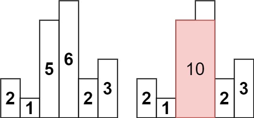
Input: heights = [2,1,5,6,2,3] Output: 10 Explanation: The above is a histogram where width of each bar is 1. The largest rectangle is shown in the red area, which has an area = 10 units.
Example 2:
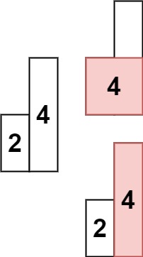
Input: heights = [2,4] Output: 4
Constraints:
1 <heights.length <= 10=50 <heights[i] <= 10=4
Here’s the GPT Guidance, we shall attempt this at another time again.
Absolutely! Let’s walk through the **Largest Rectangle in Histogram** problem step by step, focusing on **intuition and guided discovery**—not just the answer. ## Step 1: **What’s the Problem Asking?** Given a list of bar heights (each width 1), you want the area of the **largest rectangle** you can form by choosing one or more contiguous bars. - Each rectangle must be made up of consecutive bars. - The height of the rectangle is the **shortest bar** in that group. ## Step 2: **Brute Force Intuition** Suppose you want to try all possible rectangles: - For each bar, expand left and right as far as you can go without hitting a bar shorter than the current one. - For each bar, calculate the area: │ `area = height[i] * (right - left + 1)` │ **Why is this too slow?** For each bar, you might scan the whole array left and right: O(n²). ## Step 3: **Can You Do Better?** Let’s think: - For each bar, you want to know: **how far left and right can I expand before hitting a shorter bar?** - If you could, for every bar, **instantly** know the first shorter bar to the left and right, you could compute the area in O(1) for each bar. ## Step 4: **How Can We Find the First Shorter Bar to the Left and Right Efficiently?** This is where a **monotonic stack** comes in! - Imagine sweeping from left to right. - Keep a stack of indices of bars in **increasing height**. - When you see a bar that is **shorter** than the bar at the top of the stack, you know: │ - The bar at the top of the stack can’t extend any further right. │ - The current index is the "right boundary" for that bar. │ - The "left boundary" is the bar below it in the stack. │ ## Step 5: **Let’s Simulate a Small Example** Suppose `heights = `. - Start with an empty stack. - For each bar: │ - While the stack is not empty and the current bar is **shorter** than the bar at the top of the stack: │ │ - Pop the stack, calculate the area for that bar using the current index as the right boundary. │ │ - The left boundary is the new top of the stack (or -1 if the stack is empty). │ - Push the current index onto the stack. │ ## Step 6: **What About Bars Left in the Stack at the End?** - After you finish the array, bars left in the stack never found a shorter bar to their right. - For these, the right boundary is the end of the array. ## Step 7: **Ready to Try Coding?** Here’s a **framework** to help you get started: ```python def largestRectangleArea(heights): │ stack = [] # stores indices │ max_area = 0 │ n = len(heights) │ for i in range(n + 1): # +1 to handle the end │ │ curr_height = heights[i] if i < n else 0 # Sentinel: pop all at the end │ │ while stack and curr_height < heights[stack[-1]]: │ │ │ h = heights[stack.pop()] │ │ │ # width is from the previous index in stack + 1 to i - 1 │ │ │ w = i if not stack else i - stack[-1] - 1 │ │ │ max_area = max(max_area, h * w) │ │ stack.append(i) │ return max_area ``` ## Step 8: **Try Walking Through This On Paper** - Pick a small input, draw the stack, and see how the left/right boundaries are determined. - Notice how the stack helps you "remember" where each rectangle could start. ## Step 9: **Key Takeaways** - The stack is used to **remember indices of bars that haven't found a right boundary yet**. - When a shorter bar comes, you resolve all taller bars before it. - This approach is **O(n)** time and **O(n)** space. ## Want More Guidance? If you want to try implementing it yourself, start with the above framework and add print statements to see how the stack evolves. If you get stuck, let me know where, and I can nudge you further! **Ready to try it out? Or want a step-by-step trace with a specific input?**
※ 2.4.8.1. Constraints and Edge Cases
- constraints are large in space so it can’t be a slow approach like in the combinations one
※ 2.4.8.2. My Solution (Code)
※ 2.4.8.2.1. v1: Optimal Monotonic Stack solution
This code was guided by the bot, I couldn’t actually do this question.
1: class Solution: 2: │ def largestRectangleArea(self, heights: List[int]) -> int: 3: │ │ # we store indices and make decisions on the bars in this stack 4: │ │ stack = [] 5: │ │ max_area = 0 6: │ │ for i in range(len(heights) + 1): # ensures that the last bar is added to the stack 7: │ │ │ curr_height = heights[i] if i < len(heights) else 0 # Sentinel bar: pops all at the end 8: │ │ │ # the bar in consideration is always the bar at the top of the stack 9: │ │ │ while (found_right_boundary:= stack and curr_height < heights[stack[-1]]): 10: │ │ │ min_height = heights[stack.pop()] 11: │ │ │ # empty stack: either i = 0 or the inputs are such that it's a consistently declining slope so far 12: │ │ │ width = i if not stack else i - stack[-1] - 1 13: │ │ │ max_area = max(max_area, min_height * width) 14: │ │ │ 15: │ │ │ # add the small left boundary 16: │ │ │ stack.append(i) 17: │ │ │ 18: │ │ return max_area
Here’s an alternative approach. This avoids the need for the sentinel bar by adding a sentinel value within the stack.
1: class Solution: 2: │ def largestRectangleArea(self, heights: List[int]) -> int: 3: │ │ stack = [-1] 4: │ │ max_area = 0 5: │ │ for i, h in enumerate(heights): 6: │ │ │ while stack[-1] != -1 and heights[stack[-1]] >= h: 7: │ │ │ │ height = heights[stack.pop()] 8: │ │ │ │ width = i - stack[-1] - 1 9: │ │ │ │ max_area = max(max_area, height * width) 10: │ │ │ stack.append(i) 11: │ │ n = len(heights) 12: │ │ while stack[-1] != -1: 13: │ │ │ height = heights[stack.pop()] 14: │ │ │ width = n - stack[-1] - 1 15: │ │ │ max_area = max(max_area, height * width) 16: │ │ return max_area
Both these solutions have the following complexity:
for n number of bars:
- time: \(O(n)\) for iterating through the array and the monotonic stack
- space: \(O(n)\) for creating a monotonic stack
※ 2.4.8.2.2. v2: 2-pass linear-time solution
This is more explicit and easier to reason with.
The asymptotic complexity is the same as the previous one but this is expected to be slower because it’s a 2-pass solution while the monotonic stack version is a 1-pass solution.
1: class Solution: 2: │ def largestRectangleArea(self, heights: List[int]) -> int: 3: │ │ n = len(heights) 4: │ │ left = [-1] * n 5: │ │ right = [n] * n 6: │ │ stack = [] 7: │ │ 8: │ │ # Compute left boundaries 9: │ │ for i in range(n): 10: │ │ │ while stack and heights[stack[-1]] >= heights[i]: 11: │ │ │ │ stack.pop() 12: │ │ │ left[i] = stack[-1] if stack else -1 13: │ │ │ stack.append(i) 14: │ │ │ 15: │ │ stack.clear() 16: │ │ 17: │ │ # Compute right boundaries 18: │ │ for i in range(n - 1, -1, -1): 19: │ │ │ while stack and heights[stack[-1]] >= heights[i]: 20: │ │ │ │ stack.pop() 21: │ │ │ right[i] = stack[-1] if stack else n 22: │ │ │ stack.append(i) 23: │ │ │ 24: │ │ # Calculate max area 25: │ │ max_area = 0 26: │ │ for i in range(n): 27: │ │ │ width = right[i] - left[i] - 1 28: │ │ │ area = heights[i] * width 29: │ │ │ max_area = max(max_area, area) 30: │ │ return max_area
Explanation
- Left Boundaries: For each bar, find the index of the first bar to the left that is shorter. If none, use -1.
- Right Boundaries: For each bar, find the index of the first bar to the right that is shorter. If none, use n.
- Area Calculation: For each bar, the width is right[i] - left[i] - 1, and the area is heights[i] * width.
※ 2.4.8.3. My Approach/Explanation
- Initial thinking:
- I just need to accumulate the max so it’s like sweep
- the areas need to be contiguous, so this is not really like the rainwater trapping problem
- I think I need to collapse both the dimensions: height and width
- At the same time I know that there’s
- I also know that I can’t ignore / clear the stack if a bigger one is found because if the
nis large, then I could group together a bunch ofns (not sure if this judgement is accurate)
※ 2.4.8.4. My Learnings/Questions
- Tackle the brute force version first then look at how to optimise. The essence of the problem is what we need to identify.
- Intuition:
- To explore the primitives behind the question, it’s important to think about HOW the brute force approach is done. Then, the question boils down to how to add efficiencies to improve on the brute force approach. In this case, the brute force: for each bar, go as far left and right possible until a boundary is reached. A boundary is one where the next candidate is smaller than current bar in consideration. This helps to find the width and then the height is just current bar’s height.
- So it’s the boundary-finding that needs to be optimised. So we need to think of what data-structure we can use for this:
- if we sweep through things, we can keep looking for right boundaries (when new candidate is smaller than existing known ones).
- so we just need to store the (the index of) currently-accumulating candidates. They naturally will be increasing in height, so it’s a monotonically increasing stack (stack because we need to keep a history of the candidates that are being accumulated).
- so at any time, as we sweep left to right on the original heights:
- we are accumulating for the current element at the TOP of the stack
- we find that bar’s right boundary once we come across a candidate that is SMALLER than current top of stack.
- BECAUSE we are keeping a monotonically increasing stack, the element just below the top of the stack is the LEFT BOUNDARY of the current element at the top of the stack
- now that we have the 2 boundaries, the height would be the height of the bar that the current top of the stack is pointing to, we can compare with the max-accumulation variable that we use.
- Careful about:
- the iteration range is
len(arr) + 1. Our bars are being inserted into the stack, we need to insert the right-most bar as well. That’s why we need go “out of bounds” - Sentinel Values: because of the iteration range, the height calculation for
curr_heightatidx = (len(heights) -1 )has to use a0sentinel-value.- question: elaborate more on the mental model behind the term “sentinel value”, when it should be used and such
- width calculation:
- the stack will only be empty if there’s no left boundary (first elem or the inputs are like that [a consistent declining slop]), in which case we just keep it at
i - else, it’s
(right_boundary - left_boundary) - 1because width of the right boundary isn’t considered.
- the stack will only be empty if there’s no left boundary (first elem or the inputs are like that [a consistent declining slop]), in which case we just keep it at
- the iteration range is
General Intuition on Monotonic stack pattern. It seems that usually, the in-consideration elements are the ones that we’re putting in the stack. They’re in there because we need to preserve some intermediate order of these in-consideration elements.
- in this case, we’re putting the unresolved elements in the monotonic stack.
- this is also useful when we want to keep a history of considerations while we find boundaries for things. The history point rings true here.
Show/Hide Md CodeYour intuition is exactly right, and it’s echoed in the literature on monotonic stacks: - **The stack holds "unresolved" elements**—those for which you haven’t yet found the next smaller (or greater) element. - **History preservation:** The stack acts as a memory of the indices (or values) of elements that are still "waiting" for their boundary to be found. As you process each new element, you check if it resolves the boundary for any of the elements in the stack[1][2][3]. ### Why keep unresolved elements in the stack? - **Boundary finding:** For problems like "next smaller/greater element," you need to know, for each element, when a boundary (i.e., a smaller/greater bar) is encountered. You can't know this until you see a bar that breaks the monotonic property. - **Efficient processing:** By keeping a stack of unresolved elements, you process each element only when its boundary is found, ensuring O(n) time[1][2][3]. - **Order preservation:** The stack maintains a partial order (monotonically increasing or decreasing), which is crucial for efficiently determining boundaries. ### Example: Largest Rectangle in Histogram - As you sweep through the histogram, each bar is pushed onto the stack if it hasn't yet found a right boundary (a bar shorter than itself). - When you find a shorter bar, you pop from the stack, resolving the right boundary for the popped bar. The element below in the stack is the left boundary. - The stack thus "remembers" all the bars for which you haven't yet found a right boundary. > “Monotonic stacks are ideal for problems where you need to find the ‘next’ element based on specific criteria, like the next greater element. They are also effective for dynamically maintaining the maximum or minimum element in a changing window. ... By dynamically removing irrelevant elements and preserving a monotonic order, they enable efficient solutions to problems that might otherwise be much slower.”[2] ### General Principle - **The stack is a history of candidates**: It holds all elements still waiting for their answer (boundary), and as soon as the answer is found, they're popped and processed. - **This pattern is powerful** for a wide range of problems involving "next" or "previous" constraints (e.g., next greater/smaller, sliding window maximum/minimum)[1][2][3]. **References:** [1] algo.monster: Monotonic Stack/Queue Intro [2] teddysmith.io: Simplify Algorithm Design with the Monotonic Stack Pattern [3] GeeksforGeeks: Introduction to Monotonic Stack [1] https://algo.monster/problems/mono_stack_intro [2] https://teddysmith.io/monotonic-stack-algorithm-pattern/ [3] https://www.geeksforgeeks.org/dsa/introduction-to-monotonic-stack-2/ [4] https://en.wikipedia.org/wiki/Sorting_algorithm [5] https://stackoverflow.com/questions/72625101/how-do-i-solve-it-with-a-monotonic-stack [6] https://labuladong.online/algo/en/data-structure/monotonic-stack/ [7] https://en.wikipedia.org/wiki/Monotonic_function [8] https://liuzhenglaichn.gitbook.io/algorithm/monotonic-stack [9] https://blog.devgenius.io/monotonic-stack-algorithm-pattern-7bfac59157c2?gi=5dccec2461a5 [10] https://stackoverflow.com/questions/77878403/finding-all-sequences-with-same-stack-operations-to-make-monotonic-stack-from-th
※ 2.4.9. [Depth Blind 1] Remove Duplicate Letters (316) failed greedy monotonic_stack
Given a string s, remove duplicate letters so that every letter
appears once and only once. You must make sure your result is the
smallest in lexicographical order among all possible results.
Example 1:
Input: s = "bcabc" Output: "abc"
Example 2:
Input: s = "cbacdcbc" Output: "acdb"
Constraints:
1 <s.length <= 10=4sconsists of lowercase English letters.
Note: This question is the same as 1081: https://leetcode.com/problems/smallest-subsequence-of-distinct-characters/
※ 2.4.9.1. Constraints and Edge Cases
Nothing fancy
※ 2.4.9.2. My Solution (Code)
※ 2.4.9.2.1. v1: guided
1: from collections import Counter 2: 3: class Solution: 4: │ def removeDuplicateLetters(self, s: str) -> str: 5: │ │ # keeps the last position of a duplicate, if found 6: │ │ last_pos = {} 7: │ │ for idx, char in reversed(list(enumerate(s))): 8: │ │ │ if char not in last_pos: 9: │ │ │ │ last_pos[char] = idx 10: │ │ │ │ 11: │ │ stack = [] # use this to build the res 12: │ │ visited = set() 13: │ │ for idx, c in enumerate(s): 14: │ │ │ if not stack: 15: │ │ │ │ stack.append(c) 16: │ │ │ │ visited.add(c) 17: │ │ │ │ continue 18: │ │ │ │ 19: │ │ │ if c in visited: 20: │ │ │ │ continue 21: │ │ │ │ 22: │ │ │ # as long as top of stack can be discarded: 23: │ │ │ # A: it is lexically bigger than C AND 24: │ │ │ # B: it comes later 25: │ │ │ while(stack and stack[-1] > c and idx < last_pos[stack[-1]]): 26: │ │ │ │ visited.remove(stack.pop()) 27: │ │ │ │ 28: │ │ │ stack.append(c) 29: │ │ │ visited.add(c) 30: │ │ │ 31: │ │ return "".join(stack)
- build string such that it contains unique letters
- string is lexicographically the smallest
- so we need to make decisions on whether or not to discard a letter.
- result must be in order, and is the smallest possible
If we know that we can make a better decision in the future than now, then we greedily remove that from our current decisions.
- for each letter, we need to know the last occurrence of each letter in s. This tells us if the character appears again later in the string
- we will use our stack to build the final string.
- for each c in s:
- case 1: c has been encountered before and we have it in the stack
- case 2: c is new
- while top of stack is lexicographically greater than c and top char appears again in s (i.e. can be placed later), then that top of stack char can be discarded
- pop that top of stack
- push c to the top of the stack
- join chars in c.
※ 2.4.9.3. My Approach/Explanation
The final solution hinges on the core intuition that “can we make a better choice in the future?”. If so, then we remove the current choices made
※ 2.4.9.4. My Learnings/Questions
- Remember that stack is also just a list so we can read it bottom to top just like that.
Key intuition:
If we know that we can make a better decision in the future than now, then we greedily remove that from our current decisions.
※ 2.4.9.5. Prompt for GPT Evaluation
Please do the following:
- Evaluate the correctness of my solution. Are there any logical or edge case errors?
- Analyze the time and space complexity of my code.
- Suggest improvements in code style, efficiency, or clarity.
- Compare my approach to the optimal solution (if different).
- Provide a sample optimal solution (if mine is not optimal).
- Point out any Pythonic (or language-specific) improvements.
Are there any completely different approaches to this problem?
- e.g something that uses a completely different data structure
If so, then help me gain the intuition for it and show the code clearly
- Answer my specific questions (if any are listed above).
※ 2.4.9.6. Prompt for GPT Evaluation (with Greedy)
Please do the following:
- Evaluate the correctness of my solution. Are there any logical or edge case errors?
- Analyze the time and space complexity of my code.
- Suggest improvements in code style, efficiency, or clarity.
- Compare my approach to the optimal solution (if different).
- Provide a sample optimal solution (if mine is not optimal).
- Point out any Pythonic (or language-specific) improvements.
Are there any completely different approaches to this problem?
- e.g something that uses a completely different data structure
If so, then help me gain the intuition for it and show the code clearly
- Answer my specific questions (if any are listed above).
ALso help me evaluate this in the context of greedy algorithms, ensuring that a good framework of presenting this problem into a greedy algo is given / understood.
※ 2.4.9.7. Prompt for GPT Evaluation (with DP)
Please do the following:
- Evaluate the correctness of my solution. Are there any logical or edge case errors?
- Analyze the time and space complexity of my code.
- Suggest improvements in code style, efficiency, or clarity.
- Compare my approach to the optimal solution (if different).
- Provide a sample optimal solution (if mine is not optimal).
- Point out any Pythonic (or language-specific) improvements.
Are there any completely different approaches to this problem?
- e.g something that uses a completely different data structure
If so, then help me gain the intuition for it and show the code clearly
- Answer my specific questions (if any are listed above).
ALso help me evaluate this in the context of greedy algorithms, ensuring that a good framework of presenting this problem into a greedy algo is given / understood.
Additionally, use my notes for Dynamic Programming and use the recipes that are here.
Recipe to define a solution via DP
[Generate Naive Recursive Algo]
Characterise the structure of an optimal solution \(\implies\) what are the subproblems? \(\implies\) are they independent subproblems? \(\implies\) how many subproblems will there be?
- Recursively define the value of an optimal solution \(\implies\) does this have the overlapping sub-problems property? \(\implies\) what’s the cost of making a choice? \(\implies\) how many ways can I make that choice?
- Compute value of an optimal solution
- Construct optimal solution from computed information Defining things
- Optimal Substructure:
A problem exhibits “optimal substructure” if an optimal solution to the problem contains within it optimal solutions to subproblems.
Elements of Dynamic Programming: Key Indicators of Applicability [1] Optimal Sub-Structure Defining “Optimal Substructure” A problem exhibits optimal substructure if an optimal solution to the problem contains within it optimal solutions to sub-problems.
- typically a signal that DP (or Greedy Approaches) will apply here.
- this is something to discover about the problem domain Common Pattern when Discovering Optimal Substructure
solution involves making a choice e.g. choosing an initial cut in the rod or choosing what k should be for splitting the matrix chain up
\(\implies\) making the choice also determines the number of sub-problems that the problem is reduced to
- Assume that the optimal choice can be determined, ignore how first.
- Given the optimal choice, determine what the sub-problems looks like \(\implies\) i.e. characterise the space of the subproblems
- keep the space as simple as possible then expand
typically the substructures vary across problem domains in 2 ways:
[number of subproblems]
how many sub-problems does an optimal solution to the original problem use?
- rod cutting:
# of subproblems = 1(of size n-i) where i is the chosen first cut lengthmatrix split:
# of subproblems = 2(left split and right split)[number of subproblem choices]
how many choices are there when determining which subproblems(s) to use in an optimal solution. i.e. now that we know what to choose, how many ways are there to make that choice?
- rod cutting: # of choices for i = length of first cut,
nchoices- matrix split: # of choices for where to split (idx k) =
j - iNaturally, this is how we analyse the runtime:
# of subproblems * # of choices @ each sub-problem- Reason to yourself if and how solving the subproblems that are used in an optimal solution means that the subproblem-solutions are also optimal. This is typically done via the
cut-and-paste argument.Caveat: Subproblems must be
independent
- “independent subproblems”
- solution to one subproblem doesn’t affect the solution to another subproblem for the same problem
example: Unweighted Shortest Path (independent subproblems) vs Unweighted Longest Simple Path (dependent subproblems)
Consider graph \(G = (V,E)\) with vertices \(u,v \notin V\)
- Unweighted shortest path: we want to find path \(u\overset{p}{\leadsto}v\) then we can break it down into subpaths \(u\overset{p1}{\leadsto}w\overset{p2}{\leadsto}v\) (optimal substructure). If path, p, is optimal from \(u\leadsto{v}\) then p1 must be shortest path from \(u\leadsto{w}\) and likewise p2 must be shortest path from \(w\leadsto{v}\) (cut-and-paste argument) Here, we know that the subproblems are independent.
- Unweighted Longest Simple Path: the subproblems can have paths that overlap (not subproblem overlap), hence it’s not independent because the vertices that appear can appear in the solution to the second subproblem
Terminology: Optimal substruture vs optimal solution optimal substructure is a property that enables efficient computation of the optimal value, while the solution is the specific configuration that yields that optimal value
You’re right that in dynamic programming algorithms for optimization problems, the goal is usually to find an optimal solution rather than the unique optimal solution. Here’s how the optimal substructure and the actual solution differ:
### Optimal Substructure
The optimal substructure refers to the property that the optimal solution to a problem can be constructed from the optimal solutions to its subproblems. This means that if we know the optimal solutions to the subproblems, we can efficiently determine the optimal solution to the overall problem.
For example, in the rod cutting problem, if we know the maximum revenue for rods of length 1 to n-1, we can efficiently determine the maximum revenue for a rod of length n by considering cutting the rod at each possible length and taking the maximum revenue.
### The Solution
The actual solution, on the other hand, refers to the specific configuration or set of choices that yields the optimal value. In the rod cutting problem, the solution would be the specific way to cut the rod that results in the maximum revenue.
The key difference is that the optimal substructure allows us to efficiently compute the optimal value, but it doesn’t necessarily specify the exact solution. There may be multiple solutions that yield the same optimal value.
For example, in the rod cutting problem, there may be multiple ways to cut the rod that result in the same maximum revenue. The optimal substructure allows us to efficiently compute the maximum revenue, but it doesn’t specify which particular cutting configuration to choose.
So in summary, the optimal substructure is a property that enables efficient computation of the optimal value, while the solution is the specific configuration that yields that optimal value. Dynamic programming algorithms leverage the optimal substructure to efficiently compute the optimal value, but the actual solution may not be uniquely determined.
Citations: [1] https://library.fiveable.me/key-terms/programming-for-mathematical-applications/optimal-substructure [2] https://afteracademy.com/blog/optimal-substructure-and-overlapping-subproblems/ [3] https://www.geeksforgeeks.org/optimal-substructure-property-in-dynamic-programming-dp-2/ [4] https://labuladong.gitbook.io/algo-en/i.-dynamic-programming/optimalsubstructure [5] https://stackoverflow.com/questions/33563230/optimal-substructure-in-dynamic-programing [6] https://en.wikipedia.org/wiki/Optimal_substructure [7] https://www.cs.cmu.edu/~15451-f22/lectures/lec09-dp1.pdf [8] https://www.javatpoint.com/optimal-substructure-property
[2] Overlapping Sub-Problems
- DP should be disambiguated from Divide & Conquer:
- for Divide&Conquer, choosing a division point generates brand new problems that likely don’t overlap
- for DP, the space of sub-problems is small and hence if done purely recursively, the same operations get computed multiple times
[Practical point] Reconstructing an optimal solution Since one way to look at DP is table-filling, we typically have:
- table of costs
- table of optimal choices
the table of optimal choices can be built from the table of costs, but we want to avoid recalculating the optimal choices
Memoisation as an alternative
- the textbook used sees this as an alternative and memoised tables as the aux DS for recursive, top-down approaches
- memoisation also exploits the observation that the space of the subproblems is small and hence overlapping
Common Misconceptions Here are some common misconception, based on what perplexity says
Based on the search results, here are some of the common misconceptions that learners have about dynamic programming:
## 1. Misconceptions about the Definition and Purpose of Dynamic Programming
- Thinking that recursion and dynamic programming are explicitly different concepts[3].
- Believing that dynamic programming is exclusively used to solve optimization problems[3].
## 2. Misconceptions about the Optimal Substructure Property
- Assuming that the optimal solution to a problem can be constructed from any combination of optimal solutions to its subproblems, rather than specific optimal solutions to the right subproblems[1][2].
- Thinking that the optimal solution to a problem can be constructed from optimal solutions to unrelated subproblems[4].
## 3. Misconceptions about Memoization and Tabulation
- Failing to recognize that memoization (top-down) and tabulation (bottom-up) are two different implementation strategies for dynamic programming[1][2].
- Believing that memoization always involves recursion and tabulation always involves iteration[1][2].
## 4. Misconceptions about the Filling Order of the DP Table
- Assuming that the DP table must always be filled in a specific order (e.g., always from small to big cases), without understanding that the order depends on the problem’s dependencies and constraints[1][2][4].
## 5. Misconceptions about the Relationship between Subproblems
- Thinking that the solutions to all subproblems are needed to solve the original problem, rather than understanding that only specific optimal solutions to the right subproblems are needed[1][2].
## 6. Misconceptions about the Efficiency of Dynamic Programming
- Believing that dynamic programming always leads to polynomial-time algorithms, without understanding that it can sometimes only slightly improve the exponential-time complexity[4].
Understanding and addressing these common misconceptions can help learners develop a more accurate and comprehensive understanding of dynamic programming and its applications.
Citations: [1] https://dl.acm.org/doi/10.1145/3159450.3159528 [2] https://dl.acm.org/doi/abs/10.1145/3159450.3159528 [3] https://ics.uci.edu/~mikes/papers/Student_Misconceptions_Dynamic_Programming.pdf [4] https://www.cs.cmu.edu/~15451-f22/lectures/lec09-dp1.pdf [5] https://www.reddit.com/r/compsci/comments/er05hn/help_me_wrap_my_head_around_dynamic_programming/ [6] https://yourbasic.org/algorithms/dynamic-programming-explained/ [7] https://stackoverflow.com/questions/33563230/optimal-substructure-in-dynamic-programing [8] https://lec.inf.ethz.ch/DA/2020/slides/daLecture13.en.pdf
Greedy Algos vs DP When comparing greedy strategies and dynamic programming (DP), it’s essential to understand how they differ in methodology, application, and the nature of the problems they solve. Both approaches involve identifying optimal substructures, but they apply this concept in distinct ways. Here’s a detailed disambiguation based on the search results:
### 1. Definition and Approach
- Greedy Strategy:
- A greedy algorithm makes the most optimal choice at each step with the hope that these local optimum choices will lead to a global optimum solution. It does not consider the overall impact of the current choice on future decisions.
- Greedy algorithms are typically simpler and faster to implement, as they do not require storing results of subproblems. However, they do not guarantee an optimal solution for all problems.
- Dynamic Programming:
- Dynamic programming is a technique used to solve complex problems by breaking them down into simpler subproblems. It is based on the principles of optimal substructure and overlapping subproblems.
- DP guarantees an optimal solution by considering all possible cases and storing the results of subproblems to avoid redundant computations. This can lead to higher time and space complexity compared to greedy algorithms.
### 2. Optimal Substructure
- Greedy Algorithms:
- Greedy algorithms rely on the greedy choice property, which means that a locally optimal choice leads to a globally optimal solution. However, this property does not hold for all problems, which is why greedy algorithms may fail to find the optimal solution in some cases.
- Dynamic Programming:
- Dynamic programming explicitly uses the optimal substructure property, where an optimal solution to a problem can be constructed from optimal solutions of its subproblems. DP ensures that all relevant subproblems are considered, leading to a guaranteed optimal solution.
### 3. Subproblem Reuse
- Greedy Strategy:
- Greedy algorithms typically do not reuse solutions to subproblems. Each decision is made independently based on the current state without revisiting previous choices.
- Dynamic Programming:
- DP explicitly solves and caches solutions to overlapping subproblems. This reuse of subproblem solutions is a key feature of dynamic programming, allowing for efficient computation.
### 4. Complexity and Efficiency
- Greedy Algorithms:
- Greedy algorithms are generally more efficient in terms of time complexity due to their straightforward approach. They often run in linear or logarithmic time, depending on the problem.
- They are suitable for problems where local optimization leads to global optimization, such as in minimum spanning trees or certain shortest path problems.
- Dynamic Programming:
- DP can be less efficient than greedy algorithms in terms of time complexity, especially if every possible solution is computed. However, proper use of memoization can mitigate this.
- DP is applicable to problems with overlapping subproblems and optimal substructure, such as the Fibonacci sequence, longest common subsequence, or knapsack problems.
### 5. Examples
- Greedy Algorithms:
- Common examples include:
- Fractional Knapsack Problem: Where you can take fractions of items.
- Minimum Spanning Tree: Algorithms like Prim’s and Kruskal’s.
- Huffman Coding: For optimal prefix codes.
- Dynamic Programming:
- Common examples include:
- 0/1 Knapsack Problem: Where you cannot take fractions of items.
- Longest Common Subsequence: Finding the longest subsequence present in both sequences.
- Matrix Chain Multiplication: Finding the most efficient way to multiply a given sequence of matrices.
### Conclusion
In summary, while both greedy strategies and dynamic programming involve the concept of optimal substructure, they differ significantly in their approach to problem-solving. Greedy algorithms make decisions based on local optimality without revisiting previous choices, whereas dynamic programming systematically considers all possible subproblems and their solutions to ensure a globally optimal result. Understanding these differences allows for better problem-solving strategies and the appropriate application of each method based on the problem’s characteristics.
Citations: [1] https://www.boardinfinity.com/blog/greedy-vs-dp/ [2] https://www.shiksha.com/online-courses/articles/difference-between-greedy-and-dynamic-programming-blogId-158053 [3] https://www.interviewbit.com/blog/difference-between-greedy-and-dynamic-programming/ [4] https://stackoverflow.com/questions/16690249/what-is-the-difference-between-dynamic-programming-and-greedy-approach [5] https://www.geeksforgeeks.org/greedy-approach-vs-dynamic-programming/ [6] https://byjus.com/gate/difference-between-greedy-approach-and-dynamic-programming/ [7] https://www.cs.cmu.edu/~15451-f22/lectures/lec09-dp1.pdf [8] https://ics.uci.edu/~mikes/papers/Student_Misconceptions_Dynamic_Programming.pdf
General Takeaways Bottom-up vs Top-Down
- we can use a subproblem graph to show the relationship with the subproblems ==> diff b/w bottom up and top-down is how these deps are handled (recursive-called or soundly iterated with a proper direction)
- aysymptotic runtime is pretty similar since both solve similar \(\Omega(n^{2})\)
- Bottom up:
- basically considers order at which the subproblems are solved
- because of the ordered way of solving the smaller sub-problems first, there’s no need for recursive calls and code can be iterative entirely
- so no overhead from function calls
- no chance of stack overflow
- benefits from data-locality
- a way to see the vertices of the subproblem graph such that the subproblems y-adjacent to a given subproblem x is solved before subproblem x is solved
※ 2.4.9.8. [Optional] Additional Context
Honestly, not being able to catch this is demoralising. However what gives hope is that this isn’t as bad if we consider that the key intuition (we can discard the choice if we know that there’s a better one in the future) is there.
※ 2.4.10. [Depth-Blind 2] 132 Pattern (456) failed subsequence stack
Given an array of n integers nums, a 132 pattern is a subsequence
of three integers nums[i], nums[j] and nums[k] such that
i < j < k and nums[i] < nums[k] < nums[j].
Return true if there is a 132 pattern in =nums=/, otherwise,
return/ =false=/./
Example 1:
Input: nums = [1,2,3,4] Output: false Explanation: There is no 132 pattern in the sequence.
Example 2:
Input: nums = [3,1,4,2] Output: true Explanation: There is a 132 pattern in the sequence: [1, 4, 2].
Example 3:
Input: nums = [-1,3,2,0] Output: true Explanation: There are three 132 patterns in the sequence: [-1, 3, 2], [-1, 3, 0] and [-1, 2, 0].
Constraints:
n =nums.length=1 <n <= 2 * 10=5-10=^{=9}= <= nums[i] <= 10=9
※ 2.4.10.1. Constraints and Edge Cases
<list constraints, input limits, or tricky edge cases here>
※ 2.4.10.2. My Solution (Code)
※ 2.4.10.2.1. v0: wrong, partial test cases
1: class Solution: 2: │ def find132pattern(self, nums: List[int]) -> bool: 3: │ │ # we only keep an increasing stack (so top of the stack is highest) always 4: │ │ stack = [] 5: │ │ for num in nums: 6: │ │ │ # case 1: if insuficient 7: │ │ │ while stack and num < (top:=stack[-1]) and len(stack) < 2: 8: │ │ │ │ stack.pop() 9: │ │ │ │ 10: │ │ │ if len(stack) >= 2 and stack[-1] > num and stack[-2] < num: 11: │ │ │ │ return True 12: │ │ │ │ 13: │ │ │ # if len(stack) >= 2 and num < (top:=stack[-1]): 14: │ │ │ # return True 15: │ │ │ 16: │ │ │ stack.append(num) 17: │ │ │ 18: │ │ │ 19: │ │ return False
※ 2.4.10.2.2. v1: guided optimal
1: class Solution: 2: │ def find132pattern(self, nums: List[int]) -> bool: 3: │ │ n = len(nums) 4: │ │ if n < 3: 5: │ │ │ return False 6: │ │ │ 7: │ │ min_left = [float('inf')] * n 8: │ │ curr_min = nums[0] 9: │ │ for i in range(len(nums)): 10: │ │ │ curr_min = min(curr_min, nums[i]) 11: │ │ │ min_left[i] = curr_min 12: │ │ │ 13: │ │ stack = [] # stores possible 2 values: 14: │ │ for j in range(n - 1, -1, -1): 15: │ │ │ while stack and stack[-1] <= min_left[j]: 16: │ │ │ │ stack.pop() 17: │ │ │ │ 18: │ │ │ # now all in the stack are worthy of being k 19: │ │ │ if stack and stack[-1] < nums[j]: 20: │ │ │ │ return True 21: │ │ │ else: # now we can consider j as a 22: │ │ │ │ stack.append(nums[j]) 23: │ │ │ │ 24: │ │ return False
See explanation below:
※ 2.4.10.3. My Approach/Explanation
※ 2.4.10.3.1. Reframing the Subsequence
We want 3 indices, left to right such that we get: smallest, peak, drop
drop can’t be smaller than smallest either.
At index, j, can we find a “1” somewhere left (for nums[i]) and a “2” somewhere to its right that is less than current but more than min?
※ 2.4.10.3.2. Consider brute force
It’s just picking every possible triplet, (i,j,k) which would happen in \(O(n^{3})\) and so it’s too slow and we have to prune it.
※ 2.4.10.3.3. Optimising: fixing the middle (j) (peak)
If we can fix the peak then at each j, we could:
- try to know the smallest element to its left (
min_leftfor i < j) - try to find a 2 to its right so that \(min_{i} < nums[k] < nums[j]\)
How do we do this?
we could technically precompute \(min_{i}\).
for “2” values, we want to quickly be able to check if there’s any right-side value in the interval \(min_{i} < nums[k] < nums[j]\) as we go from right to left.
※ 2.4.10.3.4. How to use a stack here
Use the stack for finding “2”s. As we go from right to left:
for each nums[j]:
case A: pop off elements in stack that are less than left_min[j] because they can’t be “2”
case B: found 132: if stack top < nums[j] and stack top > left_min[j])
case C: nums[j] should be considered as a “2” value
※ 2.4.10.4. My Learnings/Questions
- Lmao my brain is fried.
※ 2.4.10.5. [Optional] Additional Context
I think I’m super tired.
But then again, I think I don’t have a good intuition on stack problems in general.
※ 2.5. Binary Search
| Headline | Time | ||
|---|---|---|---|
| Total time | 2:05 | ||
| Binary Search | 2:05 | ||
| [22] Binary Search (704) | 0:07 | ||
| [23] Search a 2D Matrix (74) | 0:10 | ||
| [24] Koko Eating Bananas (875) | 0:50 | ||
| [25] Find Minimum in Rotated Sorted… | 0:30 | ||
| [26] Time Based Key Value Store (981) | 0:28 |
※ 2.5.2. [22] Binary Search (704)
Given an array of integers nums which is sorted in ascending order,
and an integer target, write a function to search target in nums.
If target exists, then return its index. Otherwise, return -1.
You must write an algorithm with O(log n) runtime complexity.
Example 1:
Input: nums = [-1,0,3,5,9,12], target = 9 Output: 4 Explanation: 9 exists in nums and its index is 4
Example 2:
Input: nums = [-1,0,3,5,9,12], target = 2 Output: -1 Explanation: 2 does not exist in nums so return -1
Constraints:
1 <nums.length <= 10=4-10=^{=4}= < nums[i], target < 10=4- All the integers in
numsare unique. numsis sorted in ascending order.
※ 2.5.2.1. Constraints and Edge Cases
The common edge cases to consider for binary search kind of questions:
- Empty array: All approaches return -1.
- Single element: All approaches work.
- Target not present: All approaches return -1.
- Target at first/last position: All approaches find it correctly.
※ 2.5.2.2. My Solution (Code)
Here’s the solution, it’s great already. It uses a recursive helper.
1: class Solution: 2: │ def search(self, nums: List[int], target: int) -> int: 3: │ │ def helper(left, right): 4: │ │ │ if (left >= right): 5: │ │ │ │ return -1 6: │ │ │ │ 7: │ │ │ # needs to account for the left being an offset and not zero-ed 8: │ │ │ mid_idx = left + ((right - left) // 2) 9: │ │ │ mid = nums[mid_idx] 10: │ │ │ if target == mid: 11: │ │ │ │ return mid_idx 12: │ │ │ elif target < mid: 13: │ │ │ │ return helper(left, mid_idx) 14: │ │ │ else: 15: │ │ │ │ return helper(mid_idx + 1, right) 16: │ │ │ │ 17: │ │ return helper(0, len(nums))
Complexity Analysis:
- Time: \(O(logn)\) because of the half-half divisioning
- Space: \(O(logn)\) because of the stack frames created in the recursive process
for completeness, let’s look at the other implementations as well:
iterative while-looped I really dislike this because I don’t like while loops but because python doesn’t optimise for tail recursion, this is a better solution for longer inputs.
Show/Hide Python Code1: class Solution: 2: │ def search(self, nums: List[int], target: int) -> int: 3: │ │ left, right = 0, len(nums) - 1 4: │ │ while left <= right: 5: │ │ │ mid = left + (right - left) // 2 6: │ │ │ if nums[mid] == target: 7: │ │ │ │ return mid 8: │ │ │ elif nums[mid] < target: 9: │ │ │ │ left = mid + 1 10: │ │ │ else: 11: │ │ │ │ right = mid - 1 12: │ │ return -1
This has better space usage compared to the recursive approach because we don’t need to handle any stack frames in memory, pointer movements are all done in place and in \(O(1)\) space
Complexity Analysis:
- Time: \(O(logn)\) because of the half-half divisioning
- Space: \(O(1)\) no rescursion stack
using the
bisect_leftfunction from thebisectmoduleShow/Hide Python Code1: from bisect import bisect_left 2: 3: class Solution: 4: │ def search(self, nums: List[int], target: int) -> int: 5: │ │ idx = bisect_left(nums,target) 6: │ │ return idx if idx < len(nums) and nums[idx] == target else -1
Complexity Analysis:
- Time: \(O(logn)\) because of the half-half divisioning
- Space: \(O(1)\) (C implementation uses no extra stack)
※ 2.5.2.3. My Approach/Explanation
Simple binary search BECAUSE of the monotonically increasing array. That’s the key characteristic that allows us to do this.
Also, careful on the calculation of the mid index, it should use the offset of left boundary because not always will the left boundary be 0.
※ 2.5.2.4. My Learnings/Questions
- careful on the question requirements part: what should be returned (idx/value/bool?)
- careful when defining the mid idx because not always will
left = 0hence you need to add the offset:mid_idx = left + ( (right - left) // 2 ) - Alternatives:
- Hash Map:
- You could preprocess the array into a dictionary mapping values to indices.
- Time: O(1) lookup, but O(n) preprocessing and O(n) space.
- Not optimal for this problem, as binary search is faster for repeated queries on sorted arrays.
- Interpolation Search:
- For uniformly distributed data, interpolation search can be faster than binary search on average, but worst-case is still O(log n).
- Rarely used in practice unless the data distribution is known.
- Exponential Search:
- Useful if the array is unbounded or very large and you need to find the range first.
- Intuition for binary search:
- Binary search is optimal for sorted arrays due to the divide-and-conquer property. Other data structures (e.g., hash maps) are only better if you need O(1) lookup and don’t care about space or if the array isn’t sorted.
- the monotonically consistent order is what gives rise to the divide-and-conquer property
Also read this to understand Interpolation Search and Exponential Search methods:
Show/Hide Md Code### Interpolation Search **Interpolation search** is a search algorithm designed for **sorted arrays**, especially when the data is *uniformly distributed* (the difference between consecutive elements is roughly constant). Unlike binary search, which always checks the middle element, interpolation search estimates the likely position of the target based on its value relative to the values at the current search bounds. #### How it works: - It calculates a "probe" position using the formula: │ $$ │ \text{pos} = \text{low} + \frac{(x - \text{array[low]}) \times (\text{high} - \text{low})}{\text{array[high]} - \text{array[low]}} │ $$ │ where `x` is the target value, and `low`/`high` are the current search bounds. - If the value at `pos` matches the target, it returns the index. - If the value at `pos` is less than the target, it searches the right subarray; if greater, it searches the left subarray. - This process repeats until the target is found or the search space is empty[1][2][5][6]. **Performance:** - **Average case:** $$O(\log \log n)$$ comparisons for uniformly distributed data (faster than binary search). - **Worst case:** $$O(n)$$ comparisons (if the data is not uniformly distributed or is skewed)[2][4][5]. **Intuition:** It works like looking up a name in a phone book: you estimate where the name should be, rather than always opening to the middle[2][6][7]. ### Exponential Search **Exponential search** is useful when you have a **very large or unbounded sorted array** (such as a stream or a file where you don't know the length in advance). #### How it works: 1. Start at the first element. 2. Check elements at indices 1, 2, 4, 8, 16, ... (i.e., double the index each time) until you find an index where the value is greater than or equal to the target, or you run out of array. 3. Once the range $$[i/2, i]$$ is found (where the target must reside), perform a standard binary search within this subarray. **Performance:** - **Time complexity:** $$O(\log n)$$ for both finding the range and the binary search. - **Use case:** When the size of the array is unknown or potentially infinite. **Intuition:** Exponential search quickly finds a range where the target could be, then uses binary search to locate it precisely. #### Summary Table | Algorithm | Best Use Case | Average Time | Worst Time | Notes | |----------------------|--------------------------------------|--------------|------------|-----------------------------------------| | Interpolation Search | Sorted, uniformly distributed arrays | $$O(\log\log n)$$ | $$O(n)$$ | Estimates position based on value | | Exponential Search | Large/unbounded sorted arrays | $$O(\log n)$$ | $$O(\log n)$$ | Doubles index to find range, then binary search | If you want code examples or more intuition for either, let me know! [1] https://www.tutorialspoint.com/data_structures_algorithms/interpolation_search_algorithm.htm [2] https://en.wikipedia.org/wiki/Interpolation_search [3] https://www.geeksforgeeks.org/dsa/interpolation-search/ [4] https://www.youtube.com/watch?v=YSVS5GG1JuI [5] https://rahulv.dev/blog/interpolation-search-explained-a-fast-search-method-for-uniformly-distributed-data/ [6] https://www.techiedelight.com/interpolation-search/ [7] https://www.youtube.com/watch?v=Cb-ryOHal5U [8] https://www.baeldung.com/cs/interpolation-search [9] https://www.topcoder.com/thrive/articles/interpolation-search [10] https://dev.to/ayabouchiha/interpolation-search-algorithm-6nf
※ 2.5.3. [23] Search a 2D Matrix (74) custom_flattening
You are given an m x n integer matrix matrix with the following two
properties:
- Each row is sorted in non-decreasing order.
- The first integer of each row is greater than the last integer of the previous row.
Given an integer target, return true if target is in matrix
or false otherwise.
You must write a solution in O(log(m * n)) time complexity.
Example 1:

Input: matrix = [[1,3,5,7],[10,11,16,20],[23,30,34,60]], target = 3 Output: true
Example 2:
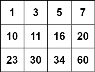
Input: matrix = [[1,3,5,7],[10,11,16,20],[23,30,34,60]], target = 13 Output: false
Constraints:
m =matrix.length=n =matrix[i].length=1 <m, n <= 100=-10=^{=4}= <= matrix[i][j], target <= 10=4
※ 2.5.3.1. Constraints and Edge Cases
- typical stuff, nothing fancy here, they’re asking for a boolean output (not the matrix cell coordinates itself)
- Here’s all the edge cases:
- Target smaller than all first elements (returns False).
- Target larger than all last elements (returns False).
- Empty matrix or empty rows (returns False).
※ 2.5.3.2. My Solution (Code)
1: from bisect import bisect_right 2: 3: class Solution: 4: │ def searchMatrix(self, matrix: List[List[int]], target: int) -> bool: 5: │ │ if not matrix or not matrix[0]: 6: │ │ │ return False 7: │ │ │ 8: │ │ # Find the row: last row whose first element <= target 9: │ │ col_vals = [row[0] for row in matrix] 10: │ │ row_idx = bisect_right(col_vals, target) - 1 11: │ │ if row_idx < 0: 12: │ │ │ return False 13: │ │ │ 14: │ │ # Search within the row 15: │ │ row = matrix[row_idx] 16: │ │ col_idx = bisect_left(row, target) 17: │ │ if col_idx < len(row) and row[col_idx] == target: 18: │ │ │ return True 19: │ │ return False
Here, we:
- use
bisect_rightto find the last row whose first element is<=target - then we use
bisect_leftto find the element within the row - Complexity analysis:
- Time Complexity:
- Building the first-column list: O(m)
- Binary search for row: O(log m)
- Binary search within row: O(log n)
- Total: O(log m + log n), which is slightly worse than the optimal O(log(m*n)) but still logarithmic and fast for the given constraints.
- Space Complexity:
- O(m) for the list of first elements (can be O(1) if you avoid building the list).
- Time Complexity:
- Some python improvements to this:
- use the unpacking operator instead of a listcomp
※ 2.5.3.2.1. Optimal Solution
Instead of trying to use the bisect functions, we can implement our “custom binary search function” here. We just need to treat the 2D array as a single flattened array since there’s actually a monotonically increasing order that we see.
That would give a runtime of \(O(log(m * n))\) and space usage of \(O(1)\)
1: class Solution: 2: │ def searchMatrix(self, matrix: List[List[int]], target: int) -> bool: 3: │ │ if not matrix or not matrix[0]: 4: │ │ │ return False 5: │ │ │ 6: │ │ m, n = len(matrix), len(matrix[0]) 7: │ │ left, right = 0, ( m * n ) - 1 8: │ │ 9: │ │ while left <= right: 10: │ │ │ mid = (left + right) // 2 11: │ │ │ # ⭐️ this is pretty! 12: │ │ │ row, col = divmod(mid, n) 13: │ │ │ val = matrix[row][col] 14: │ │ │ if val == target: 15: │ │ │ │ return True 16: │ │ │ elif val < target: 17: │ │ │ │ left = mid + 1 18: │ │ │ else: 19: │ │ │ │ right = mid - 1 20: │ │ return False
※ 2.5.3.2.2. Negative examples
Here’s a failing example. This is wrong because of the use of bisect_left instead of bisect_right
1: from bisect import bisect_left 2: class Solution: 3: │ def searchMatrix(self, matrix: List[List[int]], target: int) -> bool: 4: │ │ # approach for this is 2D binary searching, thisis because first column will be a jump index of sorts 5: │ │ # 1: find the row to look into 6: │ │ col_vals = [row[0] for row in matrix] 7: │ │ row_idx = bisect_left(col_vals, target) 8: │ │ 9: │ │ if (row_idx >= len(col_vals)): 10: │ │ │ return False 11: │ │ │ 12: │ │ # 2: search within the row 13: │ │ chosen_row_vals = [val for val in matrix[row_idx]] 14: │ │ col_idx = bisect_left(chosen_row_vals, target) 15: │ │ if col_idx >= len(chosen_row_vals): 16: │ │ │ return False 17: │ │ │ 18: │ │ return matrix[row_idx][col_idx] == target
You use bisectleft on the first column to find the row. However, bisect_left returns the index of the first element that is not less than the target. This means:
- If the target is exactly equal to a first-column value, you get the correct row.
- If the target is between two first-column values, you get the index of the next row above where the target could be (i.e., the row with a first-column value greater than the target).
- If the target is less than the first element, you get row 0 (which may not contain the target).
- If the target is greater than all first-column values, you get an out-of-bounds index.
Also, other problems:
chosen_row_vals = [val for val in matrix[row_idx]]is unnecessary. You can just usematrix[row_idx]directly. Don’t listcomp anyhow
※ 2.5.3.3. My Approach/Explanation
- Classic 2-step binary search happening here. The rows can be jumped to by searching amongst them first to pick a row and then we can search within the row.
※ 2.5.3.4. My Learnings/Questions
- It’s if performance was a consideration, then it would have been important to not jump into the implementation straight away and to first think about how to possibly reduce this to a 1D binary search.
- the divmod approach is really ingenious
- What are some ways to know when to use bisectleft vs bisectright?
On bisectleft vs bisectright
- When to use which:
bisect_left(a, x): Finds the first index where x could be inserted to maintain order (first element >= x).bisect_right(a, x): Finds the last index where x could be inserted to maintain order (first element > x).
- In this problem:
- You want the last row whose first element is ≤ target, so
bisect_rightis correct.
- You want the last row whose first element is ≤ target, so
- General rule:
- Use
bisect_leftwhen you want the leftmost position for a value. - Use
bisect_rightwhen you want the rightmost position for a value.
- Use
- When to use which:
※ 2.5.4. [24] Koko Eating Bananas (875)
Koko loves to eat bananas. There are n piles of bananas, the
i=^{=th} pile has piles[i] bananas. The guards have gone and will
come back in h hours.
Koko can decide her bananas-per-hour eating speed of k. Each hour, she
chooses some pile of bananas and eats k bananas from that pile. If the
pile has less than k bananas, she eats all of them instead and will
not eat any more bananas during this hour.
Koko likes to eat slowly but still wants to finish eating all the bananas before the guards return.
Return the minimum integer k such that she can eat all the bananas
within h hours.
Example 1:
Input: piles = [3,6,7,11], h = 8 Output: 4
Example 2:
Input: piles = [30,11,23,4,20], h = 5 Output: 30
Example 3:
Input: piles = [30,11,23,4,20], h = 6 Output: 23
Constraints:
1 <piles.length <= 10=4piles.length <h <= 10=91 <piles[i] <= 10=9
※ 2.5.4.1. Constraints and Edge Cases
- there initially was a question that I had about the meaning of
within: if it’s an inclusive or exclusive range. I realise that it’s an inclusive range. - input is not sorted
- there’s a fast return case: when the
number of piles=h, then we can early return because the slowest rate can only be equal to the biggest pile, so we found an early return for that.
※ 2.5.4.2. My Solution (Code)
Here’s the improved version which is iterative
1: class Solution: 2: │ def minEatingSpeed(self, piles: List[int], h: int) -> int: 3: │ │ max_pile = max(piles) 4: │ │ if h == len(piles): 5: │ │ │ return max_pile 6: │ │ │ 7: │ │ eating_time = lambda rate: sum((-(-pile//rate)) for pile in piles) 8: │ │ 9: │ │ left, right = 1, max_pile 10: │ │ 11: │ │ ans = right # will definitely reach this 12: │ │ while left <= right: 13: │ │ │ mid = left + ((right - left) // 2) 14: │ │ │ time = eating_time(mid) 15: │ │ │ if (time <= h): # fast enough but we wanna find slower rate 16: │ │ │ │ ans = mid # save this at least 17: │ │ │ │ right = mid - 1 18: │ │ │ else: 19: │ │ │ │ left = mid + 1 20: │ │ │ │ 21: │ │ return ans
Complexity:
- time
- each iteration of the search calls
eating_timethat runs in \(O(n)\) - search space is \([1, max(piles)]\) so the searching happens in \(O(log(max(piles)))\)
- TOTAL: \(O(n * log(max(piles))\)
- each iteration of the search calls
- space
- Iterative approach: \(O(1)\) since it’s just pointer manipulation
- in the inferior recursive approach below, the stack frames would have resulted in depth of \(O(log(max(piles)))\) which would have been the space usage.
Some improvements to this:
- no need to track answer because the left will be guaranteed to be the answer.
- we can inline the calculation instead of having a separate helper lambda
so a cleaner version is:
1: class Solution: 2: │ def minEatingSpeed(self, piles: List[int], h: int) -> int: 3: │ │ def hours_needed(rate): 4: │ │ │ return sum(-(-pile // rate) for pile in piles) # ceiling division 5: │ │ │ 6: │ │ left, right = 1, max(piles) 7: │ │ while left < right: 8: │ │ │ mid = (left + right) // 2 9: │ │ │ if hours_needed(mid) <= h: 10: │ │ │ │ right = mid 11: │ │ │ else: 12: │ │ │ │ left = mid + 1 13: │ │ return left
※ 2.5.4.2.1. Failed (slow, recursive) code
This solution passes base test cases but not all of them, it’s likely because of the recursion depth. Most likely this solution only accepts the iterative approach that saves space.
1: class Solution: 2: │ def minEatingSpeed(self, piles: List[int], h: int) -> int: 3: │ │ if h == len(piles): 4: │ │ │ return max(piles) 5: │ │ │ 6: │ │ def helper(left, right): 7: │ │ │ # calculate time taken with rate = mid 8: │ │ │ rate = left + ((right - left) // 2) 9: │ │ │ eating_time = sum((-(- pile// rate) for pile in piles)) 10: │ │ │ if eating_time == h: 11: │ │ │ │ return rate 12: │ │ │ elif eating_time > h: # too slow 13: │ │ │ │ return helper(rate + 1, right) 14: │ │ │ else: # too fast 15: │ │ │ │ return helper(left, rate - 1) 16: │ │ │ │ 17: │ │ return helper(1, max(piles))
I’m sure there are other flaws in this attempt as well
※ 2.5.4.3. My Approach/Explanation
The main thing is to first identify what we need to search. We need to search for the rate of eating, k. We know what its bounds will be: min 1 banana an hour and max would be the max(pile).
Also we can just directly used time as the determinant here.
※ 2.5.4.4. My Learnings/Questions
- remember that the first-reach should be the iterative implementation.
- careful not to get the basic calculations wrong. e.g. the time taken to eat = amount / rate
- For binary search problems:
- important to know what we are searching for always and whether we know the bounds of it.
- important to know the base case (when
left > right, that’s why the while condition is #SRCPYTHON{ while left <= right }) - the choice on which to recurse matters here.
- we want to find the SLOWEST rate, k. So even if the mid is fast enough, we still want to continue searching for something slower.
- python tips:
- so we know that floor division is
a//b - ceiling division is just the double negation of that so
-(-a//b)is ceiling negation.
- so we know that floor division is
Question: Could I have used the lambda as part of a
bisectfunction call? Or any other idiomatic way? Answer: Nope. The bisect function would work on a list, but the search space here (k) doesn’t have a list like that.The bisect module works on lists, not on a search space defined by a function. For “binary search on the answer” problems, you generally need to write your own binary search loop in Python.
the limitation of bisect functions are that the array must already exist. So suppose we were to search through the answer space, this won’t work because even if we supply a custom decider function as the key function.
bisectfunctions can’t:- Run user-defined monotonic checks (via a monotonic predicate) on candidate values.
- Search an implicit sorted space defined by a monotonic predicate rather than a concrete sorted list.
- Accept a custom comparator or key function (other than the element itself).
※ 2.5.5. [25] Find Minimum in Rotated Sorted Array (153) almost
Suppose an array of length n sorted in ascending order is rotated
between 1 and n times. For example, the array
nums = [0,1,2,4,5,6,7] might become:
[4,5,6,7,0,1,2]if it was rotated4times.[0,1,2,4,5,6,7]if it was rotated7times.
Notice that rotating an array [a[0], a[1], a[2], ..., a[n-1]] 1 time
results in the array [a[n-1], a[0], a[1], a[2], ..., a[n-2]].
Given the sorted rotated array nums of unique elements, return the
minimum element of this array.
You must write an algorithm that runs in O(log n) time.
Example 1:
Input: nums = [3,4,5,1,2] Output: 1 Explanation: The original array was [1,2,3,4,5] rotated 3 times.
Example 2:
Input: nums = [4,5,6,7,0,1,2] Output: 0 Explanation: The original array was [0,1,2,4,5,6,7] and it was rotated 4 times.
Example 3:
Input: nums = [11,13,15,17] Output: 11 Explanation: The original array was [11,13,15,17] and it was rotated 4 times.
Constraints:
n =nums.length=1 <n <= 5000=-5000 <nums[i] <= 5000=- All the integers of
numsare unique. numsis sorted and rotated between1andntimes.
※ 2.5.5.1. Constraints and Edge Cases
- nothing fancy to take note of, just needs to be binary search because it needs to run in \(O(log n)\) time.
※ 2.5.5.2. My Solution (Code)
※ 2.5.5.2.1. Initial Attempt (logical errors)
The approach is right with this one, just there’s some logical errors.
1: class Solution: 2: │ def findMin(self, nums: List[int]) -> int: 3: │ │ left, right = 0, len(nums) - 1 4: │ │ # early return if not rotated or rotate until recovered 5: │ │ │if (nums[left] < nums[right]): 6: │ │ │ return nums[left] 7: │ │ │ 8: │ │ while left <= right: 9: │ │ │ mid = left + ((right - left) // 2) 10: │ │ │ left_idx = mid - 1 if mid - 1 >= 0 else -1 11: │ │ │ right_idx = mid + 1 if mid + 1 < len(nums) else 0 12: │ │ │ is_valley = nums[left_idx] < nums[mid] and nums[mid] < nums[right_idx] 13: │ │ │ if is_valley: 14: │ │ │ │ return nums[mid] 15: │ │ │ elif nums[right_idx] < nums[-1]: # search into right segment 16: │ │ │ │ left = mid + 1 17: │ │ │ else: 18: │ │ │ │ right = mid - 1 19: │ │ │ │ 20: │ │ return nums[left]
Things done right:
- early return logic is right
Things done wrong:
- valley detection logic is wrong
is_valley = nums[left_idx] < nums[mid] and nums[mid] < nums[right_idx]does not correctly detect the minimum. The minimum is the only element smaller than its previous element (or first element in the array). - the updated bounds are wrong The way you update left and right is not standard for this problem and may miss the minimum in some cases.
※ 2.5.5.2.2. Corrected Attempt
- Intuition:
- what are we searching for? the min. So when we recurse, we need to know where the min would be:
- if
nums[mid] > nums[right]then the min is to the right of mid - if
nums[mid] <nums[right]= then the min is atmidor to the left ofmid
- if
- what are we searching for? the min. So when we recurse, we need to know where the min would be:
1: class Solution: 2: │ def findMin(self, nums: List[int]) -> int: 3: │ │ left, right = 0, len(nums) - 1 4: │ │ while left < right: 5: │ │ │ mid = left + (right - left) // 2 # overflow safe 6: │ │ │ # then the min must be in the right segment 7: │ │ │ if nums[mid] > nums[right]: 8: │ │ │ │ left = mid + 1 9: │ │ │ # min must be in the left segment 10: │ │ │ else: 11: │ │ │ │ right = mid 12: │ │ return nums[left]
Complexity:
- time is \(O(log n)\) because of the binary search
- space is \(O(1)\) because only using pointers
※ 2.5.5.3. My Approach/Explanation
I know that I need to implement a custom binary search. I’m searching for a valley point, that’s the point of rotation At each middle point I choose for the recursion step, I have 3 choices:
- I have found the valley
- I have not found the valley and I’m in the non-rotated part of the array ==> I need to search to the left of my mid
- I have not found the valley and I"m in the rotated part of the array ==> I need to search to the right of my mid
Correction:
- we need to know what we are looking for. it’s the min
- we need to know that at any point over the search, the min will DEFINITELY be withing our bounds (left, right)
- so each time, we just need to recurse either to right or left, eventualy we will find ourselves at the pivot point.
- there’s no need to find if mid is the pivot, explicit pivot check is unnecessary (check learnings below)
※ 2.5.5.4. My Learnings/Questions
- Intuition: The rotated array is two sorted subarrays. The minimum is the “pivot” point. We want to find the min and each time we know that min will be between our left and right boundaries. So when we choose to recurse, we need to make reference to the current window that we’re looking at.
- we should try to avoid custom valley logic, we should use the properties of the rotated array here. that’s how we get the intuition
- what are we searching for? the min. So when we recurse, we need to know where the min would be:
- if
nums[mid] > nums[right]then the min is to the right of mid - if
nums[mid] < nums[right]then the min is atmidor to the left ofmid
- if
- what are we searching for? the min. So when we recurse, we need to know where the min would be:
- calculating mid can be done in many ways, but not every way is overflow-safe (for other languages)
- overflow safe, correct:
mid = left + ((right - left) // 2). this only matters for fixed-integer languages (Java, C++) - overflow unsafe, correct:
mid = (left + right) // 2
- overflow safe, correct:
An explicit pivot check is unnecessary:
Show/Hide Md CodeYou **do not need to explicitly check if `mid` is the pivot** (i.e., directly test if `nums[mid]` is less than both neighbors) in the sample optimal solution for finding the minimum in a rotated sorted array because the **binary search logic naturally converges to the pivot** by exploiting the sorted properties of the array. ### Why this works - In a rotated sorted array, one half is always sorted. - By comparing `nums[mid]` to `nums[right]`: │ - If `nums[mid] > nums[right]`, the minimum **must** be to the right of `mid` (because the rotation point is in the right half). │ - If `nums[mid] ...the minimum is the "pivot" point. > Focus on comparing `nums[mid]` with `nums[right]` to decide which half to search. > The "valley" logic is not necessary and can be error-prone. ### Summary Table | Approach | Need to Check Neighbors? | Robust? | Simpler? | |-------------------------------|:------------------------:|:-------:|:--------:| | Compare `nums[mid]` to `right`| No | Yes | Yes | | Explicit pivot neighbor check | Yes | No | No | **In short:** The binary search method that compares `nums[mid]` to `nums[right]` always narrows the search to the pivot, so you don't need to check neighbors or explicitly find the pivot[7]. [1] https://www.geeksforgeeks.org/search-an-element-in-a-sorted-and-pivoted-array/ [2] https://stackoverflow.com/questions/73148061/find-key-index-in-a-rotated-sorted-array-using-binary-sort [3] https://takeuforward.org/data-structure/search-element-in-a-rotated-sorted-array/ [4] https://leetcode.com/problems/search-in-rotated-sorted-array/ [5] https://www.geeksforgeeks.org/dsa/check-if-an-array-is-sorted-and-rotated-using-binary-search/ [6] https://www.w3resource.com/data-structures-and-algorithms/array/dsa-search-in-a-rotated-sorted-array.php [7] https://github.com/Shaldonbarnes10/Rotated-Sorted-Array-Search-in-Cpp-binary-search-technique [8] https://dev.to/mostafa_/building-a-rotated-sorted-array-search-in-java-understanding-pivot-and-binary-search-3k5f [9] https://leetcode.com/problems/search-in-rotated-sorted-array-ii/ [10] https://neetcode.io/problems/find-target-in-rotated-sorted-array
※ 2.5.6. [26] Time Based Key Value Store (981)
Design a time-based key-value data structure that can store multiple values for the same key at different time stamps and retrieve the key’s value at a certain timestamp.
Implement the TimeMap class:
TimeMap()Initializes the object of the data structure.void set(String key, String value, int timestamp)Stores the keykeywith the valuevalueat the given timetimestamp.String get(String key, int timestamp)Returns a value such thatsetwas called previously, withtimestamp_prev <timestamp=. If there are multiple such values, it returns the value associated with the largesttimestamp_prev. If there are no values, it returns"".
Example 1:
Input
["TimeMap", "set", "get", "get", "set", "get", "get"]
[[], ["foo", "bar", 1], ["foo", 1], ["foo", 3], ["foo", "bar2", 4], ["foo", 4], ["foo", 5]]
Output
[null, null, "bar", "bar", null, "bar2", "bar2"]
Explanation
TimeMap timeMap = new TimeMap();
timeMap.set("foo", "bar", 1); // store the key "foo" and value "bar" along with timestamp = 1.
timeMap.get("foo", 1); // return "bar"
timeMap.get("foo", 3); // return "bar", since there is no value corresponding to foo at timestamp 3 and timestamp 2, then the only value is at timestamp 1 is "bar".
timeMap.set("foo", "bar2", 4); // store the key "foo" and value "bar2" along with timestamp = 4.
timeMap.get("foo", 4); // return "bar2"
timeMap.get("foo", 5); // return "bar2"
Constraints:
1 <key.length, value.length <= 100=keyandvalueconsist of lowercase English letters and digits.1 <timestamp <= 10=7- All the timestamps
timestampofsetare strictly increasing. - At most
2 * 10=^{=5} calls will be made tosetandget.
※ 2.5.6.1. Constraints and Edge Cases
- remember that the null case return is
"" - we don’t need to account for input handling based on the constraints given
- the timestamps are strictly increasing – no duplicates + we can keep appending without caring about where to insert the values
※ 2.5.6.2. My Solution (Code)
1: from collections import defaultdict 2: from bisect import bisect_right 3: 4: class TimeMap: 5: │ 6: │ def __init__(self): 7: │ │ self.key_to_vals = defaultdict(list) 8: │ │ 9: │ def set(self, key: str, value: str, timestamp: int) -> None: 10: │ │ self.key_to_vals[key].append((timestamp, value)) 11: │ │ 12: │ def get(self, key: str, timestamp: int) -> str: 13: │ │ vals = self.key_to_vals[key] 14: │ │ if not vals: 15: │ │ │ return "" 16: │ │ │ 17: │ │ idx = bisect_right(vals, timestamp, key=lambda x: x[0]) 18: │ │ if idx == 0: 19: │ │ │ return "" 20: │ │ │ 21: │ │ return vals[idx-1][1]
Complexity Analysis:
- time
setis in \(O(1)\) amortized because it’s just a list appendgetis in \(O(log n)\) per query because of the binary search (nis the current number of values for the key)
- space:
- \(O(N)\) where
Nis the total number ofsetoperations (because we store every value for every key)
- \(O(N)\) where
Here’s one that is compatible with python <3.10:
1: from collections import defaultdict 2: from bisect import bisect_right 3: 4: class TimeMap: 5: │ def __init__(self): 6: │ │ self.key_to_vals = defaultdict(list) 7: │ │ 8: │ def set(self, key: str, value: str, timestamp: int) -> None: 9: │ │ self.key_to_vals[key].append((timestamp, value)) 10: │ │ 11: │ def get(self, key: str, timestamp: int) -> str: 12: │ │ vals = self.key_to_vals[key] 13: │ │ if not vals: 14: │ │ │ return "" 15: │ │ # Extract timestamps for binary search 16: │ │ timestamps = [t for t, _ in vals] 17: │ │ idx = bisect_right(timestamps, timestamp) 18: │ │ if idx == 0: 19: │ │ │ return "" 20: │ │ return vals[idx-1][1]
※ 2.5.6.2.1. Slow but acceptable version
This is definitely a binary search problem and that’s how we should answer it. For some reason, an alternative where we use a priority queue also exists. I guess that’s more of if the insertion order is not chrono-guaranteed.
this has unnecessary operations.
1: import heapq 2: 3: class TimeMap: 4: │ def __init__(self): 5: │ │ self.store = {} 6: │ │ 7: │ def set(self, key: str, value: str, timestamp: int) -> None: 8: │ │ if key not in self.store: 9: │ │ │ self.store[key] = [] 10: │ │ │ 11: │ │ # Push negated timestamp and value into the list 12: │ │ heapq.heappush(self.store[key], (-timestamp, value)) 13: │ │ 14: │ def get(self, key: str, timestamp: int) -> str: 15: │ │ if key not in self.store: 16: │ │ │ return "" 17: │ │ │ 18: │ │ # Access the max-heap for this key 19: │ │ inner_pq = self.store[key] 20: │ │ 21: │ │ # Iterate through the heap until we find a valid timestamp 22: │ │ other_pq = [] 23: │ │ while inner_pq: 24: │ │ │ neg_timestamp, value = heapq.heappop(inner_pq) 25: │ │ │ actual_timestamp = -neg_timestamp 26: │ │ │ 27: │ │ │ if actual_timestamp <= timestamp: 28: │ │ │ │ # Push it back since we might need it later 29: │ │ │ │ heapq.heappush(other_pq, (neg_timestamp, value)) 30: │ │ │ │ self.store[key] = other_pq 31: │ │ │ │ return value 32: │ │ │ │ 33: │ │ │ heapq.heappush(other_pq, (neg_timestamp, value)) 34: │ │ │ 35: │ │ self.store[key] = other_pq 36: │ │ return "" 37: │ │ 38: │ │ 39: │ │ 40: # Your TimeMap object will be instantiated and called as such: 41: # obj = TimeMap() 42: # obj.set(key,value,timestamp) 43: # param_2 = obj.get(key,timestamp)
※ 2.5.6.3. My Approach/Explanation
- This is a overloading of dictionary to act as a multi-set. Chrono-order is what keeps things well-ordered.
- So we just need to keep a list of tuples for each key
- the insertion can just happen via
appendsbecause of the chrono order. - We just need to binary search through the chronolist that we keep.
※ 2.5.6.4. My Learnings/Questions
- I know that python 3.10+ allows bisect to take in a
keyargument, this an iterator to figure out what to use for the ordering (not how to order it). That’s what I’ve used here for my solution. If for some reason, we are unable to use that, we can manually extract out the timestamps from thevalstuple and use the relative indexing for it. - careful on the empty return cases, don’t do the wrong type (
Noneinstead of the correct"") - Alternative Data Structures:
- You could use a balanced BST or skip list for each key to allow O(log n) insertion and search, but this is unnecessary since the strictly increasing timestamp property makes appending and binary search optimal
- Intuition:
- The problem reduces to “for a given sorted list, find the rightmost value ≤ target,” which is classic for binary search.
※ 2.5.7. TODO [27] Median of two sorted arrays [4] redo hard binary_search median virtual_domain
Given two sorted arrays nums1 and nums2 of size m and n
respectively, return the median of the two sorted arrays.
The overall run time complexity should be O(log (m+n)).
Example 1:
Input: nums1 = [1,3], nums2 = [2] Output: 2.00000 Explanation: merged array = [1,2,3] and median is 2.
Example 2:
Input: nums1 = [1,2], nums2 = [3,4] Output: 2.50000 Explanation: merged array = [1,2,3,4] and median is (2 + 3) / 2 = 2.5.
Constraints:
nums1.length =m=nums2.length =n=0 <m <= 1000=0 <n <= 1000=1 <m + n <= 2000=-10=^{=6}= <= nums1[i], nums2[i] <= 10=6
※ 2.5.7.1. Constraints and Edge Cases
- it must run in \(O(log(m + n)) = O(log(m) * log(n))\) time.
- so it has to be a binary search approach
- so it has to avoid explicit merges
※ 2.5.7.2. My Solution (Code)
※ 2.5.7.2.1. Optimal code (iterative binary search)
this code is copied, I have to come back to this to make this more intuitive, I don’t agree with the way it’s written, it could make the intuition clearer.
1: class Solution: 2: │ def findMedianSortedArrays(self, nums1, nums2): 3: │ │ # Ensure nums1 is the smaller array 4: │ │ if len(nums1) > len(nums2): 5: │ │ │ nums1, nums2 = nums2, nums1 6: │ │ │ 7: │ │ m, n = len(nums1), len(nums2) 8: │ │ total = m + n 9: │ │ half = total // 2 10: │ │ 11: │ │ left, right = 0, m 12: │ │ while True: 13: │ │ │ i = (left + right) // 2 # Partition in nums1 14: │ │ │ j = half - i # Partition in nums2 15: │ │ │ 16: │ │ │ nums1_left = nums1[i-1] if i > 0 else float('-inf') 17: │ │ │ nums1_right = nums1[i] if i < m else float('inf') 18: │ │ │ nums2_left = nums2[j-1] if j > 0 else float('-inf') 19: │ │ │ nums2_right = nums2[j] if j < n else float('inf') 20: │ │ │ 21: │ │ │ # Found correct partition 22: │ │ │ if nums1_left <= nums2_right and nums2_left <= nums1_right: 23: │ │ │ │ if total % 2: 24: │ │ │ │ │ return min(nums1_right, nums2_right) 25: │ │ │ │ return (max(nums1_left, nums2_left) + min(nums1_right, nums2_right)) / 2 26: │ │ │ elif nums1_left > nums2_right: 27: │ │ │ │ right = i - 1 28: │ │ │ else: 29: │ │ │ │ left = i + 1
※ 2.5.7.2.2. failed attempt
Frankly, I’m clue-less here.
1: class Solution: 2: │ def findMedianSortedArrays(self, nums1: List[int], nums2: List[int]) -> float: 3: │ │ get_med = lambda ls: ls[(len(ls) - 1) / 2] if len(ls) % 2 == 1 else (ls[len(ls) // 2] + ls[(len(ls) // 2) + 1]) / 2 4: │ │ med_1, med_2 = get_med(nums1), get_med(nums2) 5: │ │ # fix med_1, see if it falls to the L or R of med_2 6: │ │ is_med_1_smaller = med_1 < med_2
※ 2.5.7.3. My Approach/Explanation
I have no idea how to do this. My first-reach was that we need to consider how the two medians shift when merging happens.
I had the following questions:
- can I avoid merging?
- not sure, I don’t have a fast way of merging two sorted arrays
- I have to avoid merging because any merging will have to happen in \(O(m + n)\) time and that will make it slow already.
- will there be overlaps in values from the two arrays? and duplicates
- I think this is a yes to both
- The return value of float implies that we’d need to handle both the cases of a merged array being even numbered and odd numbered
I think these hold true:
- We HAVE to avoid merging
- we need to search binary search to do so efficiently
※ 2.5.7.4. My Learnings/Questions
- Key intuition for the optimal solution:
medianis less about the value, more about the ordering of the elements, the juxtaposion of position-based info with content based info should not throw us off-guard- for median, remember to think of it as partitioning
- we need to keep thinking about the partitioning of the two
- We need to partition both array such that the left half = right half or left half is one more than the right half
- Some implementation reminders:
- always binary search on the shorter array for efficiency
- We need to look for the partition point
- The neetcode video is a good walkthrough of the problem with good visualisation on it
※ 2.5.7.5. Prompt for GPT Evaluation
Please do the following:
- Evaluate the correctness of my solution. Are there any logical or edge case errors?
- Analyze the time and space complexity of my code.
- Suggest improvements in code style, efficiency, or clarity.
- Compare my approach to the optimal solution (if different).
- Provide a sample optimal solution (if mine is not optimal).
- Point out any Pythonic (or language-specific) improvements.
Are there any completely different approaches to this problem?
- e.g something that uses a completely different data structure
If so, then help me gain the intuition for it and show the code clearly
- Answer my specific questions (if any are listed above).
※ 2.5.7.6. Additional Context
So while I missed the key intuition here, the other things such as knowing that the merging should be avoided and other inferences were done correctly and that’s something to be happy about.
※ 2.5.8. [Depth 1] Capacity to Ship Packages within D Days (1011) left_boundary_finding binary_search
A conveyor belt has packages that must be shipped from one port to
another within days days.
The i=^{=th} package on the conveyor belt has a weight of
weights[i]. Each day, we load the ship with packages on the conveyor
belt (in the order given by weights). We may not load more weight than
the maximum weight capacity of the ship.
Return the least weight capacity of the ship that will result in all the
packages on the conveyor belt being shipped within days days.
Example 1:
Input: weights = [1,2,3,4,5,6,7,8,9,10], days = 5 Output: 15 Explanation: A ship capacity of 15 is the minimum to ship all the packages in 5 days like this: 1st day: 1, 2, 3, 4, 5 2nd day: 6, 7 3rd day: 8 4th day: 9 5th day: 10 Note that the cargo must be shipped in the order given, so using a ship of capacity 14 and splitting the packages into parts like (2, 3, 4, 5), (1, 6, 7), (8), (9), (10) is not allowed.
Example 2:
Input: weights = [3,2,2,4,1,4], days = 3 Output: 6 Explanation: A ship capacity of 6 is the minimum to ship all the packages in 3 days like this: 1st day: 3, 2 2nd day: 2, 4 3rd day: 1, 4
Example 3:
Input: weights = [1,2,3,1,1], days = 4 Output: 3 Explanation: 1st day: 1 2nd day: 2 3rd day: 3 4th day: 1, 1
Constraints:
1 <days <= weights.length <= 5 * 10=41 <weights[i] <= 500=
※ 2.5.8.1. Constraints and Edge Cases
- just know that there will at least be 1 trip, so the base value for trip when calculating is 1.
※ 2.5.8.2. My Solution (Code)
※ 2.5.8.2.1. v0: correct optimal
1: class Solution: 2: │ def shipWithinDays(self, weights: List[int], days: int) -> int: 3: │ │ def get_days(capacity): 4: │ │ │ num_trips = 1 # GOTCHA (logical): at least one trip needed 5: │ │ │ curr_load = 0 6: │ │ │ for w in weights: 7: │ │ │ │ if curr_load + w > capacity: 8: │ │ │ │ │ num_trips += 1 9: │ │ │ │ │ curr_load = w 10: │ │ │ │ else: 11: │ │ │ │ │ curr_load += w 12: │ │ │ │ │ 13: │ │ │ return num_trips 14: │ │ │ 15: │ │ low = min_capacity = max(weights) # else we can't even bring this package over 16: │ │ high = sum(weights) # then we can just take it all in one go 17: │ │ 18: │ │ ans = high 19: │ │ # inclusive ranges: 20: │ │ while low <= high: 21: │ │ │ mid = low + (high - low) // 2 22: │ │ │ if get_days(mid) <= days: 23: │ │ │ │ # restrict the search on a smaller space: 24: │ │ │ │ high = mid - 1 25: │ │ │ │ ans = mid 26: │ │ │ else: 27: │ │ │ │ low = mid + 1 28: │ │ │ │ 29: │ │ return ans
- Approach: leverages the binary search over the answer space (capacity) combined with a greedy check for feasibility
- This problem exhibits some greedy decision making. The greedy strategy helps determine feasibility given a fixed capacity by packing packages in order until the capacity is reached, then shipping on the next day. The binary search optimizes the capacity.
- Greedy framework:
- Choice: Ship as many packages as possible without exceeding capacity each day.
- Feasibility Check: Can all packages be shipped within days at capacity mid?
- Optimization: Use binary search on capacity to find the minimal capacity with feasible shipping.
- Greedy framework:
- Time Complexity: \(O(N log S)\), where \(N\) is the number of packages and \(S\) is the sum of weights.
- The binary search runs in \(O(log S)\) steps.
- Each getdays call runs in \(O(N)\).
- Space Complexity: \(O(1)\), only variables and counters are used; no extra space proportional to input size.
※ 2.5.8.3. My Approach/Explanation
This is a classic find left boundary to fulfill some custom predicate kind of question.
※ 2.5.8.4. My Learnings/Questions
- the helper function had the logical GOTCHA that I fell for: the number of trips is at least 1 regardless of the capacity)
※ 2.5.8.5. Prompt for GPT Evaluation
Please do the following:
- Evaluate the correctness of my solution. Are there any logical or edge case errors?
- Analyze the time and space complexity of my code.
- Suggest improvements in code style, efficiency, or clarity.
- Compare my approach to the optimal solution (if different).
- Provide a sample optimal solution (if mine is not optimal).
- Point out any Pythonic (or language-specific) improvements.
Are there any completely different approaches to this problem?
- e.g something that uses a completely different data structure
If so, then help me gain the intuition for it and show the code clearly
- Answer my specific questions (if any are listed above).
※ 2.5.8.6. Prompt for GPT Evaluation (with Greedy)
Please do the following:
- Evaluate the correctness of my solution. Are there any logical or edge case errors?
- Analyze the time and space complexity of my code.
- Suggest improvements in code style, efficiency, or clarity.
- Compare my approach to the optimal solution (if different).
- Provide a sample optimal solution (if mine is not optimal).
- Point out any Pythonic (or language-specific) improvements.
Are there any completely different approaches to this problem?
- e.g something that uses a completely different data structure
If so, then help me gain the intuition for it and show the code clearly
- Answer my specific questions (if any are listed above).
ALso help me evaluate this in the context of greedy algorithms, ensuring that a good framework of presenting this problem into a greedy algo is given / understood.
※ 2.5.8.7. Prompt for GPT Evaluation (with DP)
Please do the following:
- Evaluate the correctness of my solution. Are there any logical or edge case errors?
- Analyze the time and space complexity of my code.
- Suggest improvements in code style, efficiency, or clarity.
- Compare my approach to the optimal solution (if different).
- Provide a sample optimal solution (if mine is not optimal).
- Point out any Pythonic (or language-specific) improvements.
Are there any completely different approaches to this problem?
- e.g something that uses a completely different data structure
If so, then help me gain the intuition for it and show the code clearly
- Answer my specific questions (if any are listed above).
ALso help me evaluate this in the context of greedy algorithms, ensuring that a good framework of presenting this problem into a greedy algo is given / understood.
Additionally, use my notes for Dynamic Programming and use the recipes that are here.
Recipe to define a solution via DP
[Generate Naive Recursive Algo]
Characterise the structure of an optimal solution \(\implies\) what are the subproblems? \(\implies\) are they independent subproblems? \(\implies\) how many subproblems will there be?
- Recursively define the value of an optimal solution \(\implies\) does this have the overlapping sub-problems property? \(\implies\) what’s the cost of making a choice? \(\implies\) how many ways can I make that choice?
- Compute value of an optimal solution
- Construct optimal solution from computed information Defining things
- Optimal Substructure:
A problem exhibits “optimal substructure” if an optimal solution to the problem contains within it optimal solutions to subproblems.
Elements of Dynamic Programming: Key Indicators of Applicability [1] Optimal Sub-Structure Defining “Optimal Substructure” A problem exhibits optimal substructure if an optimal solution to the problem contains within it optimal solutions to sub-problems.
- typically a signal that DP (or Greedy Approaches) will apply here.
- this is something to discover about the problem domain Common Pattern when Discovering Optimal Substructure
solution involves making a choice e.g. choosing an initial cut in the rod or choosing what k should be for splitting the matrix chain up
\(\implies\) making the choice also determines the number of sub-problems that the problem is reduced to
- Assume that the optimal choice can be determined, ignore how first.
- Given the optimal choice, determine what the sub-problems looks like \(\implies\) i.e. characterise the space of the subproblems
- keep the space as simple as possible then expand
typically the substructures vary across problem domains in 2 ways:
[number of subproblems]
how many sub-problems does an optimal solution to the original problem use?
- rod cutting:
# of subproblems = 1(of size n-i) where i is the chosen first cut lengthmatrix split:
# of subproblems = 2(left split and right split)[number of subproblem choices]
how many choices are there when determining which subproblems(s) to use in an optimal solution. i.e. now that we know what to choose, how many ways are there to make that choice?
- rod cutting: # of choices for i = length of first cut,
nchoices- matrix split: # of choices for where to split (idx k) =
j - iNaturally, this is how we analyse the runtime:
# of subproblems * # of choices @ each sub-problem- Reason to yourself if and how solving the subproblems that are used in an optimal solution means that the subproblem-solutions are also optimal. This is typically done via the
cut-and-paste argument.Caveat: Subproblems must be
independent
- “independent subproblems”
- solution to one subproblem doesn’t affect the solution to another subproblem for the same problem
example: Unweighted Shortest Path (independent subproblems) vs Unweighted Longest Simple Path (dependent subproblems)
Consider graph \(G = (V,E)\) with vertices \(u,v \notin V\)
- Unweighted shortest path: we want to find path \(u\overset{p}{\leadsto}v\) then we can break it down into subpaths \(u\overset{p1}{\leadsto}w\overset{p2}{\leadsto}v\) (optimal substructure). If path, p, is optimal from \(u\leadsto{v}\) then p1 must be shortest path from \(u\leadsto{w}\) and likewise p2 must be shortest path from \(w\leadsto{v}\) (cut-and-paste argument) Here, we know that the subproblems are independent.
- Unweighted Longest Simple Path: the subproblems can have paths that overlap (not subproblem overlap), hence it’s not independent because the vertices that appear can appear in the solution to the second subproblem
Terminology: Optimal substruture vs optimal solution optimal substructure is a property that enables efficient computation of the optimal value, while the solution is the specific configuration that yields that optimal value
You’re right that in dynamic programming algorithms for optimization problems, the goal is usually to find an optimal solution rather than the unique optimal solution. Here’s how the optimal substructure and the actual solution differ:
### Optimal Substructure
The optimal substructure refers to the property that the optimal solution to a problem can be constructed from the optimal solutions to its subproblems. This means that if we know the optimal solutions to the subproblems, we can efficiently determine the optimal solution to the overall problem.
For example, in the rod cutting problem, if we know the maximum revenue for rods of length 1 to n-1, we can efficiently determine the maximum revenue for a rod of length n by considering cutting the rod at each possible length and taking the maximum revenue.
### The Solution
The actual solution, on the other hand, refers to the specific configuration or set of choices that yields the optimal value. In the rod cutting problem, the solution would be the specific way to cut the rod that results in the maximum revenue.
The key difference is that the optimal substructure allows us to efficiently compute the optimal value, but it doesn’t necessarily specify the exact solution. There may be multiple solutions that yield the same optimal value.
For example, in the rod cutting problem, there may be multiple ways to cut the rod that result in the same maximum revenue. The optimal substructure allows us to efficiently compute the maximum revenue, but it doesn’t specify which particular cutting configuration to choose.
So in summary, the optimal substructure is a property that enables efficient computation of the optimal value, while the solution is the specific configuration that yields that optimal value. Dynamic programming algorithms leverage the optimal substructure to efficiently compute the optimal value, but the actual solution may not be uniquely determined.
Citations: [1] https://library.fiveable.me/key-terms/programming-for-mathematical-applications/optimal-substructure [2] https://afteracademy.com/blog/optimal-substructure-and-overlapping-subproblems/ [3] https://www.geeksforgeeks.org/optimal-substructure-property-in-dynamic-programming-dp-2/ [4] https://labuladong.gitbook.io/algo-en/i.-dynamic-programming/optimalsubstructure [5] https://stackoverflow.com/questions/33563230/optimal-substructure-in-dynamic-programing [6] https://en.wikipedia.org/wiki/Optimal_substructure [7] https://www.cs.cmu.edu/~15451-f22/lectures/lec09-dp1.pdf [8] https://www.javatpoint.com/optimal-substructure-property
[2] Overlapping Sub-Problems
- DP should be disambiguated from Divide & Conquer:
- for Divide&Conquer, choosing a division point generates brand new problems that likely don’t overlap
- for DP, the space of sub-problems is small and hence if done purely recursively, the same operations get computed multiple times
[Practical point] Reconstructing an optimal solution Since one way to look at DP is table-filling, we typically have:
- table of costs
- table of optimal choices
the table of optimal choices can be built from the table of costs, but we want to avoid recalculating the optimal choices
Memoisation as an alternative
- the textbook used sees this as an alternative and memoised tables as the aux DS for recursive, top-down approaches
- memoisation also exploits the observation that the space of the subproblems is small and hence overlapping
Common Misconceptions Here are some common misconception, based on what perplexity says
Based on the search results, here are some of the common misconceptions that learners have about dynamic programming:
## 1. Misconceptions about the Definition and Purpose of Dynamic Programming
- Thinking that recursion and dynamic programming are explicitly different concepts[3].
- Believing that dynamic programming is exclusively used to solve optimization problems[3].
## 2. Misconceptions about the Optimal Substructure Property
- Assuming that the optimal solution to a problem can be constructed from any combination of optimal solutions to its subproblems, rather than specific optimal solutions to the right subproblems[1][2].
- Thinking that the optimal solution to a problem can be constructed from optimal solutions to unrelated subproblems[4].
## 3. Misconceptions about Memoization and Tabulation
- Failing to recognize that memoization (top-down) and tabulation (bottom-up) are two different implementation strategies for dynamic programming[1][2].
- Believing that memoization always involves recursion and tabulation always involves iteration[1][2].
## 4. Misconceptions about the Filling Order of the DP Table
- Assuming that the DP table must always be filled in a specific order (e.g., always from small to big cases), without understanding that the order depends on the problem’s dependencies and constraints[1][2][4].
## 5. Misconceptions about the Relationship between Subproblems
- Thinking that the solutions to all subproblems are needed to solve the original problem, rather than understanding that only specific optimal solutions to the right subproblems are needed[1][2].
## 6. Misconceptions about the Efficiency of Dynamic Programming
- Believing that dynamic programming always leads to polynomial-time algorithms, without understanding that it can sometimes only slightly improve the exponential-time complexity[4].
Understanding and addressing these common misconceptions can help learners develop a more accurate and comprehensive understanding of dynamic programming and its applications.
Citations: [1] https://dl.acm.org/doi/10.1145/3159450.3159528 [2] https://dl.acm.org/doi/abs/10.1145/3159450.3159528 [3] https://ics.uci.edu/~mikes/papers/Student_Misconceptions_Dynamic_Programming.pdf [4] https://www.cs.cmu.edu/~15451-f22/lectures/lec09-dp1.pdf [5] https://www.reddit.com/r/compsci/comments/er05hn/help_me_wrap_my_head_around_dynamic_programming/ [6] https://yourbasic.org/algorithms/dynamic-programming-explained/ [7] https://stackoverflow.com/questions/33563230/optimal-substructure-in-dynamic-programing [8] https://lec.inf.ethz.ch/DA/2020/slides/daLecture13.en.pdf
Greedy Algos vs DP When comparing greedy strategies and dynamic programming (DP), it’s essential to understand how they differ in methodology, application, and the nature of the problems they solve. Both approaches involve identifying optimal substructures, but they apply this concept in distinct ways. Here’s a detailed disambiguation based on the search results:
### 1. Definition and Approach
- Greedy Strategy:
- A greedy algorithm makes the most optimal choice at each step with the hope that these local optimum choices will lead to a global optimum solution. It does not consider the overall impact of the current choice on future decisions.
- Greedy algorithms are typically simpler and faster to implement, as they do not require storing results of subproblems. However, they do not guarantee an optimal solution for all problems.
- Dynamic Programming:
- Dynamic programming is a technique used to solve complex problems by breaking them down into simpler subproblems. It is based on the principles of optimal substructure and overlapping subproblems.
- DP guarantees an optimal solution by considering all possible cases and storing the results of subproblems to avoid redundant computations. This can lead to higher time and space complexity compared to greedy algorithms.
### 2. Optimal Substructure
- Greedy Algorithms:
- Greedy algorithms rely on the greedy choice property, which means that a locally optimal choice leads to a globally optimal solution. However, this property does not hold for all problems, which is why greedy algorithms may fail to find the optimal solution in some cases.
- Dynamic Programming:
- Dynamic programming explicitly uses the optimal substructure property, where an optimal solution to a problem can be constructed from optimal solutions of its subproblems. DP ensures that all relevant subproblems are considered, leading to a guaranteed optimal solution.
### 3. Subproblem Reuse
- Greedy Strategy:
- Greedy algorithms typically do not reuse solutions to subproblems. Each decision is made independently based on the current state without revisiting previous choices.
- Dynamic Programming:
- DP explicitly solves and caches solutions to overlapping subproblems. This reuse of subproblem solutions is a key feature of dynamic programming, allowing for efficient computation.
### 4. Complexity and Efficiency
- Greedy Algorithms:
- Greedy algorithms are generally more efficient in terms of time complexity due to their straightforward approach. They often run in linear or logarithmic time, depending on the problem.
- They are suitable for problems where local optimization leads to global optimization, such as in minimum spanning trees or certain shortest path problems.
- Dynamic Programming:
- DP can be less efficient than greedy algorithms in terms of time complexity, especially if every possible solution is computed. However, proper use of memoization can mitigate this.
- DP is applicable to problems with overlapping subproblems and optimal substructure, such as the Fibonacci sequence, longest common subsequence, or knapsack problems.
### 5. Examples
- Greedy Algorithms:
- Common examples include:
- Fractional Knapsack Problem: Where you can take fractions of items.
- Minimum Spanning Tree: Algorithms like Prim’s and Kruskal’s.
- Huffman Coding: For optimal prefix codes.
- Dynamic Programming:
- Common examples include:
- 0/1 Knapsack Problem: Where you cannot take fractions of items.
- Longest Common Subsequence: Finding the longest subsequence present in both sequences.
- Matrix Chain Multiplication: Finding the most efficient way to multiply a given sequence of matrices.
### Conclusion
In summary, while both greedy strategies and dynamic programming involve the concept of optimal substructure, they differ significantly in their approach to problem-solving. Greedy algorithms make decisions based on local optimality without revisiting previous choices, whereas dynamic programming systematically considers all possible subproblems and their solutions to ensure a globally optimal result. Understanding these differences allows for better problem-solving strategies and the appropriate application of each method based on the problem’s characteristics.
Citations: [1] https://www.boardinfinity.com/blog/greedy-vs-dp/ [2] https://www.shiksha.com/online-courses/articles/difference-between-greedy-and-dynamic-programming-blogId-158053 [3] https://www.interviewbit.com/blog/difference-between-greedy-and-dynamic-programming/ [4] https://stackoverflow.com/questions/16690249/what-is-the-difference-between-dynamic-programming-and-greedy-approach [5] https://www.geeksforgeeks.org/greedy-approach-vs-dynamic-programming/ [6] https://byjus.com/gate/difference-between-greedy-approach-and-dynamic-programming/ [7] https://www.cs.cmu.edu/~15451-f22/lectures/lec09-dp1.pdf [8] https://ics.uci.edu/~mikes/papers/Student_Misconceptions_Dynamic_Programming.pdf
General Takeaways Bottom-up vs Top-Down
- we can use a subproblem graph to show the relationship with the subproblems ==> diff b/w bottom up and top-down is how these deps are handled (recursive-called or soundly iterated with a proper direction)
- aysymptotic runtime is pretty similar since both solve similar \(\Omega(n^{2})\)
- Bottom up:
- basically considers order at which the subproblems are solved
- because of the ordered way of solving the smaller sub-problems first, there’s no need for recursive calls and code can be iterative entirely
- so no overhead from function calls
- no chance of stack overflow
- benefits from data-locality
- a way to see the vertices of the subproblem graph such that the subproblems y-adjacent to a given subproblem x is solved before subproblem x is solved
※ 2.5.8.8. [Optional] Additional Context
<e.g., “I struggled with X”, “I want to know about alternative algorithms”, etc.>
※ 2.5.9. [Depth 2] Find Minimum in Rotated Sorted Array II (154) hard binary_search rotated_array
Suppose an array of length n sorted in ascending order is rotated
between 1 and n times. For example, the array
nums = [0,1,4,4,5,6,7] might become:
[4,5,6,7,0,1,4]if it was rotated4times.[0,1,4,4,5,6,7]if it was rotated7times.
Notice that rotating an array [a[0], a[1], a[2], ..., a[n-1]] 1 time
results in the array [a[n-1], a[0], a[1], a[2], ..., a[n-2]].
Given the sorted rotated array nums that may contain duplicates,
return the minimum element of this array.
You must decrease the overall operation steps as much as possible.
Example 1:
Input: nums = [1,3,5] Output: 1
Example 2:
Input: nums = [2,2,2,0,1] Output: 0
Constraints:
n =nums.length=1 <n <= 5000=-5000 <nums[i] <= 5000=numsis sorted and rotated between1andntimes.
Follow up: This problem is similar
to Find
Minimum in Rotated Sorted Array, but nums may contain duplicates.
Would this affect the runtime complexity? How and why?
※ 2.5.9.1. Constraints and Edge Cases
<list constraints, input limits, or tricky edge cases here>
※ 2.5.9.2. My Solution (Code)
※ 2.5.9.2.1. v1: correct, optimal
The key idea is that same as usual binary search: which segment do we confidently recurse into? Turns out that we can compare boundaries with the mid: if right is smaller than mid then the min value must be @ right segment, if right is larger than mid, then the min value must come from the left segment and if it’s equal, then we have to pop out one of the duplicates and carry on.
1: class Solution: 2: │ def findMin(self, nums: List[int]) -> int: 3: │ │ left, right = 0, len(nums) - 1 4: │ │ ans = float('inf') 5: │ │ while left < right: 6: │ │ │ mid = left + (right - left) // 2 7: │ │ │ # can recurse left because left segment is smaller, right is sorted 8: │ │ │ if nums[mid] < nums[right]: 9: │ │ │ │ right = mid 10: │ │ │ # can recurse right because right segment is smaller, min is in the right half, excluding idx = mid 11: │ │ │ elif nums[right] < nums[mid]: 12: │ │ │ │ left = mid + 1 13: │ │ │ else: # they are equal 14: │ │ │ │ # left += 1 # NOTE: can't just remove both, it's going to remove info 15: │ │ │ │ right -= 1 16: │ │ │ │ 17: │ │ return nums[left]
※ 2.5.9.3. My Approach/Explanation
- it’s really just being clear about the binary search objectives.
※ 2.5.9.4. My Learnings/Questions
- Careful: we can’t remove BOTH duplicates because then we have a loss of info. SO our objective is to remove only one duplicate each time.
※ 2.5.9.5. [Optional] Additional Context
<e.g., “I struggled with X”, “I want to know about alternative algorithms”, etc.>
※ 2.5.10. [Depth 3] Search in Sorted Array (33) med
There is an integer array nums sorted in ascending order (with
distinct values).
Prior to being passed to your function, nums is possibly left
rotated at an unknown index k (1 < k < nums.length=) such that the
resulting array is
[nums[k], nums[k+1], ..., nums[n-1], nums[0], nums[1], ..., nums[k-1]]
(0-indexed). For example, [0,1,2,4,5,6,7] might be left rotated
by 3 indices and become [4,5,6,7,0,1,2].
Given the array nums after the possible rotation and an integer
target, return the index of target if it is in nums=/, or/ =-1
if it is not in nums.
You must write an algorithm with O(log n) runtime complexity.
Example 1:
Input: nums = [4,5,6,7,0,1,2], target = 0 Output: 4
Example 2:
Input: nums = [4,5,6,7,0,1,2], target = 3 Output: -1
Example 3:
Input: nums = [1], target = 0 Output: -1
Constraints:
1 <nums.length <= 5000=-10=^{=4}= <= nums[i] <= 10=4- All values of
numsare unique. numsis an ascending array that is possibly rotated.-10=^{=4}= <= target <= 10=4
※ 2.5.10.1. Constraints and Edge Cases
- It may or may not be sorted / rotated.
※ 2.5.10.2. My Solution (Code)
1: class Solution: 2: │ def search(self, nums: List[int], target: int) -> int: 3: │ │ low, high = 0, len(nums) - 1 4: │ │ while low <= high: 5: │ │ │ mid = (low + high) // 2 6: │ │ │ found_target = nums[mid] == target 7: │ │ │ if found_target: 8: │ │ │ │ return mid 9: │ │ │ │ 10: │ │ │ # determine sorted vs pivoted side: 11: │ │ │ if nums[low] <= nums[mid]: 12: │ │ │ │ # within left sement 13: │ │ │ │ if nums[low] <= target < nums[mid]: 14: │ │ │ │ │ high = mid - 1 # recurse left 15: │ │ │ │ else: 16: │ │ │ │ │ low = mid + 1 # recurse right 17: │ │ │ else: # is right segment sorted 18: │ │ │ │ if nums[mid] < target <= nums[high]: # is target in the right side: 19: │ │ │ │ │ low = mid + 1 # recurse right 20: │ │ │ │ else: 21: │ │ │ │ │ high = mid - 1 # recurse left 22: │ │ │ │ │ 23: │ │ return -1
※ 2.5.10.3. My Approach/Explanation
- Idea is to figure out which side is sorted and which side is pivoted and recurse into that segment.
※ 2.5.10.4. My Learnings/Questions
※ 2.5.10.5. [Optional] Additional Context
<e.g., “I struggled with X”, “I want to know about alternative algorithms”, etc.>
※ 2.5.11. [Exposure 1] First/Last Position of Element in Sorted Array (34)
Given an array of integers nums sorted in non-decreasing order, find
the starting and ending position of a given target value.
If target is not found in the array, return [-1, -1].
You must write an algorithm with O(log n) runtime complexity.
Example 1:
Input: nums = [5,7,7,8,8,10], target = 8 Output: [3,4]
Example 2:
Input: nums = [5,7,7,8,8,10], target = 6 Output: [-1,-1]
Example 3:
Input: nums = [], target = 0 Output: [-1,-1]
Constraints:
0 <nums.length <= 10=5-10=^{=9}= <= nums[i] <= 10=9numsis a non-decreasing array.-10=^{=9}= <= target <= 10=9
※ 2.5.11.1. Constraints and Edge Cases
<list constraints, input limits, or tricky edge cases here>
※ 2.5.11.2. My Solution (Code)
※ 2.5.11.2.1. v0: first-shot attempt (range definition mistakes)
This was my first shot attempt at this question. It’s the accuracy in implementation that is important here and that’s why I’ve decided to show the negative version
1: class Solution: 2: │ def searchRange(self, nums: List[int], target: int) -> List[int]: 3: │ │ """ 4: │ │ Objective is to implement bisect_left and bisect_right manually. 5: │ │ """ 6: │ │ def search_left(left, right, target): 7: │ │ │ best_left = float('inf') 8: │ │ │ while left < right: 9: │ │ │ │ mid = left + (right - left) // 2 10: │ │ │ │ if nums[mid] >= target: # try searching to the left: 11: │ │ │ │ │ if nums[mid] == target: 12: │ │ │ │ │ │ best_left = mid 13: │ │ │ │ │ right = mid - 1 14: │ │ │ │ else: 15: │ │ │ │ │ left = mid + 1 16: │ │ │ │ │ 17: │ │ │ return best_left if best_left != float('inf') else -1 18: │ │ │ 19: │ │ def search_right(left, right, target): 20: │ │ │ best_right = float('inf') 21: │ │ │ while left < right: 22: │ │ │ │ mid = left + (right - left) // 2 23: │ │ │ │ if nums[mid] <= target: # try searching to the left: 24: │ │ │ │ │ if nums[mid] == target: 25: │ │ │ │ │ │ best_right = mid 26: │ │ │ │ │ right = mid - 1 27: │ │ │ │ else: 28: │ │ │ │ │ left = mid + 1 29: │ │ │ │ │ 30: │ │ │ return best_right if best_right != float('inf') else -1 31: │ │ │ 32: │ │ n = len(nums) 33: │ │ 34: │ │ left_res = search_left(0, n, target) 35: │ │ if left_res == -1: 36: │ │ │ return [-1,-1] 37: │ │ │ 38: │ │ right_res = search_right(0, n, target) 39: │ │ return [left_res, right_res]
Problems:
whether the bounds are using inclusive or exclusive bounds matters. It’s easier to do these binary search stuff if we use inclusive bounds instead of left-open right-closed bounds.
This affects two things:
- what the while condition’s predicate is
- how we define the recursive call (the updating of left and right pointers)
So when fixed, the solution would look like this:
1: class Solution: 2: │ def searchRange(self, nums: List[int], target: int) -> List[int]: 3: │ │ """ 4: │ │ Objective is to implement bisect_left and bisect_right manually. 5: │ │ """ 6: │ │ def search_left(left, right, target): 7: │ │ │ """ 8: │ │ │ Left open right closed range. 9: │ │ │ """ 10: │ │ │ best_left = float('inf') 11: │ │ │ while left < right: 12: │ │ │ │ mid = left + (right - left) // 2 13: │ │ │ │ if nums[mid] >= target: # try searching to the left: 14: │ │ │ │ │ if nums[mid] == target: 15: │ │ │ │ │ │ best_left = mid 16: │ │ │ │ │ right = mid 17: │ │ │ │ else: 18: │ │ │ │ │ left = mid + 1 19: │ │ │ │ │ 20: │ │ │ return best_left if best_left != float('inf') else -1 21: │ │ │ 22: │ │ def search_right(left, right, target): 23: │ │ │ best_right = float('inf') 24: │ │ │ while left < right: 25: │ │ │ │ mid = left + (right - left) // 2 26: │ │ │ │ if nums[mid] <= target: # try searching to the right: 27: │ │ │ │ │ if nums[mid] == target: 28: │ │ │ │ │ │ best_right = mid 29: │ │ │ │ │ left = mid + 1 30: │ │ │ │ else: 31: │ │ │ │ │ right = mid 32: │ │ │ │ │ 33: │ │ │ return best_right if best_right != float('inf') else -1 34: │ │ │ 35: │ │ n = len(nums) 36: │ │ 37: │ │ left_res = search_left(0, n, target) 38: │ │ if left_res == -1: 39: │ │ │ return [-1,-1] 40: │ │ │ 41: │ │ right_res = search_right(0, n, target) 42: │ │ return [left_res, right_res]
※ 2.5.11.2.2. v1: fixed edges using inclusive bounds
Here we use inclusive bounds, which is cleaner to write a solution for.
1: class Solution: 2: │ def searchRange(self, nums: List[int], target: int) -> List[int]: 3: │ │ """ 4: │ │ Objective is to implement bisect_left and bisect_right manually. 5: │ │ 6: │ │ In this solution, we shall use inclusive ranges for the helper functions, which affects how the rest of the recursive logic is implemented. 7: │ │ """ 8: │ │ def search_left(left, right, target): 9: │ │ │ """ 10: │ │ │ The bounds matter. We shall use left to right inclusive, which changes the while conditional. 11: │ │ │ """ 12: │ │ │ res = -1 13: │ │ │ while left <= right: 14: │ │ │ │ mid = left + (right - left) // 2 15: │ │ │ │ if nums[mid] >= target: # try searching to the left: 16: │ │ │ │ │ if nums[mid] == target: 17: │ │ │ │ │ │ res = mid 18: │ │ │ │ │ right = mid - 1 19: │ │ │ │ else: 20: │ │ │ │ │ left = mid + 1 21: │ │ │ │ │ 22: │ │ │ return res 23: │ │ │ 24: │ │ def search_right(left, right, target): 25: │ │ │ """ 26: │ │ │ Left and right inclusive ranges, hence the while condition is not strict. 27: │ │ │ """ 28: │ │ │ res = -1 29: │ │ │ while left <= right: 30: │ │ │ │ mid = left + (right - left) // 2 31: │ │ │ │ if nums[mid] <= target: # attempt to search right 32: │ │ │ │ │ if nums[mid] == target: 33: │ │ │ │ │ │ res = mid 34: │ │ │ │ │ left = mid + 1 35: │ │ │ │ else: 36: │ │ │ │ │ right = mid - 1 37: │ │ │ return res 38: │ │ │ 39: │ │ n = len(nums) 40: │ │ left_res = search_left(0, n - 1, target) 41: │ │ if left_res == -1: 42: │ │ │ return [-1,-1] 43: │ │ │ 44: │ │ right_res = search_right(0, n - 1, target) 45: │ │ return [left_res, right_res]
※ 2.5.11.3. My Approach/Explanation
- this is something like a bisect left bisect right implementation, but not exactly (since it’s not the insertion index that we are talking about here)
※ 2.5.11.4. My Learnings/Questions
- classic problems when it comes to open-close vs open-open ranges for left, right pointers
※ 2.5.12. [Exposure 2] Single Element in a Sorted Array (540)
You are given a sorted array consisting of only integers where every element appears exactly twice, except for one element which appears exactly once.
Return the single element that appears only once.
Your solution must run in O(log n) time and O(1) space.
Example 1:
Input: nums = [1,1,2,3,3,4,4,8,8] Output: 2
Example 2:
Input: nums = [3,3,7,7,10,11,11] Output: 10
Constraints:
1 <nums.length <= 10=50 <nums[i] <= 10=5
※ 2.5.12.1. Constraints and Edge Cases
Nothing fancy here.
※ 2.5.12.2. My Solution (Code)
※ 2.5.12.2.1. v0: passes all
1: class Solution: 2: │ def singleNonDuplicate(self, nums: List[int]) -> int: 3: │ │ """ 4: │ │ the intent here is to keep one-fer ordering that we're going to search but scale it to 2x. 5: │ │ The middle idx could be: 6: │ │ 1. the singular one 7: │ │ 2. implies that the left segment is ordered correctly, therefore the singular one is to the right. 8: │ │ 3. implies that the left segment is NOT ordered correctly, therefore the singular one is to the left. 9: │ │ """ 10: │ │ n = len(nums) 11: │ │ uniq = (n + 1) // 2 12: │ │ left, right = 0, uniq - 1 13: │ │ 14: │ │ while left <= right: 15: │ │ │ middle = left + (right - left) // 2 16: │ │ │ middle_idx = middle * 2 17: │ │ │ # edge: if it's at the end of the list 18: │ │ │ if not middle_idx + 1 < n: 19: │ │ │ │ return nums[middle_idx] 20: │ │ │ # case 0: this is the singular element. 21: │ │ │ if nums[middle_idx] != nums[middle_idx - 1] and nums[middle_idx] != nums[middle_idx + 1]: 22: │ │ │ │ return nums[middle_idx] 23: │ │ │ # case 1: the left segment is NOT ordered correctly, the singular is somewhere in the left 24: │ │ │ if nums[middle_idx] != nums[middle_idx + 1]: 25: │ │ │ │ right = middle 26: │ │ │ # case 2: the left segment is ordered correctly, the singular is to the right 27: │ │ │ else: 28: │ │ │ │ left = middle + 1
Actually the index access is not super safe, and here’s the safer version of it :
1: class Solution: 2: │ def singleNonDuplicate(self, nums: List[int]) -> int: 3: │ │ n = len(nums) 4: │ │ uniq = (n + 1) // 2 5: │ │ left, right = 0, uniq - 1 6: │ │ 7: │ │ while left <= right: 8: │ │ │ middle = left + (right - left) // 2 9: │ │ │ middle_idx = middle * 2 10: │ │ │ 11: │ │ │ # Edge case: if middle_idx is the last index, it must be the answer 12: │ │ │ if middle_idx == n - 1: 13: │ │ │ │ return nums[middle_idx] 14: │ │ │ │ 15: │ │ │ # Safely check neighbors to identify singular element 16: │ │ │ left_neighbor_differs = (middle_idx == 0) or (nums[middle_idx] != nums[middle_idx - 1]) 17: │ │ │ right_neighbor_differs = (middle_idx == n - 1) or (nums[middle_idx] != nums[middle_idx + 1]) 18: │ │ │ 19: │ │ │ # If both neighbors differ, found the singular element 20: │ │ │ if left_neighbor_differs and right_neighbor_differs: 21: │ │ │ │ return nums[middle_idx] 22: │ │ │ │ 23: │ │ │ # If current pair is broken (does not match next), search left 24: │ │ │ if nums[middle_idx] != nums[middle_idx + 1]: 25: │ │ │ │ right = middle 26: │ │ │ else: 27: │ │ │ │ left = middle + 1
※ 2.5.12.2.2. v1: standard optimal custom binary search (parity-based binary search)
1: class Solution: 2: │ def singleNonDuplicate(self, nums: List[int]) -> int: 3: │ │ lo, hi = 0, len(nums) - 1 4: │ │ while lo < hi: 5: │ │ │ mid = (lo + hi) // 2 6: │ │ │ # Ensure mid is even for easier pairing 7: │ │ │ if mid % 2 == 1: 8: │ │ │ │ mid -= 1 9: │ │ │ if nums[mid] == nums[mid + 1]: 10: │ │ │ │ lo = mid + 2 11: │ │ │ else: 12: │ │ │ │ hi = mid 13: │ │ return nums[lo]
- The standard optimal method is:
- Do binary search on indices.
- Check parity (even or odd) of mid.
- If the pair
nums[mid] =nums[mid + 1]= is intact, unique lies to the right. - Otherwise, unique lies to the left.
- This avoids multiplying by 2 and makes the parity logic clearer.
※ 2.5.12.2.3. v2: xor trick (not acceptable because it’s in linear time)
1: class Solution: 2: │ def singleNonDuplicate(self, nums): 3: │ │ result = 0 4: │ │ for num in nums: 5: │ │ │ result = result ^ num # XOR accumulates all numbers 6: │ │ return result
※ 2.5.12.3. My Approach/Explanation
- I use a singular boundary search and scale it to 2x. See the v0 function docstring.
※ 2.5.12.4. My Learnings/Questions
※ 2.6. Sliding Window
| Headline | Time | ||
|---|---|---|---|
| Total time | 3:52 | ||
| Sliding Window | 3:52 | ||
| [28] Best Time to Buy And Sell Stock… | 0:03 | ||
| [29] Longest Substring Without… | 0:39 | ||
| [30] Longest Repeating Character… | 0:50 | ||
| [31] Permutation in String (567) | 0:33 | ||
| [32] Minimum Window Substring (76) | 0:45 | ||
| [33] Sliding Window Maxiumum (239) | 1:02 |
※ 2.6.1. General Notes
※ 2.6.1.1. Frameworked thought
The labuladong notes on sliding window gives a whole template and outlines this approach for us, including this framework that they describe.
The sliding window can be seen as a fast and slow double pointer. One pointer moves fast, the other slow, and the part between them is the window. The sliding window algorithm is mainly used to solve subarray problems, such as finding the longest or shortest subarray that meets certain conditions.
typically, when we face a problem about subarrays or substrings, if we can answer these three questions, we can use the sliding window algorithm:
- what does the window represent?
- when should we expand the window?
- when should we shrink/contract the window?
- when should we update the accumulated var / answer?
- ask the following questions also:
- is it a fixed window or a dynamic window size?
- dynamic window: the visual imagery is that of a caterpillar moving along.
- is it a fixed window or a dynamic window size?
※ 2.6.1.1.1. tips
- labuladong suggests that the interval pointers should be left-closed right-open (same as in python). This makes sense to me too.
※ 2.6.1.2. Formalised Algos Encountered
※ 2.6.1.2.1. Kadane’s Algorithm for subarray sums/etc
Kadane’s Algorithm is a dynamic programming technique and is the gold standard for maximum subarray sum problems.
A subarray is continguous region of an array. We wish to find out the max subarray based on some scoring system.
We keep a global max_so_far and a local one, max_ending_here. This is because for each element we encounter, we have 2 choices:
- A: continue extending the current subarray
- B: start a new subarray
how to make the choice? suppose the scoring was a positive score.
If choice A makes the running sum negative then its effect is worse than if it was a 0. So we should pick choice B at that point.
This gives us the following style, Kadane’s Algorithm:
1: def max_subarray_sum(nums): 2: │ max_so_far = float('-inf') 3: │ max_ending_here = 0 4: │ 5: │ for num in nums: 6: │ │ max_ending_here += num 7: │ │ max_so_far = max(max_so_far, max_ending_here) 8: │ │ if max_ending_here < 0: 9: │ │ │ max_ending_here = 0 10: │ │ │ 11: │ return max_so_far
※ 2.6.1.2.2. Aho-Corasick Algorithm
Read more about it on the cp-algorithms page on this or the wikipedia page
※ 2.6.1.3. Extra things learned:
※ 2.6.1.3.1. Common Regex Engine Implementations
Interestingly, the Aho-Corasick Algorithm is not for this. that one would be more of orderless searching
**Regex engines** work by parsing a regular expression pattern and then matching it against a string using one of several underlying algorithms, depending on the engine and the features supported. ### Core Algorithms Used | Algorithm | Description | Where Used / Notes | |----------------------------|-----------------------------------------------------------------------------|-------------------------------------------| | **Finite Automata (NFA/DFA)** | Converts the regex into a finite automaton (NFA or DFA) and simulates it over the input string. | Used in many efficient tools (e.g., grep, awk, RE2). Fast, linear-time matching for "regular" regexes. | | **Backtracking** | Recursively explores all possible ways the pattern can match the string. | Used in many scripting languages (Perl, Python, JavaScript, Java). Handles backreferences and complex constructs, but can be slow (exponential time in worst case). | | **Thompson's NFA (Nondeterministic Finite Automaton) Simulation** | Builds an NFA and simulates all possible states in parallel. | Ken Thompson’s algorithm; used in early Unix tools and some modern libraries. | | **Derivative-based** | Uses Brzozowski derivatives to incrementally compute matches. | Used in some academic and high-performance engines[10]. | ### **Finite Automata Approach** - **Compile** the regex into an NFA (or DFA). - **Simulate** the automaton over the input string. - **NFA**: Simulate all possible paths in parallel. Efficient, linear in the size of the input and pattern[3][5]. - **DFA**: Can be even faster (constant time per character), but compiling a DFA can be expensive for complex patterns. ### **Backtracking Approach** - **Recursively** try all possible ways to match the pattern. - Handles advanced features like backreferences and lookarounds. - Can be **slow** (exponential time) for ambiguous or pathological patterns, leading to "catastrophic backtracking"[5][3]. ### **Thompson's NFA Simulation** - Converts regex to an NFA using Thompson's construction. - Simulates all possible NFA states for each character in the input. - **Linear time** in practice for most patterns[3][5]. ### **Derivative-based Regex Matching** - Computes the "derivative" of the regex with respect to each character in the input. - Efficient for certain classes of patterns and supports advanced operations[10]. ### **What Do Most Languages Use?** - **JavaScript, Python, Perl, Java**: Use **backtracking** engines, which are flexible but can be slow for complex patterns[6]. - **grep, awk, RE2 (Google)**: Use **finite automata** (NFA/DFA) for fast, linear-time matching, but may not support all advanced regex features[5][3]. ### **Summary** - **Simple regex** (no backreferences/lookarounds): Usually compiled to NFA or DFA for fast matching. - **Complex regex** (with advanced features): Usually handled by backtracking engines, which are more flexible but can be much slower. > "Now we have a way to test whether a regular expression matches a string: convert the regular expression to an NFA and then run the NFA using the string as input." > — [3] For most practical uses, **finite automata** and **backtracking** are the two main families of algorithms powering regex engines[3][5][6]. [1] https://stackoverflow.com/questions/4040835/how-do-i-write-a-simple-regular-expression-pattern-matching-function-in-c-or-c [2] https://www.geeksforgeeks.org/implementing-regular-expression-matching/ [3] https://swtch.com/~rsc/regexp/regexp1.html [4] https://leetcode.com/problems/regular-expression-matching/ [5] https://swtch.com/~rsc/regexp/ [6] https://developer.mozilla.org/en-US/docs/Web/JavaScript/Guide/Regular_expressions [7] https://interviewing.io/questions/regular-expression-matching [8] https://www.cs.princeton.edu/courses/archive/spr09/cos333/beautiful.html [9] https://algo.monster/liteproblems/10 [10] https://arxiv.org/pdf/2407.20479.pdf
※ 2.6.1.4. Style
- use
seenfor the window name
※ 2.6.1.5. Sources of Error
- when the rejection logic for the current window is too lenient or too aggressive.
- depending on implementation, if we’re doing a buffer filling approach, check if the remnants in the buffer have been processed (flush the buffer) before making conclusions
※ 2.6.2. [28] Best Time to Buy And Sell Stock (121) sliding_window converge_to_a_side kadane_light
You are given an array prices where prices[i] is the price of a
given stock on the i=^{=th} day.
You want to maximize your profit by choosing a single day to buy one stock and choosing a different day in the future to sell that stock.
Return the maximum profit you can achieve from this transaction. If
you cannot achieve any profit, return 0.
Example 1:
Input: prices = [7,1,5,3,6,4] Output: 5 Explanation: Buy on day 2 (price = 1) and sell on day 5 (price = 6), profit = 6-1 = 5. Note that buying on day 2 and selling on day 1 is not allowed because you must buy before you sell.
Example 2:
Input: prices = [7,6,4,3,1] Output: 0 Explanation: In this case, no transactions are done and the max profit = 0.
Constraints:
1 <prices.length <= 10=50 <prices[i] <= 10=4
※ 2.6.2.1. Constraints and Edge Cases
- The bruteforce won’t work, it’s too slow. We expect this to run in linear time, we have to at least consider every element in the array.
- The chrono order is helpful to us
※ 2.6.2.2. My Solution (Code)
※ 2.6.2.2.1. v0: slow, \(O(n^{2})\) sweep
Brute force, too slow (\(O(n^2)\)), space is alright at \(O(1)\)
1: class Solution: 2: │ def maxProfit(self, prices: List[int]) -> int: 3: │ │ best = 0 4: │ │ for left in range(len(prices) - 1): 5: │ │ │ for right in range(left + 1, len(prices)): 6: │ │ │ │ profit = prices[right] - prices[left] 7: │ │ │ │ best = max(profit, best) 8: │ │ │ │ 9: │ │ return best
※ 2.6.2.2.2. v1: converge to one side (Kadane-like)
Optimal, Working solution:
1: class Solution: 2: │ def maxProfit(self, prices: List[int]) -> int: 3: │ │ min_buy = float('inf') 4: │ │ max_profit = 0 5: │ │ for idx, price in enumerate(prices): 6: │ │ │ if(idx == 0): 7: │ │ │ │ min_buy = min(min_buy, price) 8: │ │ │ │ continue 9: │ │ │ profit = price - min_buy 10: │ │ │ min_buy = min(min_buy, price) 11: │ │ │ max_profit = max(max_profit, profit) 12: │ │ │ 13: │ │ return max_profit
Intuition:
- we just need to attempt to sell today based on the min buy price from before today. It’s a converging to one side thing.
we just go from left to right, attempting to sell that day, and keep track of the min so far price (which would have been the date we could have bought from)
Complexity:
- \(O(n)\) time
- \(O(1)\) space
Actually, we can clean this up by avoiding the extra vals, we can avoid having the if else on the first object since the float('inf') will do the min() checking for us:
1: class Solution: 2: │ def maxProfit(self, prices: List[int]) -> int: 3: │ │ min_buy = float('inf') 4: │ │ max_profit = 0 5: │ │ for price in prices: 6: │ │ │ min_buy = min(min_buy, price) 7: │ │ │ profit = price - min_buy 8: │ │ │ max_profit = max(max_profit, profit) 9: │ │ return max_profit
- we avoid
enumerate - we avoid the special
ifcheck
※ 2.6.2.2.3. v2: kadane’s algo (dp-like)
You can view the optimal solution as a variant of Kadane’s algorithm for maximum subarray sum, where you look at the difference between consecutive days. In typical kadane, we would have done something like “if accumulation dips below 0” as our determinant of whether we should start fresh.
Here, we just use the difference between consecutive days.
This is the sliding window part.
here’s my annotated version:
1: class Solution: 2: │ def maxProfit(self, prices: List[int]) -> int: 3: │ │ max_curr = max_so_far = 0 4: │ │ for i in range(1, len(prices)): 5: │ │ │ extend_effect = prices[i] - prices[i - 1] # daily profit/loss if bought yesterday and sold today 6: │ │ │ extend_case = max_curr + extend_effect # potential profit if we extend the current run 7: │ │ │ max_curr = max(0, extend_case) # reset if the run becomes negative (start fresh) 8: │ │ │ max_so_far = max(max_so_far, max_curr) # track overall max profit found 9: │ │ │ 10: │ │ return max_so_far
cleaned up, it looks like this:
1: def maxProfit(prices): 2: │ max_cur = max_so_far = 0 3: │ for i in range(1, len(prices)): 4: │ │ max_cur = max(0, max_cur + prices[i] - prices[i-1]) 5: │ │ max_so_far = max(max_so_far, max_cur) 6: │ return max_so_far
Here’s a brief description of Kadane’s Algorithm
**Kadane’s Algorithm** is a classic and efficient method for solving the **maximum subarray sum problem**: Given an array of integers (which may include negatives), find the contiguous subarray with the largest possible sum. ### **Intuition** - As you scan the array from left to right, at each position, you decide: │ - Should you extend the previous subarray (add the current number to the running sum)? │ - Or should you start a new subarray at the current position (if the running sum so far is negative)? - The key insight: │ If the running sum becomes negative, it can only hurt any future sum—so start fresh from the next element. │ ### **Algorithm Steps** 1. **Initialize:** │ - `max_so_far` (the best sum found so far) to the first element or minus infinity. │ - `max_ending_here` (the best sum ending at the current position) to 0 or the first element. │ 2. **Iterate through the array:** │ - For each element: │ │- Add it to `max_ending_here`. │ │- If `max_ending_here` is better than `max_so_far`, update `max_so_far`. │ │- If `max_ending_here` drops below 0, reset it to 0 (start a new subarray). │ │ 3. **Result:** │ - At the end, `max_so_far` holds the maximum sum of any contiguous subarray. │ ### **Python Example** ```python def max_subarray_sum(nums): │ max_so_far = float('-inf') │ max_ending_here = 0 │ │ for num in nums: │ │ max_ending_here += num │ │ max_so_far = max(max_so_far, max_ending_here) │ │ if max_ending_here < 0: │ │ │ max_ending_here = 0 │ │ │ │ return max_so_far ``` ### **Example Walkthrough** For `nums = [-2, 1, -3, 4, -1, 2, 1, -5, 4]`: - The algorithm finds the subarray `[4, -1, 2, 1]` with sum `6` as the maximum. ### **Complexity** - **Time:** O(n) — single pass through the array[1][3][5]. - **Space:** O(1) — only a few variables used. ### **Summary Table** | Step | Action | |--------------|------------------------------------------------------------------------| | Add current | Add current number to running sum (`max_ending_here`) | | Update best | Update `max_so_far` if running sum is better | | Reset if neg | If running sum drops below 0, reset it to 0 (start new subarray) | **Kadane’s Algorithm** is a dynamic programming technique and is the gold standard for maximum subarray sum problems[1][3][5]. [1] https://www.simplilearn.com/kadanes-algorithm-article [2] https://en.wikipedia.org/wiki/Maximum_subarray_problem [3] https://www.geeksforgeeks.org/dsa/largest-sum-contiguous-subarray/ [4] https://takeuforward.org/data-structure/kadanes-algorithm-maximum-subarray-sum-in-an-array/ [5] https://www.interviewbit.com/blog/maximum-subarray-sum/ [6] https://leetcode.com/problems/maximum-subarray/ [7] https://neetcode.io/courses/advanced-algorithms [8] https://www.youtube.com/watch?v=hLPkqd60-28
※ 2.6.2.2.4. Extra Approaches
The DP approach for LeetCode 121 is typically presented as a table where dp[i] is the max profit on day i not holding a stock, and dp[i][1] is the max profit on day i holding a stock.
Since you are allowed only one transaction, the state transitions are simple:
1: class Solution: 2: │ def maxProfit(self, prices: List[int]) -> int: 3: │ │ n = len(prices) 4: │ │ if n == 0: 5: │ │ │ return 0 6: │ │ │ 7: │ │ # each keeps max profit, one for "yes sell"(sell), "no don't sell"(hold) 8: │ │ dp = [[0, 0] for _ in range(n)] 9: │ │ dp[0][0] = 0 # Not holding stock on day 0 10: │ │ dp[0][1] = -prices[0] # Holding stock on day 0 (bought it) 11: │ │ # we fill the table now: 12: │ │ for i in range(1, n): 13: │ │ │ dp[i][0] = max(dp[i-1][0], dp[i-1][1] + prices[i]) # No stock today: either we did nothing, or sold today 14: │ │ │ dp[i][1] = max(dp[i-1][1], -prices[i]) # Holding stock today: either we did nothing, or bought today 15: │ │ return dp[-1][0] 16:
- dp[i][0]: max profit up to day i with no stock in hand
- dp[i][1]: max profit up to day i with one stock in hand (so we must have bought at the lowest price so far)
This DP reduces to the classic greedy solution, but the DP table makes the state explicit
※ 2.6.2.3. My Approach/Explanation
Intuition:
- we just need to attempt to sell today based on the min buy price from before today. It’s a converging to one side thing.
- we just go from left to right, attempting to sell that day, and keep track of the min so far price (which would have been the date we could have bought from)
※ 2.6.2.4. My Learnings/Questions
- Question: Why’s this linked to “sliding window”?
- Sliding Window:
- The problem is grouped under “sliding window” because you are, in effect, maintaining a “window” from the minimum price seen so far (the left boundary) to the current day (the right boundary).
- Each time you move the right boundary (iterate forward), you check if the left boundary (min price so far) should be updated.
- Why is this a “sliding window”?
- The window is not a fixed size, but conceptually, you’re always considering the best window (buy day to sell day) ending at the current day.
- You “slide” the window’s start forward whenever you find a new minimum price.
- Kadane vs. Sliding Window:
- The optimal solution is a greedy one-pass algorithm, which is equivalent to a sliding window where you track the minimum so far.
- Kadane’s algorithm is a maximum subarray sum technique, and in this context, it’s applied to the array of daily price differences.
- Sliding Window:
※ 2.6.3. [29] Longest Substring Without Repeating Characters (3) sliding_window
Given a string s, find the length of the longest substring without
duplicate characters.
Example 1:
Input: s = "abcabcbb" Output: 3 Explanation: The answer is "abc", with the length of 3.
Example 2:
Input: s = "bbbbb" Output: 1 Explanation: The answer is "b", with the length of 1.
Example 3:
Input: s = "pwwkew" Output: 3 Explanation: The answer is "wke", with the length of 3. Notice that the answer must be a substring, "pwke" is a subsequence and not a substring.
Constraints:
0 <s.length <= 5 * 10=4sconsists of English letters, digits, symbols and spaces.
※ 2.6.3.1. Constraints and Edge Cases
- no need to handle edge cases in things like unicode comparisons and such.
- the possible size of n can be huge, so runtime needs to be great.
※ 2.6.3.2. My Solution (Code)
※ 2.6.3.2.1. v0: wrong versions
this won’t work. This is because we can’t flush the entire buffer away when we find a duplicate, it’s because the characters within will be extraneously lost. It resets the window too aggressively and loses potentially valid substrings.
So we need to be able to remove from window until the current duplicate candidate is no longer there.
1: class Solution: 2: │ def lengthOfLongestSubstring(self, s: str) -> int: 3: │ │ window = set() 4: │ │ longest = 0 5: │ │ for char in s: 6: │ │ │ if char in window: 7: │ │ │ │ longest = max(len(window), longest) 8: │ │ │ │ window = set(char) 9: │ │ │ else: 10: │ │ │ │ window.add(char) 11: │ │ │ │ 12: │ │ # check for remaining window: 13: │ │ longest = max(len(window), longest) 14: │ │ 15: │ │ return longest 16:
※ 2.6.3.2.2. v1: filling up a buffer
My solution:
1: class Solution: 2: │ def lengthOfLongestSubstring(self, s: str) -> int: 3: │ │ window = set() 4: │ │ longest = 0 5: │ │ left = 0 6: │ │ 7: │ │ for right in range(len(s)): 8: │ │ │ # found duplicate, contract left 9: │ │ │ if s[right] in window: 10: │ │ │ │ longest = max(longest, len(window)) 11: │ │ │ │ # contract left until target is found: 12: │ │ │ │ target = s[right] 13: │ │ │ │ while left <= right: 14: │ │ │ │ │ if s[left] == target: 15: │ │ │ │ │ │ window.remove(target) 16: │ │ │ │ │ │ left += 1 17: │ │ │ │ │ │ break 18: │ │ │ │ │ window.remove(s[left]) 19: │ │ │ │ │ left += 1 20: │ │ │ │ │ 21: │ │ │ window.add(s[right]) 22: │ │ │ 23: │ │ # make sure the remnant window also checked: 24: │ │ longest = max(longest, len(window)) 25: │ │ 26: │ │ return longest
Some things to note:
- the remnant in the window needs to be checked based on this style of implementation.
- the single for loop iteration can take care of the right pointer, or the advancing pointer. Checks out because we don’t need to adjust the skip and all that, so a typical for loop single skip iteration works great here.
this is a simpler way to write this, which is similar to other sliding window scenarios:
1: class Solution: 2: │ def lengthOfLongestSubstring(self, s: str) -> int: 3: │ │ window = set() 4: │ │ longest = 0 5: │ │ left = 0 6: │ │ 7: │ │ for right in range(len(s)): 8: │ │ │ # contract until the duplicate is gone (remember the s[right], if duplicate found uses right as a lookahead since it hasn't been added to the window yet) 9: │ │ │ while s[right] in window: 10: │ │ │ │ window.remove(s[left]) 11: │ │ │ │ left += 1 12: │ │ │ │ 13: │ │ │ window.add(s[right]) 14: │ │ │ # so here, the right pointer is an inclusive pointer, which makes this implementation clean 15: │ │ │ longest = max(longest, right - left + 1) 16: │ │ │ 17: │ │ return longest
The key difference here is that the right pointer is uses as an inclusive range finder. That’s what makes this implementation clean.
Complexity Analysis:
- time
- runs in \(O(n)\) time because each character is inserted and removed from the set once
- space
- \(O(k)\) where
kis the size of the character set. (at most the length of the string, but typically limited to the number of unique characters possible).
- \(O(k)\) where
※ 2.6.3.2.3. v2: Optimal: Faster, Optimal left-pointer jump using dict
In this solution, we can use a dictionary and do the left pointer jump faster:
1: class Solution: 2: │ def lengthOfLongestSubstring(self, s: str) -> int: 3: │ │ last_seen = {} 4: │ │ longest = 0 5: │ │ left = 0 6: │ │ for right, char in enumerate(s): 7: │ │ │ if char in last_seen and last_seen[char] >= left: 8: │ │ │ │ # jump straight without needing to one-by-one sweep through 9: │ │ │ │ left = last_seen[char] + 1 10: │ │ │ last_seen[char] = right 11: │ │ │ longest = max(longest, right - left + 1) 12: │ │ return longest 13:
This is really cool. though funny enough, this fared worse on the leetcode runtimes than the other one
※ 2.6.3.3. My Approach/Explanation
- so this involves advancing right pointer until we find a duplicate, since we need to do membership checks, a single set can be used for this (which makes the space usage \(O(k)\) where
kis the size of the character set). - the main idea is that once a duplicate has been found, we need to update the accumulated vars and then we need to contract the window until the duplicate is no longer there.
※ 2.6.3.4. My Learnings/Questions
- style:
- using
seenas the name for thewindowmight be better because it’s more descriptive - the faster left-pointer jump from using the dict is cool, but the actual empirical runtime on leetcode was faster for the non-dict version.
- using
- careful:
- depending on the implementation, the buffer may have remnants and this needs to be checked as a final step before returning the result. My original solution has this requirement, but the optimal solution does not.
- completely different approaches:
- Brute Force: Check all substrings and test for uniqueness. \(O(n^{3})\), not feasible for large n.
Bitmasking: Only useful for very small, fixed alphabets (e.g., lowercase letters). As for bitmasking, this is an outline on it:
Show/Hide Md Code### **When is Bitmasking a Viable Approach?** **Bitmasking** is particularly effective when: - The set of possible elements is **small and fixed** (e.g., lowercase English letters, i.e., 26 characters). - You need to efficiently track the presence/absence or state of elements. - You want to perform set operations (add, remove, check) in O(1) time using bitwise operators. **Hints that bitmasking is viable:** - The problem restricts the alphabet (e.g., "lowercase letters only"). - You need to check for duplicates, subsets, or combinations rapidly. - The maximum number of unique elements is ≤ 32 (for a 32-bit int) or ≤ 64 (for a 64-bit int). ### **Bitmasking Solution for "Longest Substring Without Repeating Characters"** #### **How It Works** - Each character is mapped to a bit position in an integer. - The current window's characters are represented by a bitmask. - To check if a character is in the current window: test if its bit is set. - To add/remove a character: set/unset its bit. #### **Python Example (for lowercase letters only):** ```python class Solution: │ def lengthOfLongestSubstring(self, s: str) -> int: │ │ max_len = 0 │ │ n = len(s) │ │ for i in range(n): │ │ │ mask = 0 │ │ │ curr_len = 0 │ │ │ for j in range(i, n): │ │ │ │ idx = ord(s[j]) - ord('a') │ │ │ │ if mask & (1 int: │ │ left = 0 │ │ mask = 0 │ │ max_len = 0 │ │ for right in range(len(s)): │ │ │ idx = ord(s[right]) - ord('a') │ │ │ while mask & (1 << idx): │ │ │ │ # Remove s[left] from mask │ │ │ │ mask &= ~(1 << (ord(s[left]) - ord('a'))) │ │ │ │ left += 1 │ │ │ mask |= (1 << idx) │ │ │ max_len = max(max_len, right - left + 1) │ │ return max_len ``` - This is O(n), but **only** works if the string contains only lowercase letters. ### **Summary Table** | Approach | When Viable | Pros | Cons | |------------------|----------------------------------|-----------------|---------------------| | Bitmasking | Small, fixed alphabet (≤32/64) | Fast set ops | Not generalizable | | Set/Dict | Any character set | General | Slightly slower | ### **Key Takeaways** - Use bitmasking when the universe of possible elements is small and fixed. - For "Longest Substring Without Repeating Characters," bitmasking is only practical for lowercase letters or similar small alphabets. - For general strings (including digits, symbols, uppercase, etc.), use a set or dict. If you want to see a step-by-step trace or have a specific alphabet in mind, let me know! [1] https://algo.monster/liteproblems/3 [2] https://stackoverflow.com/questions/9734474/find-longest-substring-without-repeating-characters [3] https://stackoverflow.com/questions/45403444/longest-substring-without-repeating-characters-issue-with-edge-case [4] https://leetcode.com/problems/longest-substring-without-repeating-characters/ [5] https://docs.vultr.com/problem-set/find-k-length-substrings-with-no-repeated-characters [6] https://www.youtube.com/watch?v=GS9TyovoU4c [7] https://www.educative.io/courses/grokking-coding-interview-in-python/solution-longest-substring-without-repeating-characters [8] https://www.interviewbit.com/blog/longest-substring-without-repeating-characters/ [9] https://algo.monster/liteproblems/2743 [10] https://www.geeksforgeeks.org/dsa/longest-repeating-and-non-overlapping-substring/
- Trie/Automaton: Overkill for this problem, but relevant for some substring problems.
- HashMap for last seen index: As above, allows for \(O(1)\) jumps of the left pointer.
It’s probably good to NOT be dogmatic about the left, right pointers representing half open or fully closed ranges. Typically, the python approach is to have the \([start, end)\) in a left closed right open approach. In this case, the cleaner implementation uses a left and right closed interval.
QQ: are there any other typical observations about when to use which?
AA: \([start, end)\) (left-closed, right-open) is the most common pattern in Python and many other languages, especially when using slices.
- It avoids off-by-one errors and works well with zero-based indexing.
For substring problems, s[left:right] is natural.
\([start, end]\) (inclusive) is sometimes used when you want to include both endpoints, but you have to be careful with index calculations.
For sliding window problems, either convention can work.
The key is consistency and clarity in your implementation.
When using for
right in range(len(s)), and updatinglongest = max(longest, right - left + 1), you’re treating both ends as inclusive. When using slices, the Pythonic way is left-closed, right-open.
※ 2.6.4. [30] Longest Repeating Character Replacement (424) redo
You are given a string s and an integer k. You can choose any
character of the string and change it to any other uppercase English
character. You can perform this operation at most k times.
Return the length of the longest substring containing the same letter you can get after performing the above operations.
Example 1:
Input: s = "ABAB", k = 2 Output: 4 Explanation: Replace the two 'A's with two 'B's or vice versa.
Example 2:
Input: s = "AABABBA", k = 1 Output: 4 Explanation: Replace the one 'A' in the middle with 'B' and form "AABBBBA". The substring "BBBB" has the longest repeating letters, which is 4. There may exists other ways to achieve this answer too.
Constraints:
1 <s.length <= 10=5sconsists of only uppercase English letters.0 <k <= s.length=
※ 2.6.4.1. Constraints and Edge Cases
- nothing fancy here, limiting to the only uppercase english chars => bitmask is an option / char based list is an optimisation option.
※ 2.6.4.2. My Solution (Code)
※ 2.6.4.2.1. Optimal Solution
1: from collections import defaultdict 2: class Solution: 3: │ def characterReplacement(self, s: str, k: int) -> int: 4: │ │ char_to_freq = defaultdict(int) 5: │ │ 6: │ │ # count of most freq char in the window, just need to track the number 7: │ │ max_count = 0 8: │ │ max_length = 0 9: │ │ left = 0 10: │ │ 11: │ │ for right in range(len(s)): 12: │ │ │ curr_char = s[right] 13: │ │ │ char_to_freq[curr_char] += 1 14: │ │ │ max_count = max(max_count, char_to_freq[curr_char]) 15: │ │ │ 16: │ │ │ while threshold_violated:= ((right - left + 1) - max_count) > k: 17: │ │ │ │ left_char = s[left] 18: │ │ │ │ char_to_freq[left_char] -= 1 19: │ │ │ │ left += 1 20: │ │ │ │ 21: │ │ │ max_length = max(max_length, (right - left + 1)) 22: │ │ │ 23: │ │ return max_length 24:
Complexity Analysis:
- Time
- \(O(n)\) where \(n\) is the length of the string. Each character is processed 2 times (right expansion, left contraction), that’s why.
- Space
- the character space (26 upper case chars) is fixed so the dictionary doesn’t go beyond 26 values and so it’s \(O(1)\) space usage.
An optimisation to this would be to use a fixed-sized array for the number checking, we can use the edit distance from 'A' to do the array indexing:
1: class Solution: 2: │ def characterReplacement(self, s: str, k: int) -> int: 3: │ │ freq = [0] * 26 4: │ │ max_count = 0 5: │ │ left = 0 6: │ │ max_length = 0 7: │ │ for right in range(len(s)): 8: │ │ │ idx = ord(s[right]) - ord('A') 9: │ │ │ freq[idx] += 1 10: │ │ │ max_count = max(max_count, freq[idx]) 11: │ │ │ while (right - left + 1) - max_count > k: 12: │ │ │ │ freq[ord(s[left]) - ord('A')] -= 1 13: │ │ │ │ left += 1 14: │ │ │ max_length = max(max_length, right - left + 1) 15: │ │ return max_length 16:
※ 2.6.4.2.2. Failed solution:
1: class Solution: 2: │ def characterReplacement(self, s: str, k: int) -> int: 3: │ │ limit = k 4: │ │ curr_char = None 5: │ │ max_length = 0 6: │ │ curr_length = 0 7: │ │ 8: │ │ for right in range(1, len(s)): 9: │ │ │ char = s[right] 10: │ │ │ if (not curr_char): 11: │ │ │ │ curr_length += 1 12: │ │ │ │ curr_char = char 13: │ │ │ │ 14: │ │ │ # can tolerate: 15: │ │ │ if char != curr_char and k > 0: 16: │ │ │ │ k -= 1 17: │ │ │ │ curr_length += 1 18: │ │ │ # can't tolerate 19: │ │ │ elif char != curr_char and k <= 0: 20: │ │ │ │ max_length = max(max_length, curr_length) 21: │ │ │ │ curr_char = char 22: │ │ │ │ curr_length = 0 23: │ │ │ │ k = limit 24: │ │ │ # same as curr_char 25: │ │ │ else: 26: │ │ │ │ curr_length += 1 27: │ │ │ │ 28: │ │ return max_length 29:
This doesn’t work, mainly because the logical bug in your implementation is due to not properly managing the sliding window’s left pointer and the replacement count
Other things to note:
- it doesn’t even use a left pointer, which is typical for a sliding pointer approach:
- there’s no left pointer contraction of the window
- there’s no “sliding” and reusing of previous replacements happening here. You are resetting
curr_lengthandkwhenever you can’t tolerate another change, but this doesn’t correctly track the longest window where at mostkreplacements are allowed - skips the first character
- remnant window not considered; it’s not updating
max_lengthat the end. - the bug is due to not contracting the left pointer and not properly managing the sliding window
for this problem, we definitely have to Use a left pointer, track the most frequent character, and contract the window as needed
※ 2.6.4.3. My Approach/Explanation
- I actually couldn’t get this done myself. There’s a flaw in my failed solution, which is that it doesn’t really use the sliding window approach correctly.
- I’ll have to redo this at another time to check if I have internalised this approach well.
※ 2.6.4.4. My Learnings/Questions
- key intuition:
- within the window, there’s going to be a “most frequent char”. Any other characters should be seen as replace-worthy within the window.
- the tolerance of this window = k = the max number of “other characters” other than the current highest frequency
Keep increasing window until we can’t tolerate anymore, then update the max size of window so far
The window always contains at most k characters that are not the most frequent character. When the window violates the constraint, you contract from the left.This approach works because replacing the less frequent characters in the window always yields the best result.
- the intuition behind why sliding window works:
- the “sliding” allows the reuse of previous candidates / previous work.
- this allows us to handle overlapping substrings as well.
- we can’t just blanket-reset the window if we need to use the overlapping values / work; adjust the window state, don’t reset it
- the “sliding” allows the reuse of previous candidates / previous work.
- extension: if there’s no fixed character space in the question, then we can use the
collections.Counterfor this frequency counting Use collections.Counter for more general cases, but it’s less efficient for a fixed alphabet.
※ 2.6.4.5. Additional Context
Not sure why but I didn’t explore the nature of the question better. Had I adopted the usual “framework” of using a sliding window solution, it would have allowed me to fill in the gaps in the framework and realise when the expansion should be stopped and how to do the contraction.
※ 2.6.4.6. Retros
※ 2.6.4.6.1.
I agree with the general style of thinking (framework) for sliding window here.
typically, when we face a problem about subarrays or substrings, if we can answer these three questions, we can use the sliding window algorithm:
what does the window represent?
frequency counts of characters within the current range that we are still able to accumulate over (valid window)
when should we expand the window?
When we violate the threshold of errors.
when should we shrink/contract the window?
When we violate the threshold, we should contract from the left one by one, until the threshold is No longer violated. Using a freq counter will be useful here because we can directly adjust the frequencies within that.
when should we update the accumulated var / answer?
Max so far = just before we violated the threshold.
- ask the following questions also:
- is it a fixed window or a dynamic window size?
- dynamic window: the visual imagery is that of a caterpillar moving along.
- is it a fixed window or a dynamic window size?
※ 2.6.5. [31] Permutation in String (567)
Given two strings s1 and s2, return true if s2 contains a
permutation of s1, or false otherwise.
In other words, return true if one of s1’s permutations is the
substring of s2.
Example 1:
Input: s1 = "ab", s2 = "eidbaooo"
Output: true
Explanation: s2 contains one permutation of s1 ("ba").
Example 2:
Input: s1 = "ab", s2 = "eidboaoo" Output: false
Constraints:
1 <s1.length, s2.length <= 10=4s1ands2consist of lowercase English letters.
※ 2.6.5.1. Constraints and Edge Cases
- some edge cases not even handled by the test cases:
- what if S2 is shorter than S1? ==> should add a guard for this.
※ 2.6.5.2. My Solution (Code)
here’s my solution, it passes all test cases but it’s actually not perfect
1: from collections import Counter 2: 3: class Solution: 4: │ def checkInclusion(self, s1: str, s2: str) -> bool: 5: │ │ # fixed window: 6: │ │ window_size = len(s1) 7: │ │ target_counter = Counter(s1) 8: │ │ 9: │ │ # fill counter 10: │ │ counter = Counter(s2[:window_size]) 11: │ │ # careful: this should be the next candidate to consider, so it's not window_size - 1 12: │ │ right = window_size 13: │ │ 14: │ │ while (right < len(s2)): 15: │ │ │ if counter == target_counter: 16: │ │ │ │ return True 17: │ │ │ │ 18: │ │ │ # slide by 1 so 1 enters and 1 exits 19: │ │ │ # enters: 20: │ │ │ counter[s2[right]] += 1 21: │ │ │ exit_idx = right - window_size 22: │ │ │ counter[s2[exit_idx]] -= 1 23: │ │ │ 24: │ │ │ # GOTCHA: counter will retain the char entry if freq = 0 25: │ │ │ if counter[exit_idx] == 0: 26: │ │ │ │ del counter[exit_idx] 27: │ │ │ │ 28: │ │ │ right += 1 29: │ │ │ 30: │ │ # GOTCHA: since we doing right inclusive here, we need to check remnant 31: │ │ return counter == target_counter
this is an improvement that does a edge-case check and early returns:
1: from collections import Counter 2: 3: class Solution: 4: │ def checkInclusion(self, s1: str, s2: str) -> bool: 5: │ │ window_size = len(s1) 6: │ │ if window_size > len(s2): 7: │ │ │ return False 8: │ │ │ 9: │ │ target_counter = Counter(s1) 10: │ │ counter = Counter(s2[:window_size]) 11: │ │ right = window_size 12: │ │ 13: │ │ while right < len(s2): 14: │ │ │ if counter == target_counter: 15: │ │ │ │ return True 16: │ │ │ │ 17: │ │ │ # Add new character 18: │ │ │ counter[s2[right]] += 1 19: │ │ │ # Remove old character 20: │ │ │ left_char = s2[right - window_size] 21: │ │ │ counter[left_char] -= 1 22: │ │ │ if counter[left_char] == 0: 23: │ │ │ │ del counter[left_char] 24: │ │ │ │ 25: │ │ │ right += 1 26: │ │ │ 27: │ │ # Check the last window 28: │ │ if counter == target_counter: 29: │ │ │ return True 30: │ │ │ 31: │ │ return False
Complexity Analysis
- Time: it’s \(O(n)\) linear in the size of s2
- initial counter creation for first window: \(O(L)\) where \(L = len(s1)\)
- For each of the \(O(N)\) windows \((N = len(s2) - len(s1) + 1)\), you do \(O(1)\) work (since the alphabet is fixed and small).
- Space: it’s \(O(1)\) because the character space is fixed (26 letters) and so the counter will never grow beyond that.
※ 2.6.5.2.1. Fixed Size Counter User instead of Counter
Counter is a python mapping, it’s more efficient to use a direct list for this. List comparisons also work, regardless of depth of list. This would have allowed us to avoid the Counter gotcha
1: class Solution: 2: │ def checkInclusion(self, s1: str, s2: str) -> bool: 3: │ │ if len(s1) > len(s2): 4: │ │ │ return False 5: │ │ window_size = len(s1) 6: │ │ count1 = [0] * 26 7: │ │ count2 = [0] * 26 8: │ │ for c in s1: 9: │ │ │ count1[ord(c) - ord('a')] += 1 10: │ │ for c in s2[:window_size]: 11: │ │ │ count2[ord(c) - ord('a')] += 1 12: │ │ for i in range(len(s2) - window_size): 13: │ │ │ if count1 == count2: 14: │ │ │ │ return True 15: │ │ │ count2[ord(s2[i]) - ord('a')] -= 1 16: │ │ │ count2[ord(s2[i + window_size]) - ord('a')] += 1 17: │ │ return count1 == count2 18:
※ 2.6.5.3. My Approach/Explanation
I actually got this one mostly right, however, I had to iterate on:
- off-by-one errors and how it’s related to whether a remnant check is necessary.
Countergotcha! I was using aCountermapping to maintain a tally for the current characters and their frequencies. This included removals and additions into the overall mapping. However, if an existing key in the counter gets decremented to 0, then that key still exists in the counter mapping. So if we do a comparison, this vestigial key will make the equal check fail and that’s a false negative.
※ 2.6.5.4. My Learnings/Questions
- Intuition: This problem is a classic application of the sliding window + frequency count pattern, which is optimal for substring-anagram/permutation problems.
- Python:
- Shallow and deep/nested lists are compared recursively in Python using
== - GOTCHA: in my solution, I checked for permutation by just doing a
Counterequality check. There’s a subtle bug that can be introduced here. When we use a counter to tally. I was using aCountermapping to maintain a tally for the current characters and their frequencies. This included removals and additions into the overall mapping. However, if an existing key in the counter gets decremented to 0, then that key still exists in the counter mapping. So if we do a comparison, this vestigial key will make the equal check fail and that’s a false negative.
- Shallow and deep/nested lists are compared recursively in Python using
- the gotcha could have been avoided if we had used a fixed charspace counter array instead
- there are edge cases that the leetcode questions don’t entertain. In this case, the constraints don’t guard against the case where S1 is bigger than S2. In which case, we can actually just early return (and avoid indexing issues). Need to look for these edge cases.
- remember about the consistency point in the exclusion/inclusion stuff and to check if there’s a need to consider the remnant window.
※ 2.6.5.5. Retros
※ 2.6.5.5.1.
1: from collections import Counter 2: 3: class Solution: 4: │ def checkInclusion(self, s1: str, s2: str) -> bool: 5: │ │ n, m = len(s1), len(s2) 6: │ │ if m < n: 7: │ │ │ return False 8: │ │ │ 9: │ │ window_size = n 10: │ │ target_counts = Counter(s1) 11: │ │ 12: │ │ curr_counts = Counter(s2[:window_size]) 13: │ │ i = window_size 14: │ │ 15: │ │ # until I've covered everything: 16: │ │ while i < m: 17: │ │ │ if curr_counts == target_counts: 18: │ │ │ │ return True 19: │ │ │ │ 20: │ │ │ # add ith, rm at the end: 21: │ │ │ add_char = s2[i] 22: │ │ │ curr_counts[add_char] += 1 23: │ │ │ rm_idx = i - window_size 24: │ │ │ rm_char = s2[rm_idx] 25: │ │ │ curr_counts[rm_char] -= 1 26: │ │ │ if curr_counts[rm_char] == 0: 27: │ │ │ │ del curr_counts[rm_char] 28: │ │ │ │ 29: │ │ │ i+= 1 30: │ │ │ 31: │ │ # NOTE: remember to check remnant buffer: 32: │ │ return curr_counts == target_counts
Pretty fast, easy to implement.
I’m aware of the counter gotcha where freq <= 0 won’t remove that key, so I handled it correctly Have to remember to consider the remnant buffer.
the fixed char space allows us to get speed and space improvements without using the counter. The Counter is perfect for my implementation speed and for interview.
※ 2.6.6. [32] Minimum Window Substring (76) hard almost
Given two strings s and t of lengths m and n respectively,
return the minimum window substring of s such that every
character in t (including duplicates) is included in the window.
If there is no such substring, return the empty string "".
The testcases will be generated such that the answer is unique.
Example 1:
Input: s = "ADOBECODEBANC", t = "ABC" Output: "BANC" Explanation: The minimum window substring "BANC" includes 'A', 'B', and 'C' from string t.
Example 2:
Input: s = "a", t = "a" Output: "a" Explanation: The entire string s is the minimum window.
Example 3:
Input: s = "a", t = "aa" Output: "" Explanation: Both 'a's from t must be included in the window. Since the largest window of s only has one 'a', return empty string.
Constraints:
m =s.length=n =t.length=1 <m, n <= 10=5sandtconsist of uppercase and lowercase English letters.
Follow up: Could you find an algorithm that runs in O(m + n) time?
※ 2.6.6.1. Constraints and Edge Cases
- need to consider that it’s both upper and lower english characters, I guess the way to do the fixed char lists is to just have two (one for upper chars and one for lower and use the
isupper()andislower()to distinguish). - edge case: when
t > sthen can early return because the inputs wouldn’t make sense anymore.
※ 2.6.6.2. My Solution (Code)
This works, passes everything but is inefficient (though fast enough)
1: from collections import Counter 2: 3: class Solution: 4: │ def minWindow(self, s: str, t: str) -> str: 5: │ │ m, n = len(s), len(t) 6: │ │ # edge case: 7: │ │ if (n > m): 8: │ │ │ return "" 9: │ │ │ 10: │ │ t_counter = Counter(t) 11: │ │ left = 0 # inclusive 12: │ │ min_window_coords = (-float('inf'), float('inf')) # left, right inclusive 13: │ │ window = Counter() 14: │ │ for right in range(0, m): 15: │ │ │ curr_char = s[right] 16: │ │ │ window[curr_char] += 1 17: │ │ │ 18: │ │ │ # expand until we meet the counter t, found a valid window: 19: │ │ │ if all([window[char] >= t_count for char, t_count in t_counter.items()]): 20: │ │ │ │ # contract left as much as possible 21: │ │ │ │ while all([window[char] >= t_count for char, t_count in t_counter.items()]): 22: │ │ │ │ │ window[s[left]] -= 1 23: │ │ │ │ │ left += 1 24: │ │ │ │ │ 25: │ │ │ │ window_size = 1 + (right - left + 1) # QQ: inclusive count works like this? 26: │ │ │ │ min_window_size = min_window_coords[1] - min_window_coords[0] + 1 27: │ │ │ │ # update max records, if possible 28: │ │ │ │ if window_size <= min_window_size: 29: │ │ │ │ │ min_window_coords = (left - 1, right) 30: │ │ │ │ │ 31: │ │ │ │ │ 32: │ │ return s[min_window_coords[0]: min_window_coords[1] + 1] if not (min_window_coords[0] == -float('inf') and min_window_coords[1] == float('inf')) else ""
This solution works and the asymptotic runtime is technically correct at \(O(m + n)\) because it’s one pass of the target string and then a single pass through the source string. However, it’s actually much slower because of the double all() iterations. Although the space will be fixed at 52 characters (26 lower, 26 upper), this means that each check might have 52 checks. This makes it slow since it uses a brute-force check for window validity.
- Your solution:
- The main bottleneck is the repeated use of all([window[char] >= tcount for char, tcount in tcounter.items()]) inside both the outer and inner loops.
- This check is O(k) per invocation, where k = number of unique chars in t (max 52 for English letters).
- Since both left and right pointers traverse s, total time is O(m * k), where m = len(s).
- In practice, k is small, so it’s fast, but not strictly O(m + n).
- Space Complexity
- Both window and tcounter store at most 52 keys each (all possible upper/lowercase letters).
- So, space is O(1).
※ 2.6.6.2.1. Optimal Solution:
1: from collections import Counter, defaultdict 2: 3: class Solution: 4: │ def minWindow(self, s: str, t: str) -> str: 5: │ │ if not t or not s or len(t) > len(s): 6: │ │ │ return "" 7: │ │ │ 8: │ │ t_count = Counter(t) 9: │ │ required = len(t_count) 10: │ │ left, right = 0, 0 11: │ │ formed = 0 12: │ │ window_counts = defaultdict(int) 13: │ │ ans = float('inf'), None, None # window length, left, right 14: │ │ 15: │ │ while right < len(s): 16: │ │ │ c = s[right] 17: │ │ │ window_counts[c] += 1 18: │ │ │ 19: │ │ │ if c in t_count and window_counts[c] == t_count[c]: 20: │ │ │ │ formed += 1 21: │ │ │ │ 22: │ │ │ # Try to contract the window until it's no longer valid 23: │ │ │ while left <= right and formed == required: 24: │ │ │ │ if right - left + 1 < ans[0]: 25: │ │ │ │ │ ans = (right - left + 1, left, right) 26: │ │ │ │ window_counts[s[left]] -= 1 27: │ │ │ │ # only decrements if it's no longer valid 28: │ │ │ │ if s[left] in t_count and window_counts[s[left]] < t_count[s[left]]: 29: │ │ │ │ │ formed -= 1 30: │ │ │ │ left += 1 31: │ │ │ │ 32: │ │ │ right += 1 33: │ │ │ 34: │ │ return "" if ans[0] == float('inf') else s[ans[1]:ans[2]+1] 35:
Some highlights:
- The main trick here is to use the
formedandrequiredvariable instead of using myall()approach to check if the validity condition for the window is met. - early check for the edge case helps, just like I had
- defaultdict is useful here, technically counter is also a mapping but it’s not really being used here for frequency counts so not useful for the accumulator intermediate aux datastructure.
- for the accumulation, we can just use a tuple.
ans = float('inf'), None, None # window length, left, right, it’s more idiomatic
※ 2.6.6.3. My Approach/Explanation
- expands right until min characters are met, then proceeds to expand left as much as possible until no longer valid (to get the shortest in that window)
※ 2.6.6.4. My Learnings/Questions
- Intuition:
- The optimal solution’s key insight is to track the number of satisfied unique characters (formed) rather than re-checking the entire requirement set at every step.
- one of my faults is still having issues with the range definitions and inclusive vs exclusive stuff Instead of using left - 1 Instead of using left - 1 after incrementing left, update the window before incrementing.after incrementing left, update the window before incrementing.
- caution:
- remember the contraction should be done as much as possible, the test cases that come with the question can be misleading and introduce subconscious assumptions
- KEY LEARNING: the main area to optimise was the way to check if the currently accumulating window is valid. The trick here was to do the character counting with a defaultdict and then to have stats variables (
requiredandformed) as checks to determine if the window is still valid or not.
- other approaches:
- Indexed Sliding Window: Some solutions pre-filter s to only the characters in t, then run sliding window on this filtered list. This can be faster in practice for very large s with sparse t, but is still O(m + n) in the worst case.
※ 2.6.6.5. Retros
※ 2.6.6.5.1.
I think the caterpillar analogy is apt here. I think this heavily overlaps with the previous question.
※ 2.6.7. [33] Sliding Window Maxiumum (239) hard monotonic_deque
You are given an array of integers nums, there is a sliding window of
size k which is moving from the very left of the array to the very
right. You can only see the k numbers in the window. Each time the
sliding window moves right by one position.
Return the max sliding window.
Example 1:
Input: nums = [1,3,-1,-3,5,3,6,7], k = 3 Output: [3,3,5,5,6,7] Explanation: Window position Max --------------- ----- [1 3 -1] -3 5 3 6 7 3 1 [3 -1 -3] 5 3 6 7 3 1 3 [-1 -3 5] 3 6 7 5 1 3 -1 [-3 5 3] 6 7 5 1 3 -1 -3 [5 3 6] 7 6 1 3 -1 -3 5 [3 6 7] 7
Example 2:
Input: nums = [1], k = 1 Output: [1]
Constraints:
1 <nums.length <= 10=5-10=^{=4}= <= nums[i] <= 10=41 <k <= nums.length=
※ 2.6.7.1. Constraints and Edge Cases
- no fancy constraints, just need to remember that they’re asking for the max VALUE, not the max frequency.
※ 2.6.7.2. My Solution (Code)
1: from collections import deque 2: 3: class Solution: 4: │ def maxSlidingWindow(self, nums: List[int], k: int) -> List[int]: 5: │ │ # keeping indices here, this is a monotonically decreasing queue, so left to right is largest to smallest valued-indices 6: │ │ dq = deque() 7: │ │ res = [] 8: │ │ for idx, num in enumerate(nums): 9: │ │ │ # remove those outside the window, it iterates "left to right" 10: │ │ │ if dq and dq[0] <= (idx - k): 11: │ │ │ │ dq.popleft() 12: │ │ │ # since num comes into the window, 13: │ │ │ # if it's the max value, then the ones less than num are irrelevant, we remove them 14: │ │ │ while dq and nums[dq[-1]] < num: 15: │ │ │ │ dq.pop() 16: │ │ │ dq.append(idx) 17: │ │ │ # at least it's the correct window size: 18: │ │ │ if (idx >= k - 1): 19: │ │ │ │ res.append(nums[dq[0]]) 20: │ │ │ │ 21: │ │ return res
So we allow popping from both sides of the queue:
- from the left when we’re attempting to remove things outside the window (because the lower indices will be on the left and the higher indices will be on the right)
- from the right when we’re removing anything smaller than the incoming entry. this is because we know that the ordering of values in this deque is from left to right decreasing, so we can keep popping.
- Time Complexity:
- Each element is pushed and popped from the deque at most once.
- O(n), where n = len(nums).
- Space Complexity:
- The deque stores at most k indices at any time.
- O(k) in the worst case (but usually much less).
※ 2.6.7.2.1. silly version: misread things
this version doesn’t even do the max correctly, I don’t need to be doing the order statistics, I need to be doing max. Will have to redo this.
1: from collections import Counter 2: 3: class Solution: 4: │ def maxSlidingWindow(self, nums: List[int], k: int) -> List[int]: 5: │ │ window = Counter(nums[:k]) 6: │ │ prev_common = window.most_common(1)[0] 7: │ │ accum = [prev_common[0]] 8: │ │ 9: │ │ for idx in range(k, len(nums)): 10: │ │ │ outgoing = nums[idx - k] 11: │ │ │ incoming = nums[idx] 12: │ │ │ window[outgoing] -= 1 13: │ │ │ window[incoming] += 1 14: │ │ │ 15: │ │ │ if window[prev_common] < window[incoming]: 16: │ │ │ │ prev_common = incoming 17: │ │ │ │ 18: │ │ │ accum.append(prev_common) 19: │ │ │ 20: │ │ return accum 21: │ │ 22:
※ 2.6.7.2.2. Slower, time \(O(n logk)\) space \(O(k)\) solution
Actually this heap/priority queue approach was one of my instinctive first-reaches.
- Use a max-heap to keep track of the max in each window.
- Each window, push the new element and pop elements outside the window.
- Time Complexity: \(O(n log k)\)
- Space Complexity: \(O(k)\)
- Not as efficient as the deque approach.
1: import heapq 2: 3: class Solution: 4: │ def maxSlidingWindow(self, nums: List[int], k: int) -> List[int]: 5: │ │ # Store (-value, index) to simulate max-heap 6: │ │ heap = [(-nums[i], i) for i in range(k)] 7: │ │ heapq.heapify(heap) 8: │ │ res = [-heap[0][0]] 9: │ │ for i in range(k, len(nums)): 10: │ │ │ heapq.heappush(heap, (-nums[i], i)) 11: │ │ │ # Remove elements outside the window 12: │ │ │ while heap[0][1] <= i - k: 13: │ │ │ │ heapq.heappop(heap) 14: │ │ │ res.append(-heap[0][0]) 15: │ │ return res 16:
※ 2.6.7.3. My Approach/Explanation
- we need to traverse the entire list of nums, and we need to account for the max values in each window. It’s a fixed-size window that we’re using here.
- we need to keep track of max values efficiently, the first thing that comes to mind is the nature of a single sweep monotonic stack approach. Except in this case, we don’t need a FILO approach, we can just keep it FIFO. So it’s a queue that we need to use.
- Key intuition here:
- when a new entry comes into the window, and the entry is bigger than the max, then all the other smaller values can be ignored (since this entry is already in the window).
- so, each time we shift the window, we can do some pruning.
- this means that what we really need is to be able to do a FIFO of the max values in windows, for the current window
- also, it’s sufficient to store just the indices because:
- it will allow us to do width calculations easily
- the array access will be in \(O(1)\) time anyway
※ 2.6.7.4. My Learnings/Questions
- some things I did wrong initially:
- attempted to use a counter because I mixed up max frequency with max value. This was costly.
QQ: Am I right to have the intuition that this is like the monotonic stack? Is this more of a monotonoic (decreasing) deque?
AA: Yes, but it’s a monotonic deque (double-ended queue). The key difference is that a stack is LIFO (last-in, first-out), while a deque allows pops from both ends. Here, you maintain a monotonically decreasing deque: leftmost is always the largest in the current window, and you pop from the right when a new larger element arrives.
※ 2.6.7.5. Additional Context
<e.g., “I struggled with X”, “I want to know about alternative algorithms”, etc.>
Actually I did think of a max heap / priority queue approach first, that was my initial brute force approach
※ 2.6.8. [Depth-Blind 1] Maximum Number of Vowels in a Substring of Given Length (1456) sliding_window
Given a string s and an integer k, return the maximum number of
vowel letters in any substring of s with length k.
Vowel letters in English are 'a', 'e', 'i', 'o', and 'u'.
Example 1:
Input: s = "abciiidef", k = 3 Output: 3 Explanation: The substring "iii" contains 3 vowel letters.
Example 2:
Input: s = "aeiou", k = 2 Output: 2 Explanation: Any substring of length 2 contains 2 vowels.
Example 3:
Input: s = "leetcode", k = 3 Output: 2 Explanation: "lee", "eet" and "ode" contain 2 vowels.
Constraints:
1 <s.length <= 10=5sconsists of lowercase English letters.1 <k <= s.length=
※ 2.6.8.1. Constraints and Edge Cases
- all lowercase english letters
※ 2.6.8.2. My Solution (Code)
※ 2.6.8.2.1. v0: correct, not the fastest but works
1: from collections import Counter 2: class Solution: 3: │ def maxVowels(self, s: str, k: int) -> int: 4: │ │ vowels = set("aeiou") 5: │ │ init_window = s[:k] 6: │ │ curr_count = max_count = sum(1 if x in vowels else 0 for x in init_window) 7: │ │ 8: │ │ for i in range(k, len(s)): 9: │ │ │ incoming_idx = i 10: │ │ │ outgoing_idx = i - k 11: │ │ │ 12: │ │ │ outgoing, incoming = s[outgoing_idx], s[incoming_idx] 13: │ │ │ if outgoing in vowels: 14: │ │ │ │ curr_count -= 1 15: │ │ │ │ 16: │ │ │ if incoming in vowels: 17: │ │ │ │ curr_count += 1 18: │ │ │ │ 19: │ │ │ max_count = max(curr_count, max_count) 20: │ │ │ 21: │ │ return max_count
here’s the cleaner version:
1: class Solution: 2: │ def maxVowels(self, s: str, k: int) -> int: 3: │ │ vowels = set("aeiou") 4: │ │ curr_count = sum(1 for c in s[:k] if c in vowels) 5: │ │ max_count = curr_count 6: │ │ 7: │ │ for i in range(k, len(s)): 8: │ │ │ outgoing = s[i - k] 9: │ │ │ incoming = s[i] 10: │ │ │ if outgoing in vowels: 11: │ │ │ │ curr_count -= 1 12: │ │ │ if incoming in vowels: 13: │ │ │ │ curr_count += 1 14: │ │ │ max_count = max(max_count, curr_count) 15: │ │ │ 16: │ │ return max_count
※ 2.6.8.3. My Approach/Explanation
- I think this is just straight up kadane’s algorithm.
※ 2.6.8.4. My Learnings/Questions
- reminder on python RECIPE:
- we can pass in iterables to set and list construction. so we can directly do
vowels = set("aeiou")
- we can pass in iterables to set and list construction. so we can directly do
※ 2.6.8.5. [Optional] Additional Context
Beautiful. Fast. Even got to correct some silly mistakes.
※ 2.6.9. [Depth-Blind 2] Replace the Substring for Balanced String (1234) failed almost character_counting
You are given a string s of length n containing only four kinds of
characters: 'Q', 'W', 'E', and 'R'.
A string is said to be balanced // if each of its characters appears
n / 4 times where n is the length of the string.
Return the minimum length of the substring that can be replaced with
any other string of the same length to make s balanced. If s is
already balanced, return 0.
Example 1:
Input: s = "QWER" Output: 0 Explanation: s is already balanced.
Example 2:
Input: s = "QQWE" Output: 1 Explanation: We need to replace a 'Q' to 'R', so that "RQWE" (or "QRWE") is balanced.
Example 3:
Input: s = "QQQW" Output: 2 Explanation: We can replace the first "QQ" to "ER".
Constraints:
n =s.length=4 <n <= 10=5nis a multiple of4.scontains only'Q','W','E', and'R'.
※ 2.6.9.1. Constraints and Edge Cases
<list constraints, input limits, or tricky edge cases here>
※ 2.6.9.2. My Solution (Code)
※ 2.6.9.2.1. v0 failed attempt
1: class Solution: 2: │ def balancedString(self, s: str) -> int: 3: │ │ n = len(s) 4: │ │ target = n // 4 5: │ │ ref_idx = {char:idx for idx, char in enumerate("QWER")} 6: │ │ counts = [0] * 4 # use ref_idx to access: 7: │ │ 8: │ │ num_overflows = 0 9: │ │ candidate_lengths = [] 10: │ │ 11: │ │ ptr = 0 12: │ │ while ptr < n: 13: │ │ │ char = s[ptr] 14: │ │ │ 15: │ │ │ if will_overflow:=(counts[ref_idx[char]] == target): 16: │ │ │ │ # do something 17: │ │ │ │ # then I would technically need to start fresh from here 18: │ │ │ │ 19: │ │ │ │ 20: │ │ │ │ 21: │ │ │ │ 22: │ │ │ │ 23: │ │ │ else: 24: │ │ │ │ # else
※ 2.6.9.2.2. v1 Fixed, correct solution:
1: from collections import Counter 2: 3: class Solution: 4: │ def balancedString(self, s: str) -> int: 5: │ │ n = len(s) 6: │ │ target = n // 4 7: │ │ counts = Counter(s) # this is the outside the window count 8: │ │ 9: │ │ if all(freq == target for freq in counts.values()): 10: │ │ │ return 0 11: │ │ │ 12: │ │ min_len = n 13: │ │ left = 0 14: │ │ 15: │ │ # expand until all the outside are balanced 16: │ │ for right in range(n): 17: │ │ │ char = s[right] # this will "go into the window", no longer on the outside 18: │ │ │ counts[char] -= 1 # remove from the outside counts 19: │ │ │ 20: │ │ │ # we attempt to shrink window if it's possible for us to: 21: │ │ │ while can_contract_window:=(left < n and (is_balanced:=all(freq <= target for freq in counts.values()))): 22: │ │ │ │ min_len = min(min_len, right - left + 1) 23: │ │ │ │ counts[s[left]] += 1 # outgoing from the window, so add back to the outside counts 24: │ │ │ │ left += 1 25: │ │ │ │ 26: │ │ return min_len 27:
※ 2.6.9.3. My Approach/Explanation
It’s an expand then contract approach here.
We have an inside window and outside the window. We can keep expanding until outside the window is no longer unbalanced.
- You expand the window to cover enough overflow characters.
- You shrink the window to find the minimal length that still covers the surplus.
- The stop condition for shrinking is when the outside substring is no longer balanced.
※ 2.6.9.4. My Learnings/Questions
- needed some guidance for this to figure out how to do the threshold tracking and such.
※ 2.6.9.5. [Optional] Additional Context
I think the trick to this is to just figure out what it means to be balanced and how window vs non-window counts give us information.
※ 2.6.10. [Depth-Blind 3] Find all Anagrams in a String (438) char_counting sliding_window fixed_size
Given two strings s and p, return an array of all the start indices
of p’s anagrams in s. You may return the answer in any order.
Example 1:
Input: s = "cbaebabacd", p = "abc" Output: [0,6] Explanation: The substring with start index = 0 is "cba", which is an anagram of "abc". The substring with start index = 6 is "bac", which is an anagram of "abc".
Example 2:
Input: s = "abab", p = "ab" Output: [0,1,2] Explanation: The substring with start index = 0 is "ab", which is an anagram of "ab". The substring with start index = 1 is "ba", which is an anagram of "ab". The substring with start index = 2 is "ab", which is an anagram of "ab".
Constraints:
1 <s.length, p.length <= 3 * 10=4sandpconsist of lowercase English letters.
※ 2.6.10.1. Constraints and Edge Cases
Nothing fancy here.
※ 2.6.10.2. My Solution (Code)
※ 2.6.10.2.1. v0: correct non-optimal
1: from collections import Counter 2: class Solution: 3: │ def findAnagrams(self, s: str, p: str) -> List[int]: 4: │ │ # p's anagrams in s 5: │ │ n, m = len(s), len(p) 6: │ │ if m > n: 7: │ │ │ return [] 8: │ │ │ 9: │ │ target_counts = Counter(p) 10: │ │ # window size is m, it will always be fixed. 11: │ │ left = 0 12: │ │ curr_counts = Counter(s[:m]) 13: │ │ res = [] 14: │ │ 15: │ │ 16: │ │ while left <= (n - m): 17: │ │ │ if is_anagram:=(curr_counts == target_counts): 18: │ │ │ │ res.append(left) 19: │ │ │ │ 20: │ │ │ if (incoming_idx:=(left + m)) < n: 21: │ │ │ │ outgoing, incoming = s[left], s[incoming_idx] 22: │ │ │ │ curr_counts[incoming] += 1 23: │ │ │ │ curr_counts[outgoing] -= 1 24: │ │ │ │ if curr_counts[outgoing] <= 0: 25: │ │ │ │ │ del curr_counts[outgoing] 26: │ │ │ │ │ 27: │ │ │ left += 1 28: │ │ │ 29: │ │ return res
We could have just used a for loop there. But it’s alright
※ 2.6.10.2.2. v1: correct optimal
1: from collections import Counter 2: from typing import List 3: 4: class Solution: 5: │ def findAnagrams(self, s: str, p: str) -> List[int]: 6: │ │ n, m = len(s), len(p) 7: │ │ if m > n: 8: │ │ │ return [] 9: │ │ │ 10: │ │ target_counts = Counter(p) 11: │ │ curr_counts = Counter() 12: │ │ required = len(target_counts) 13: │ │ formed = 0 14: │ │ 15: │ │ res = [] 16: │ │ left = 0 17: │ │ for right in range(n): 18: │ │ │ char = s[right] 19: │ │ │ curr_counts[char] += 1 20: │ │ │ if char in target_counts and curr_counts[char] == target_counts[char]: 21: │ │ │ │ formed += 1 22: │ │ │ │ 23: │ │ │ while right - left + 1 > m: 24: │ │ │ │ outgoing_char = s[left] 25: │ │ │ │ if outgoing_char in target_counts and curr_counts[outgoing_char] == target_counts[outgoing_char]: 26: │ │ │ │ │ formed -= 1 27: │ │ │ │ curr_counts[outgoing_char] -= 1 28: │ │ │ │ if curr_counts[outgoing_char] == 0: 29: │ │ │ │ │ del curr_counts[outgoing_char] 30: │ │ │ │ left += 1 31: │ │ │ │ 32: │ │ │ if right - left + 1 == m and formed == required: 33: │ │ │ │ res.append(left) 34: │ │ │ │ 35: │ │ return res
※ 2.6.10.3. My Approach/Explanation
I just used a counter, then shifted a fixed size window around.
※ 2.6.10.4. My Learnings/Questions
- slowly check the intervals to see if they make sense. They’re one of the most important parts to get the speed of implementation right.
※ 2.6.10.5. [Optional] Additional Context
Good job on this.
※ 2.6.11. TODO [Depth-Blind 3] Subarrays with K different Integers (992) failed double_window
Given an integer array nums and an integer k, return the number of
good subarrays of nums.
A good array is an array where the number of different integers in
that array is exactly k.
- For example,
[1,2,3,1,2]has3different integers:1,2, and3.
A subarray is a contiguous part of an array.
Example 1:
Input: nums = [1,2,1,2,3], k = 2 Output: 7 Explanation: Subarrays formed with exactly 2 different integers: [1,2], [2,1], [1,2], [2,3], [1,2,1], [2,1,2], [1,2,1,2]
Example 2:
Input: nums = [1,2,1,3,4], k = 3 Output: 3 Explanation: Subarrays formed with exactly 3 different integers: [1,2,1,3], [2,1,3], [1,3,4].
Constraints:
1 <nums.length <= 2 * 10=41 <nums[i], k <= nums.length=
※ 2.6.11.1. Constraints and Edge Cases
<list constraints, input limits, or tricky edge cases here>
※ 2.6.11.2. My Solution (Code)
※ 2.6.11.2.1. v0: wrong (wrong comprehension?)
1: from collections import defaultdict 2: class Solution: 3: │ def subarraysWithKDistinct(self, nums: List[int], k: int) -> int: 4: │ │ n = len(nums) 5: │ │ if k > n: 6: │ │ │ return 0 7: │ │ │ 8: │ │ # init window 9: │ │ window = Counter(nums[:k]) 10: │ │ left, right = 0, k 11: │ │ ans = 0 12: │ │ 13: │ │ while right < n: 14: │ │ │ # expand until window has k distinct characters: 15: │ │ │ while (num_distinct:=(len(window.keys()))) < k: 16: │ │ │ │ if right >= n: 17: │ │ │ │ │ return ans 18: │ │ │ │ │ 19: │ │ │ │ new_entry = nums[right] 20: │ │ │ │ window[new_entry] += 1 21: │ │ │ │ 22: │ │ │ │ right += 1 23: │ │ │ │ 24: │ │ │ # we have a valid window 25: │ │ │ ans += 1 26: │ │ │ 27: │ │ │ # contract until not possible 28: │ │ │ while num_distinct:=(len(window.keys())) == k: 29: │ │ │ │ # outgoing: 30: │ │ │ │ outgoing = nums[left] 31: │ │ │ │ window[outgoing] -= 1 32: │ │ │ │ if window[outgoing] == 0: 33: │ │ │ │ │ del window[outgoing] 34: │ │ │ │ else: 35: │ │ │ │ │ ans += 1 # valid subarray 36: │ │ │ │ │ 37: │ │ │ │ left += 1 38: │ │ │ │ 39: │ │ return ans
※ 2.6.11.2.2. v1: wrong slow ,in my pattern, solution:
1: from collections import defaultdict 2: from typing import List 3: 4: class Solution: 5: │ def subarraysWithKDistinct(self, nums: List[int], k: int) -> int: 6: │ │ n = len(nums) 7: │ │ if k > n: 8: │ │ │ return 0 9: │ │ │ 10: │ │ window = defaultdict(int) 11: │ │ left = 0 12: │ │ right = 0 13: │ │ distinct = 0 14: │ │ ans = 0 15: │ │ 16: │ │ while right < n: 17: │ │ │ # Expand window by including nums[right] 18: │ │ │ if window[nums[right]] == 0: 19: │ │ │ │ distinct += 1 20: │ │ │ window[nums[right]] += 1 21: │ │ │ right += 1 22: │ │ │ 23: │ │ │ # Shrink the window from left if distinct count exceeds k 24: │ │ │ while distinct > k: 25: │ │ │ │ window[nums[left]] -= 1 26: │ │ │ │ if window[nums[left]] == 0: 27: │ │ │ │ │ distinct -= 1 28: │ │ │ │ left += 1 29: │ │ │ │ 30: │ │ │ # If exactly k distinct, count valid subarrays ending at right-1 31: │ │ │ if distinct == k: 32: │ │ │ │ # Temp left pointer to count smaller subarrays starting from left 33: │ │ │ │ temp_left = left 34: │ │ │ │ while distinct == k: 35: │ │ │ │ │ ans += 1 36: │ │ │ │ │ window[nums[temp_left]] -= 1 37: │ │ │ │ │ if window[nums[temp_left]] == 0: 38: │ │ │ │ │ │ distinct -= 1 39: │ │ │ │ │ temp_left += 1 40: │ │ │ │ │ 41: │ │ │ │ # Restore window for main left pointer 42: │ │ │ │ for i in range(left, temp_left): 43: │ │ │ │ │ window[nums[i]] += 1 44: │ │ │ │ distinct = k 45: │ │ return ans
- This maintains a sliding window defined by [left, right).
- Expands right pointer one by one, updating distinct counts.
- Shrinks the window when distinct > k.
- When distinct == k, counts all possible sub-subarrays by iteratively moving a temporary pointer templeft forward until distinct count decreases.
- After counting, restores the window to slide forward normally.
※ 2.6.11.2.3. v2: optimal solution: \(O(n)\) solution
1: from collections import defaultdict 2: from typing import List 3: 4: class Solution: 5: │ def subarraysWithKDistinct(self, nums: List[int], k: int) -> int: 6: │ │ 7: │ │ def atMostK(k): 8: │ │ │ count = defaultdict(int) 9: │ │ │ left = 0 10: │ │ │ res = 0 11: │ │ │ distinct = 0 12: │ │ │ for right, val in enumerate(nums): 13: │ │ │ │ if count[val] == 0: 14: │ │ │ │ │ distinct += 1 15: │ │ │ │ count[val] += 1 16: │ │ │ │ while distinct > k: 17: │ │ │ │ │ count[nums[left]] -= 1 18: │ │ │ │ │ if count[nums[left]] == 0: 19: │ │ │ │ │ │ distinct -= 1 20: │ │ │ │ │ left += 1 21: │ │ │ │ res += right - left + 1 22: │ │ │ return res 23: │ │ │ 24: │ │ return atMostK(k) - atMostK(k - 1) 25: │ │ 26:
- Key insight: inorder to count subarrays with exactly k distinct elements,
exactly_k = atMostK(nums, k) - atMostK(nums, k - 1)
※ 2.6.11.3. My Approach/Explanation
<briefly explain your reasoning, algorithm, and why you chose it>
※ 2.6.11.4. My Learnings/Questions
<what did you learn? any uncertainties or questions?>
※ 2.6.11.5. [Optional] Additional Context
<e.g., “I struggled with X”, “I want to know about alternative algorithms”, etc.>
※ 2.6.12. [Exposure 1] Number of People Aware of a Secret (2327)
On day 1, one person discovers a secret.
You are given an integer delay, which means that each person will
share the secret with a new person every day, starting from delay
days after discovering the secret. You are also given an integer
forget, which means that each person will forget the secret forget
days after discovering it. A person cannot share the secret on the
same day they forgot it, or on any day afterwards.
Given an integer n, return the number of people who know the secret
at the end of day n. Since the answer may be very large, return it
modulo 10=^{=9}= + 7=.
Example 1:
Input: n = 6, delay = 2, forget = 4 Output: 5 Explanation: Day 1: Suppose the first person is named A. (1 person) Day 2: A is the only person who knows the secret. (1 person) Day 3: A shares the secret with a new person, B. (2 people) Day 4: A shares the secret with a new person, C. (3 people) Day 5: A forgets the secret, and B shares the secret with a new person, D. (3 people) Day 6: B shares the secret with E, and C shares the secret with F. (5 people)
Example 2:
Input: n = 4, delay = 1, forget = 3 Output: 6 Explanation: Day 1: The first person is named A. (1 person) Day 2: A shares the secret with B. (2 people) Day 3: A and B share the secret with 2 new people, C and D. (4 people) Day 4: A forgets the secret. B, C, and D share the secret with 3 new people. (6 people)
Constraints:
2 <n <= 1000=1 <delay < forget <= n=
※ 2.6.12.1. Constraints and Edge Cases
- inputs are very generous.
※ 2.6.12.2. My Solution (Code)
※ 2.6.12.2.1. v0: correct, passes, suboptimal
This is a fixed-capacity deque approach
1: from collections import deque 2: 3: class Solution: 4: │ def peopleAwareOfSecret(self, n: int, delay: int, forget: int) -> int: 5: │ │ """ 6: │ │ We're modelling states and doing a time-sim. Let's just sim the 1000 max days 7: │ │ 8: │ │ Each day, we need to get the final number of people that know the secret 9: │ │ 10: │ │ final = new_people + old_people - people_who_forgot 11: │ │ 12: │ │ people that can say the secret at the beginning of each day will tell it to one person each 13: │ │ 14: │ │ secret_sayers = new_people = old_people - people_who_forgot - delayed_people 15: │ │ """ 16: │ │ MOD = ( 10 ** 9 ) + 7 17: │ │ days = deque([(0, 0), (1, 1)], maxlen=(forget + 1)) # to help us with 1-dx, (new_people, total) for each elem 18: │ │ 19: │ │ 20: │ │ for i in range(2, n + 1): 21: │ │ │ prev_new, old_people = days[- 1] 22: │ │ │ people_who_forgot = days[1][0] if i - forget > 0 else 0 23: │ │ │ delayed_people = sum((diff for diff, total in list(days)[max(len(days) - delay + 1, 0):i])) 24: │ │ │ new_people = old_people - people_who_forgot - delayed_people 25: │ │ │ new_total = (new_people + old_people - people_who_forgot) % MOD 26: │ │ │ days.append((new_people, new_total)) 27: │ │ │ 28: │ │ return days[-1][1]
In your v0 code, avoid repeated slicing and sum() on potentially large windows by caching the sums with a sliding window pattern (prefix sums or deque sum tracking).
Use clearer variable names reflecting their purpose (e.g., new_tellers_today, people_who_forgot, active_sharers).
Add comments clarifying how the data structure maps to the problem (i.e., tuple format in deque).
※ 2.6.12.2.2. v1: 1D DP approach optimal
1: from collections import deque 2: 3: class Solution: 4: │ def peopleAwareOfSecret(self, n: int, delay: int, forget: int) -> int: 5: │ │ MOD = ( 10 ** 9 ) + 7 6: │ │ dp = [0] * n # dp[i] = telling window sum on that day 7: │ │ dp[0] = 1 8: │ │ 9: │ │ telling_window_sum = 0 10: │ │ 11: │ │ for day in range(delay, n): 12: │ │ │ new_tellers = dp[day - delay] 13: │ │ │ telling_window_sum += new_tellers 14: │ │ │ dp[day] = telling_window_sum 15: │ │ │ 16: │ │ │ # people forget at the end of the day, so the runnnig sum matters for the next day 17: │ │ │ if day - forget + 1 >= 0: 18: │ │ │ │ telling_window_sum -= dp[day - forget + 1] 19: │ │ │ │ 20: │ │ return sum(dp[-forget:]) % (10**9 + 7)
In DP solution, rename variables for readability (e.g., dp to new_people_per_day, telling_window_sum for running sum).
Cleaner:
1: class Solution: 2: │ def peopleAwareOfSecret(self, n: int, delay: int, forget: int) -> int: 3: │ │ MOD = 10**9 + 7 4: │ │ new_people_per_day = [0] * n 5: │ │ new_people_per_day[0] = 1 6: │ │ active_tellers_sum = 0 7: │ │ for day in range(delay, n): 8: │ │ │ active_tellers_sum += new_people_per_day[day - delay] 9: │ │ │ new_people_per_day[day] = active_tellers_sum 10: │ │ │ if day - forget + 1 >= 0: 11: │ │ │ │ active_tellers_sum -= new_people_per_day[day - forget + 1] 12: │ │ return sum(new_people_per_day[-forget:]) % MOD
※ 2.6.12.3. My Approach/Explanation
- the solution is easy to understand
※ 2.6.12.4. My Learnings/Questions
- I prefer the v0 approach because it’s easier for people to read and understand straight away. Also saves more space but slower.
Alternative ways to frame this problem
Greedy framing:
The sharing and forgetting process can be viewed as intervals of active sharers. The local greedy “share at earliest opportunity” matches globally optimal spreading because every sharer contributes maximally in their active interval.
Intuition:
Each person either doesn’t share initially (during delay), then shares daily until forgetting. The problem reduces to counting the sum of active sharers efficiently.
Different data structures:
One could use difference arrays or segment trees for range updates and queries, but the DP sliding window approach is simplest and optimal in this context.
Relationship to DP:
The problem exhibits optimal substructure: Knowing the number of new tellers at day i depends only on the previous DP results (i - delay and i - forget + 1), fitting the DP paradigm.
※ 2.7. Linked List
| Headline | Time | ||
|---|---|---|---|
| Total time | 8:31 | ||
| Linked List | 8:31 | ||
| [34] Reverse Linked List (206) | 0:20 | ||
| [35] Merge Two Sorted Lists (21) | 1:15 | ||
| [36] Linked List Cycle (141) | 0:28 | ||
| [37] Reorder List (143) | 1:00 | ||
| [38] Remove Nth Node from End of List… | 0:34 | ||
| [39] Copy List with Random Pointer (138) | 0:30 | ||
| [40] Add two numbers (2) | 0:48 | ||
| [41] ⭐️ Find the Duplicate Number (287) | 1:11 | ||
| [42] LRU Cache (146) | 0:35 | ||
| [43] Merge k sorted lists [23] | 0:56 | ||
| [44] Reverse nodes in k-Group (25) | 0:54 |
※ 2.7.1. General Notes
※ 2.7.1.1. Useful Tricks
The reorder list question uses a really nifty trick to keep \(O(1)\) spaces and traverse two parts of the same list in \(O(1)\) space: In-place Split, Reverse and Merge!
Intuition for O(1) Space Solution: The order is: first node, last node, second node, second-last node, etc. By splitting and reversing, you can walk from both ends simultaneously without extra storage.
- for human-like calculation algorithms (places…), consider the following edge cases:
- carry propagation: just the way carrying is handled
- final carry: when there’s still one number but the carry makes it overflow and hence the operations need to cascade down to adjacent places
- The dummy node usage is useful to avoid the initial cases.
- This simplifies edge cases, especially when the head is to be removed (as in here for Remove nth Node from Linked List )
or when head(s) are to be merged (as in here for Merge Two Sorted Lists)
Show/Hide Python Code1: # Definition for singly-linked list. 2: # class ListNode: 3: # def __init__(self, val=0, next=None): 4: # self.val = val 5: # self.next = next 6: class Solution: 7: │ def mergeTwoLists(self, list1: Optional[ListNode], list2: Optional[ListNode]) -> Optional[ListNode]: 8: │ │ dummy = ListNode() 9: │ │ current = dummy 10: │ │ 11: │ │ # build up from current by using candidates from provider lists, list1 and list2 12: │ │ while list1 and list2: 13: │ │ │ if list1.val < list2.val: 14: │ │ │ │ current.next = list1 15: │ │ │ │ list1 = list1.next 16: │ │ │ else: 17: │ │ │ │ current.next = list2 18: │ │ │ │ list2 = list2.next 19: │ │ │ │ 20: │ │ │ # advance the builder pointer 21: │ │ │ current = current.next 22: │ │ │ 23: │ │ # Remnants: Attach the remaining part 24: │ │ current.next = list1 if list1 else list2 25: │ │ 26: │ │ return dummy.next
- a dummy pointer is useful when you need a lookback, can call it a builder also.
- Floyd’s Tortoise and Hare Method is important
- Floyd’s Tortoise and Hare algorithm is a classic, elegant solution for cycle detection in sequences like linked lists or arrays. It’s especially famous for finding cycles in O(n) time and O(1) space, making it a favourite for interview problems like LeetCode 287.
- Core Idea:
- Use two pointers:
- Tortoise (slow): moves one step at a time.
- Hare (fast): moves two steps at a time.
- If there’s a cycle, the fast pointer will eventually “lap” the slow pointer and they’ll meet inside the cycle.
- If there’s no cycle, the fast pointer will reach the end (null).
- Use two pointers:
- Algorithm Steps:
Phase 1: Detect Cycle (Meeting Point)
- Start both pointers at the head.
- Move slow by one step, fast by two steps.
- If they meet, a cycle exists.
- If fast reaches the end, there’s no cycle.
“The intersection point of the cycle is where the faster-moving hare meets the slower-moving tortoise.”
Phase 2: Find Cycle Start
- Reset one pointer to the head.
- Move both pointers one step at a time.
- The node where they meet is the start of the cycle.
“The starting point of the cycle is determined by resetting one pointer to the beginning and moving both pointers at the same speed.”
Here’s the Math Intuition behind it:
Let’s define: \(F\): Distance from head to cycle start.
\(a\): Distance from cycle start to meeting point.
\(C\): Length of the cycle.
After \(k\) steps:
Slow has gone: \(F+a\)
Fast has gone: \(F+a+nC\) (\(n\) is the number of times it’s looped the cycle)
Since fast moves twice as fast:
\(2(F+a)=F+a+nC \implies F+a=nC\)
So, after the meeting, if you reset one pointer to head and move both one step at a time:
One pointer has \(F\) to go to the cycle start.
The other has \(C−a\) to go (since it’s \(a\) into the cycle).
They will meet at the cycle start after \(F\) steps, since \(F= (C - a) \mod C\)
- Applications
- Detecting cycles in linked lists
- Finding duplicate numbers in arrays (LeetCode 287)
- Detecting infinite loops in iterative algorithms
- can find cycle start
- can find cycle length Once you know the cycle start, you can find the cycle’s length by moving a pointer around the cycle until it returns to the starting node, counting steps as you go
※ 2.7.1.2. Key Sources of Error:
- SO MANY OFF BY ONE ERRORS MAN
- the pointer manipulation is the essence of these problems, here’s some useful rules of thumb:
- “save before state changes”
※ 2.7.2. [34] Reverse Linked List (206)
Given the head of a singly linked list, reverse the list, and return
the reversed list.
Example 1:

Input: head = [1,2,3,4,5] Output: [5,4,3,2,1]
Example 2:

Input: head = [1,2] Output: [2,1]
Example 3:
Input: head = [] Output: []
Constraints:
- The number of nodes in the list is the range
[0, 5000]. -5000 <Node.val <= 5000=
Follow up: A linked list can be reversed either iteratively or recursively. Could you implement both?
※ 2.7.2.1. Constraints and Edge Cases
Nothing fancy to take note for this.
※ 2.7.2.2. My Solution (Code)
1: # Definition for singly-linked list. 2: # class ListNode: 3: # def __init__(self, val=0, next=None): 4: # self.val = val 5: # self.next = next 6: class Solution: 7: │ def reverseList(self, head: Optional[ListNode]) -> Optional[ListNode]: 8: │ │ if not head or not head.next: 9: │ │ │ return head 10: │ │ │ 11: │ │ tmp = head 12: │ │ next_node = tmp.next 13: │ │ new_head = self.reverseList(tmp.next) 14: │ │ next_node.next = tmp 15: │ │ tmp.next = None 16: │ │ 17: │ │ return new_head
I had to be guided by the bot for the iterative approach
1: class Solution: 2: │ def reverseList(self, head: Optional[ListNode]) -> Optional[ListNode]: 3: │ │ prev, curr = None, head 4: │ │ while curr: 5: │ │ │ right = curr.next # node to the right of this, tmp pointer 6: │ │ │ curr.next = prev # reset curr to point to prev 7: │ │ │ prev = curr # prev can be updated to curr, ready for next iteration 8: │ │ │ curr = right # curr is now right (tmp pointer), ready for next iteration 9: │ │ │ 10: │ │ return prev
I think it’s just a internalising it task. Somehow this time the recursive solution was a lot simpler for me to reason with than usual. The space usage for this should be a lot better since there’s no recursive stack frames to keep track of (because python interpreter doesn’t typically optimise tail recursive functions)
※ 2.7.2.2.1. Standard solutions
1: def reverseList(self, head: Optional[ListNode]) -> Optional[ListNode]: 2: │ prev = None 3: │ curr = head 4: │ while curr: 5: │ │ next_node = curr.next 6: │ │ curr.next = prev 7: │ │ prev = curr 8: │ │ curr = next_node 9: │ return prev 10:
This runs in \(O(n)\) time.
1: def reverseList(self, head: Optional[ListNode]) -> Optional[ListNode]: 2: │ if not head or not head.next: 3: │ │ return head 4: │ new_head = self.reverseList(head.next) 5: │ head.next.next = head 6: │ head.next = None 7: │ return new_head 8:
This avoids extra temp variables by directly using head.next.next = head.
※ 2.7.2.3. My Approach/Explanation
I could only come up with the recursive solution first for my first submission.
The idea is to just consider the base case which is next not existing, in which case we return head.
else, we can just recurse and get the new head.
one edge case to handle is the head itself is None, in which case we also return head, which just converges to a single guard.
※ 2.7.2.4. My Learnings/Questions
- The key to iterative reversal is the correct use of a lookahead pointer and the order of pointer updates. Your intuition about lookahead is correct—just remember to always save before you reverse!
More about how python does NOT do Tail Call Optimisation for tail-recursive functions:
Show/Hide Md CodeLet's break down your questions: ### **1. Why doesn't Python optimize tail recursive functions?** - **Tail recursion** is when a function calls itself as its last operation, so the current stack frame is no longer needed. - **Tail Call Optimization (TCO)** is an optimization some languages do: they reuse the current function's stack frame for the next call, preventing stack overflow and saving memory. - **Python does NOT implement TCO**. Each recursive call always adds a new stack frame, regardless of whether it is tail-recursive or not[1][2][4]. │ - **Why?** Python's designers chose this to keep stack traces clear and debuggable, and to avoid making the language harder to reason about in error cases[1][2][4]. │ - **Implication:** Deep recursion (even tail recursion) can hit Python's recursion limit and cause a `RecursionError`. │ ### **2. How does this differ from Continuation-Passing Style (CPS)?** - **Tail recursion** is a property of a function's structure: the recursive call is the last thing done. - **CPS (Continuation-Passing Style)** is a way of structuring code where you never return values directly; instead, you always pass a "continuation" function (what to do next) as an argument, and call it with the result. - **Relation:** │ - In languages with TCO, tail recursion and CPS can both be used to avoid stack overflows and write efficient recursion. │ - **In Python, neither tail recursion nor CPS will avoid stack growth**—both will still build up stack frames, because Python does not optimize away the call stack in either case[1][2][4]. │ ### **3. What does this mean for writing recursive code in Python?** - **Tail recursion** in Python is *not* optimized, so deep recursion (even if tail-recursive) will hit stack limits[1][2][4]. - **CPS** will also not help with stack depth in Python. - **If you need deep recursion:** │ - Prefer iterative solutions (loops, explicit stacks). │ - Or, if you must use recursion, ensure the recursion depth is within Python's safe limits. │ ### **Summary Table** | Concept | Optimized in Python? | Avoids stack growth? | Notes | |---------------------|---------------------|----------------------|------------------------------------------| | Tail recursion | No | No | Each call adds a stack frame[1][2][4] | | CPS | No | No | Also adds stack frames in Python | | Iteration/loops | Yes | Yes | Preferred for deep or performance code | ### **References from Results** - Python does **not** optimize tail recursion; each call adds a stack frame[1][2][4]. - This is a design choice for debuggability and simplicity[1][2][4]. - In languages with TCO, tail recursion and CPS can be used for efficient recursion, but not in Python[1][2]. **In short:** Python does not optimize tail recursion (or CPS), so both will grow the call stack. For deep recursion, use iteration or explicit stacks in Python[1][2][4]. [1] https://www.designgurus.io/answers/detail/does-python-optimize-tail-recursion [2] https://www.geeksforgeeks.org/dsa/tail-recursion-in-python/ [3] https://stackoverflow.com/questions/13591970/does-python-optimize-tail-recursion [4] https://www.reddit.com/r/learnpython/comments/q2oggt/does_python_support_tailrecursion/ [5] https://www.slideshare.net/slideshow/tailbytes-pygotham/38144307 [6] https://riptutorial.com/python/example/17857/tail-recursion-optimization-through-stack-introspection [7] https://stackoverflow.com/questions/64751394/python-tail-recursion-optimization-in-this-algo [8] https://inventwithpython.com/recursion/chapter8.html [9] https://blog.reverberate.org/2025/02/10/tail-call-updates.html [10] https://sagnibak.github.io/blog/python-is-haskell-tail-recursion/
- Alternative implementations:
it’s slower (more space usage) but it’s possible to implement this using a stack: This uses \(O(n)\) space
Show/Hide Python Code1: def reverseList(self, head: Optional[ListNode]) -> Optional[ListNode]: 2: │ stack = [] 3: │ curr = head 4: │ while curr: 5: │ │ stack.append(curr) 6: │ │ curr = curr.next 7: │ if not stack: 8: │ │ return None 9: │ new_head = stack.pop() 10: │ curr = new_head 11: │ while stack: 12: │ │ curr.next = stack.pop() 13: │ │ curr = curr.next 14: │ curr.next = None 15: │ return new_head
※ 2.7.2.5. Additional Context
I struggled with the iterative implementation, that was a little unexpected. I couldn’t reason with the order of pointer operations to do. I remembered the lookback pointer and its use, but got confused with a lookahead pointer again for some reason.
※ 2.7.3. [35] Merge Two Sorted Lists (21) dummy_node_method
You are given the heads of two sorted linked lists list1 and list2.
Merge the two lists into one sorted list. The list should be made by splicing together the nodes of the first two lists.
Return the head of the merged linked list.
Example 1:
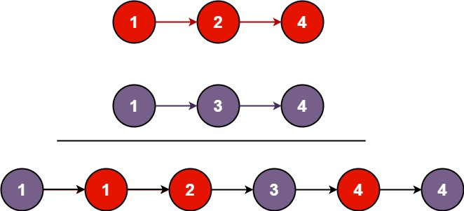
Input: list1 = [1,2,4], list2 = [1,3,4] Output: [1,1,2,3,4,4]
Example 2:
Input: list1 = [], list2 = [] Output: []
Example 3:
Input: list1 = [], list2 = [0] Output: [0]
Constraints:
- The number of nodes in both lists is in the range
[0, 50]. -100 <Node.val <= 100=- Both
list1andlist2are sorted in non-decreasing order.
※ 2.7.3.1. Constraints and Edge Cases
- empty lists inputs? – doesn’t seem like it needs to be explicitly handled though
※ 2.7.3.2. My Solution (Code)
※ 2.7.3.2.1. Wrong Attempt
1: # Definition for singly-linked list. 2: # class ListNode: 3: # def __init__(self, val=0, next=None): 4: # self.val = val 5: # self.next = next 6: class Solution: 7: │ def mergeTwoLists(self, list1: Optional[ListNode], list2: Optional[ListNode]) -> Optional[ListNode]: 8: │ │ if list1 and not list2: 9: │ │ │ return list1 10: │ │ if list2 and not list1: 11: │ │ │ return list2 12: │ │ if not list1 and not list2: 13: │ │ │ return None 14: │ │ │ 15: │ │ new_head = list1 if list1.val < list2.val else list2 16: │ │ p1, p2 = list1, list2 17: │ │ 18: │ │ # until one of them is None (used up) 19: │ │ while p1 != None and p2 != None: 20: │ │ │ if p1.val < p2.val: 21: │ │ │ │ tmp = p1.next 22: │ │ │ │ p1.next = tmp if tmp and tmp.val < p2.val else p2 23: │ │ │ │ p1 = tmp 24: │ │ │ else: 25: │ │ │ │ tmp = p2.next 26: │ │ │ │ p2.next = tmp if tmp and tmp.val < p1.val else p1 27: │ │ │ │ p2 = tmp 28: │ │ │ │ 29: │ │ return new_head 30:
Logic Flaw: Your approach tries to splice nodes in-place by switching next pointers based on value comparisons, but it doesn’t maintain a “builder” pointer to the merged list. This leads to broken chains or missed nodes, especially when the lists have interleaved values or different lengths.
※ 2.7.3.2.2. Optimal Solution
1: # Definition for singly-linked list. 2: # class ListNode: 3: # def __init__(self, val=0, next=None): 4: # self.val = val 5: # self.next = next 6: class Solution: 7: │ def mergeTwoLists(self, list1: Optional[ListNode], list2: Optional[ListNode]) -> Optional[ListNode]: 8: │ │ dummy = ListNode() 9: │ │ current = dummy 10: │ │ 11: │ │ # build up from current by using candidates from provider lists, list1 and list2 12: │ │ while list1 and list2: 13: │ │ │ if list1.val < list2.val: 14: │ │ │ │ current.next = list1 15: │ │ │ │ list1 = list1.next 16: │ │ │ else: 17: │ │ │ │ current.next = list2 18: │ │ │ │ list2 = list2.next 19: │ │ │ │ 20: │ │ │ # advance the builder pointer 21: │ │ │ current = current.next 22: │ │ │ 23: │ │ # Remnants: Attach the remaining part 24: │ │ current.next = list1 if list1 else list2 25: │ │ 26: │ │ return dummy.next
Complexity Analysis
- Time: \(O(n + m)\) worst case where each node is visited exactly once
- Space: \(O(1)\) since existing nodes used, nothing new used
Naming improvement suggestions:
- we can try using
tailinstead ofcurrentsince it’s the tail of the currently building linked list
Why dummy node? It simplifies head handling, so you never have to check if the merged list is empty.
this isn’t great for long lists because of the recursive depth:
1: def mergeTwoLists(self, l1, l2): 2: │ if not l1 or not l2: 3: │ │ return l1 or l2 4: │ if l1.val < l2.val: 5: │ │ l1.next = self.mergeTwoLists(l1.next, l2) 6: │ │ return l1 7: │ else: 8: │ │ l2.next = self.mergeTwoLists(l1, l2.next) 9: │ │ return l2 10:
the stack depth grows at \(O(n + m)\)
※ 2.7.3.3. My Approach/Explanation
※ 2.7.3.3.1. Initial, “wrong” mental model
I saw this as being a case where we have to “zip” together the two linked lists. This meant that I only had 2 pointers I was playing with. This works for some cases. It fails because we have either:
- no accumulator pointer that helps us “build” the newly accumulated linked lists
- OR no “previous” pointer of sorts that helps us with the remnants once we’re at the terminus
※ 2.7.3.3.2. Better Mental Model
We should see it as building a linked list (which is why we have a pointer to the last confirmed node) and we keep building to this. The current pointer may keep switching between the two lists as required.
This means that the other pointers pointing to the input lists are more like “providers” for candidates that will be considered.
Lastly, we just need to ensure that the remnant action is done. We can early-return for this.
※ 2.7.3.4. My Learnings/Questions
- Mental Model / Intuition for merging lists:
- Think of two “provider” pointers (list1, list2) and a “builder” pointer (current/tail) that constructs the merged list.
- Always attach the smaller node to the builder, advance the provider, and move the builder forward.
- When one provider runs out, attach the rest of the other list.
- TRICK: The dummy variable approach for the head() handling seems to be a really nifty trick Yes! It’s a classic way to handle head initialization for linked list problems, making code much cleaner.
QQ: I think strict inequalities are easier to reason with.
AA: For merging, yes. It’s common to use < so that equal elements are always taken from the same list (usually list2 in your code). This is fine and doesn’t affect correctness.
- We need a builder and we can’t slice things in place because that is error-prone
- Different approaches:
- Array-based Approach:
- You could convert both lists to arrays, merge them, and rebuild a new list, but this is not in-place and uses O(n+m) extra space—almost never the right choice for this problem.
- Priority Queue (Heap):
- Overkill for two lists, but useful for merging k sorted lists
- Array-based Approach:
※ 2.7.4. [36] Linked List Cycle (141) tortoise_hare_method
Given head, the head of a linked list, determine if the linked list
has a cycle in it.
There is a cycle in a linked list if there is some node in the list that
can be reached again by continuously following the next pointer.
Internally, pos is used to denote the index of the node
that tail’s next pointer is connected to. Note that pos is not
passed as a parameter.
Return true if there is a cycle in the linked list. Otherwise,
return false.
Example 1:
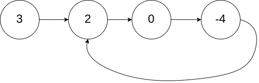
Input: head = [3,2,0,-4], pos = 1 Output: true Explanation: There is a cycle in the linked list, where the tail connects to the 1st node (0-indexed).
Example 2:
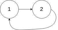
Input: head = [1,2], pos = 0 Output: true Explanation: There is a cycle in the linked list, where the tail connects to the 0th node.
Example 3:

Input: head = [1], pos = -1 Output: false Explanation: There is no cycle in the linked list.
Constraints:
- The number of the nodes in the list is in the range
[0, 10=^{=4}=]=. -10=^{=5}= <= Node.val <= 10=5posis-1or a valid index in the linked-list.
Follow up: Can you solve it using O(1) (i.e. constant) memory?
※ 2.7.4.1. Constraints and Edge Cases
- since it may be 0 nodes, we can do early returns by just checking for size = 0 or size = 1 which both trivially return as False
- classic edge cases:
- Handles empty list (head is None): returns False.
- Handles single node with no cycle: returns False.
- Handles cycle and no-cycle cases for longer lists.
※ 2.7.4.2. My Solution (Code)
1: # Definition for singly-linked list. 2: # class ListNode: 3: # def __init__(self, x): 4: # self.val = x 5: # self.next = None 6: 7: class Solution: 8: │ def hasCycle(self, head: Optional[ListNode]) -> bool: 9: │ │ # two independent pointers that hop on their own 10: │ │ slow, fast = head, head 11: │ │ if not slow or slow.next == None: 12: │ │ │ return False 13: │ │ │ 14: │ │ while True: 15: │ │ │ # if fast can't advance, then it's not a cycle anymore: 16: │ │ │ # make fast hop twice: 17: │ │ │ if not fast or not fast.next or not fast.next.next: 18: │ │ │ │ return False 19: │ │ │ │ 20: │ │ │ # make slow hop once: 21: │ │ │ if not slow or not slow.next: 22: │ │ │ │ return False 23: │ │ │ │ 24: │ │ │ fast = fast.next.next 25: │ │ │ slow = slow.next 26: │ │ │ 27: │ │ │ # has looped and returned 28: │ │ │ if fast == slow: 29: │ │ │ │ return True 30: │ │ │ │ 31: │ │ │ │ 32: │ │ # no need for fallthrough
- Minor style suggestions:
- You can simplify the loop by avoiding the
while Trueand instead usingwhile fast and fast.next. - You don’t need to check slow for
Noneinside the loop, since iffastandfast.nextare valid,slowwill always be valid.
- You can simplify the loop by avoiding the
※ 2.7.4.2.1. Canonical Style Optimal Solution
With the style suggestions above, here’s what we get:
1: class Solution: 2: │ def hasCycle(self, head: Optional[ListNode]) -> bool: 3: │ │ slow, fast = head, head 4: │ │ while fast and fast.next: 5: │ │ │ # if fast and fast.next are valid, they would have checked the previous nodes so slow will always be valid 6: │ │ │ slow = slow.next 7: │ │ │ fast = fast.next.next 8: │ │ │ if slow == fast: 9: │ │ │ │ return True 10: │ │ return False
※ 2.7.4.3. My Approach/Explanation
- We just run fast and slow pointers like the tortoise and hare style. If there’s a loop, the fast pointer will return and equal the slow one.
- careful: the order of state operations is important, the “check for equality” should be done AFTER the hopping based on this style of my implementation.
※ 2.7.4.4. My Learnings/Questions
- careful on when the equality check should be done. It’s intuitive to me if the equality checking should be done AFTER the hopping is done. The equality check is done after both pointers move, which is correct and avoids false positives at the start.
- This is the classic Floyd’s Tortoise and Hare (fast and slow pointer) algorithm see wikipedia page for other applications of this algo
- Style suggestions, intuition:
- if
fastandfast.nextare valid, they would have checked the previous nodes soslowwill always be valid
- if
※ 2.7.5. [37] Reorder List (143) in_place split_reverse_merge_method
You are given the head of a singly linked-list. The list can be represented as:
L0 → L1 → … → Ln - 1 → Ln
Reorder the list to be on the following form:
L0 → Ln → L1 → Ln - 1 → L2 → Ln - 2 → …
You may not modify the values in the list’s nodes. Only nodes themselves may be changed.
Example 1:

Input: head = [1,2,3,4] Output: [1,4,2,3]
Example 2:

Input: head = [1,2,3,4,5] Output: [1,5,2,4,3]
Constraints:
- The number of nodes in the list is in the range
[1, 5 * 10=^{=4}=]=. 1 <Node.val <= 1000=
※ 2.7.5.1. Constraints and Edge Cases
- need to prevent cycles because of the intermediate logic.
- even vs odd-lengthed lists should be handled well
- early return edge cases:
- 0, 1, or 2 nodes can just early return
※ 2.7.5.2. My Solution (Code)
※ 2.7.5.2.1. Optimal Solution \(O(n)\) time, \(O(1)\) space
- The optimal solution uses \(O(1)\) extra space by:
- Finding the middle of the list (slow/fast pointers).
- Reversing the second half of the list in-place.
- Merging the two halves by alternating nodes.
- Your Approach:
- Uses O(n) space for the stack, but is easier to implement and reason about.
1: class Solution: 2: │ def reorderList(self, head: Optional[ListNode]) -> None: 3: │ │ # early exits for the trivial edge cases: 4: │ │ if not head or not head.next: 5: │ │ │ return 6: │ │ │ 7: │ │ # Step 1: Find the middle 8: │ │ slow, fast = head, head 9: │ │ while fast and fast.next: 10: │ │ │ slow = slow.next 11: │ │ │ fast = fast.next.next 12: │ │ │ 13: │ │ # Step 2: Reverse the second half, slow is now at the middle 14: │ │ prev, curr = None, slow.next 15: │ │ slow.next = None # Split the list, now we have 2 lists 16: │ │ while curr: 17: │ │ │ next_temp = curr.next 18: │ │ │ curr.next = prev 19: │ │ │ prev = curr 20: │ │ │ curr = next_temp 21: │ │ │ 22: │ │ # Step 3: Merge two halves, this is like a ZIP operation 23: │ │ first, second = head, prev 24: │ │ while second: 25: │ │ │ tmp1, tmp2 = first.next, second.next 26: │ │ │ first.next = second 27: │ │ │ second.next = tmp1 28: │ │ │ first, second = tmp1, tmp2
※ 2.7.5.2.2. non-optimal Stack approach (more space usage)
Intuition: If you want to use a stack, push all nodes onto the stack, then for the first half, alternate popping from the stack and connecting nodes.
here’s the CORRECT way to do it using a stack:
1: class Solution: 2: │ def reorderList(self, head: Optional[ListNode]) -> None: 3: │ │ if not head or not head.next: 4: │ │ │ return 5: │ │ │ 6: │ │ # Push all nodes onto a stack 7: │ │ stack = [] 8: │ │ curr = head 9: │ │ while curr: 10: │ │ │ stack.append(curr) 11: │ │ │ curr = curr.next 12: │ │ │ 13: │ │ n = len(stack) 14: │ │ curr = head 15: │ │ for i in range(n // 2): 16: │ │ │ # Pop from the end 17: │ │ │ node = stack.pop() 18: │ │ │ node.next = curr.next 19: │ │ │ curr.next = node 20: │ │ │ curr = node.next 21: │ │ │ 22: │ │ # End the list 23: │ │ if curr: 24: │ │ │ curr.next = None
It doesn’t fare too well w.r.t the population.
Time and Space Complexity
- Time Complexity:
- O(n), where n is the number of nodes. Each node is visited at most twice (once to build the stack, once to relink).
- Space Complexity:
- O(n), since the stack stores up to n-1 nodes.
this was my first WRONG attempt and it has the following bugs (all pointer update bugs):
1: # Definition for singly-linked list. 2: # class ListNode: 3: # def __init__(self, val=0, next=None): 4: # self.val = val 5: # self.next = next 6: class Solution: 7: │ def reorderList(self, head: Optional[ListNode]) -> None: 8: │ │ """ 9: │ │ Do not return anything, modify head in-place instead. 10: │ │ """ 11: │ │ # init the right pointer: 12: │ │ left, right = head, head 13: │ │ # this will always be the right_next 14: │ │ stack = [] 15: │ │ while right.next: 16: │ │ │ stack.append(right) 17: │ │ │ right = right.next 18: │ │ │ 19: │ │ while stack and left != right: 20: │ │ │ left_next = left.next 21: │ │ │ right_next = stack.pop() 22: │ │ │ 23: │ │ │ left.next = right 24: │ │ │ right.next = left_next 25: │ │ │ left_next = right_next 26: │ │ │ 27: │ │ │ left = left_next 28: │ │ │ right = right_next 29: │ │ │ 30: │ │ left.next = None 31: │ │ 32: │ │ return
Here are the problems with this:
- since it’s not all the nodes in here, it makes the checks
You want to alternate between left and right, but your pointer updates are off. The main issue is with these lines:
Show/Hide Python Codeleft_next = left.next right_next = stack.pop() left.next = right right.next = left_next left_next = right_next left = left_next right = right_next
left_next = right_nextdoes nothing useful.- The advancing of
leftandrightis off.
Here’s how to maintain this style (of stack always containing one node before the right)
1: class Solution: 2: │ def reorderList(self, head: Optional[ListNode]) -> None: 3: │ │ if not head or not head.next: 4: │ │ │ return 5: │ │ │ 6: │ │ # Build stack of all nodes except the last one 7: │ │ stack = [] 8: │ │ curr = head 9: │ │ while curr.next: 10: │ │ │ stack.append(curr) 11: │ │ │ curr = curr.next 12: │ │ right = curr # The last node 13: │ │ 14: │ │ left = head 15: │ │ while stack and left != right and left.next != right: 16: │ │ │ # Get the previous node before right 17: │ │ │ prev = stack.pop() 18: │ │ │ # Save next node after left 19: │ │ │ left_next = left.next 20: │ │ │ 21: │ │ │ # Re-link nodes 22: │ │ │ left.next = right 23: │ │ │ right.next = left_next 24: │ │ │ 25: │ │ │ # Advance pointers 26: │ │ │ left = left_next 27: │ │ │ right = prev 28: │ │ │ 29: │ │ # Set the next of the last node to None to avoid cycles 30: │ │ right.next = None
Some observations from this:
- the while loop avoids cycles by including the AND clause of
left.next !=right - there’s some early returns that are well-handled
- the realisation that the last node will always be pointed at by the
rightpointer, so that’s the one we want to set toNone- How This Works
- The stack holds all nodes except the last (
right). - In each iteration:
- You link
left.nexttoright(the current last node). - Then,
right.nextto the next node after left (left_next). - Advance
leftto its next node (left_next). - Move
rightto the previous node (from the stack, it’s the top of stack).
- You link
- The loop stops when left meets or passes right.
- Finally, set
right.next = Noneto terminate the list.
- The stack holds all nodes except the last (
- How This Works
- Key Points
- Stack only contains the “rightnext” nodes (nodes before the last).
- No cycles: Always set the final node’s .next to None.
- Works for even and odd length lists.
※ 2.7.5.3. My Approach/Explanation
I had a stack-based implementation that was almost close. The idea was to keep history of visited on the stack, since finding the next from the right hand side is hard.
※ 2.7.5.4. My Learnings/Questions
- Observations / Intuition:
- we need to find the halfway point then do things as we need
- the stack approach uses extra space and hence is not ideal
So the intuition for the canonical solution: As shown above, the “split, reverse, merge” method is the canonical \(O(1)\) space solution.
Intuition for O(1) Space Solution: The order is: first node, last node, second node, second-last node, etc. By splitting and reversing, you can walk from both ends simultaneously without extra storage.
- seems like the main cause of bugs for me is really just the pointer update bugs.
- Careful on the return format expected by the question. In this case, the question just wants us to do the modifications and return nothing.
※ 2.7.6. [38] Remove Nth Node from End of List (19) med dummy_node_method
Given the head of a linked list, remove the n=^{=th} node from the
end of the list and return its head.
Example 1:
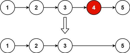
Input: head = [1,2,3,4,5], n = 2 Output: [1,2,3,5]
Example 2:
Input: head = [1], n = 1 Output: []
Example 3:
Input: head = [1,2], n = 1 Output: [1]
Constraints:
- The number of nodes in the list is
sz. 1 <sz <= 30=0 <Node.val <= 100=1 <n <= sz=
Follow up: Could you do this in one pass?
※ 2.7.6.1. Constraints and Edge Cases
- single size and
n =1=, then need to remove it. - empty list
- when head should be removed
※ 2.7.6.2. My Solution (Code)
※ 2.7.6.2.1. Optimal Solution
1: # Definition for singly-linked list. 2: # class ListNode: 3: # def __init__(self, val=0, next=None): 4: # self.val = val 5: # self.next = next 6: class Solution: 7: │ def removeNthFromEnd(self, head: Optional[ListNode], n: int) -> Optional[ListNode]: 8: │ │ dummy = ListNode(next=head) 9: │ │ slow, fast = dummy, dummy 10: │ │ 11: │ │ # move fast for fixed distance 12: │ │ for _ in range(n + 1): 13: │ │ │ fast = fast.next 14: │ │ │ 15: │ │ # move till the end: 16: │ │ while fast: 17: │ │ │ fast = fast.next 18: │ │ │ slow = slow.next 19: │ │ │ 20: │ │ # so the removal target the one after slow 21: │ │ # we have to join just adjacent 22: │ │ slow.next = slow.next.next 23: │ │ 24: │ │ return dummy.next
The main learning here is just how the dummy node helps to make things simpler.
- Complexity Analysis:
- Time Complexity: \(O(L)\), where \(L\) is the length of the list (one pass).
- Space Complexity: \(O(1)\), only a few pointers used.
※ 2.7.6.2.2. Failures
The Key Bug in my failed attempts were:
- Removing the head node (when
n =length of list=) is not handled correctly. [Edge case handling] - General pointer manipulation is off, especially when slow is just before the node to be removed.
First attempt was this:
1: # Definition for singly-linked list. 2: # class ListNode: 3: # def __init__(self, val=0, next=None): 4: # self.val = val 5: # self.next = next 6: class Solution: 7: │ def removeNthFromEnd(self, head: Optional[ListNode], n: int) -> Optional[ListNode]: 8: │ │ # trivial empty 9: │ │ if not head: 10: │ │ │ return head 11: │ │ │ 12: │ │ if n == 1 and not head.next: 13: │ │ │ return None 14: │ │ │ 15: │ │ # create the fixed distance: 16: │ │ slow, fast, fast_next = head, head, head 17: │ │ for _ in range(n): 18: │ │ │ if not fast_next.next: 19: │ │ │ │ return head 20: │ │ │ fast = fast.next 21: │ │ │ fast_next = fast_next.next 22: │ │ │ 23: │ │ while fast_next: 24: │ │ │ slow = slow.next 25: │ │ │ fast = fast.next 26: │ │ │ fast_next = fast_next.next 27: │ │ │ 28: │ │ target = slow.next 29: │ │ slow.next = fast 30: │ │ 31: │ │ return head
Here’s what’s wrong with this:
- Your pointer logic is off, and the special case handling is not robust.
- You use three pointers (
slow, fast, fast_next), but the way you advance them and check for the end is confusing and can miss the case where you need to remove the head node. - the for loop is problematic.
- This will return early if
fast_next.nextisNone, but if you need to remove the head (i.e.,n =length of list=), you should returnhead.next, nothead
- This will return early if
- You use three pointers (
Second attempt was this:
1: # Definition for singly-linked list. 2: # class ListNode: 3: # def __init__(self, val=0, next=None): 4: # self.val = val 5: # self.next = next 6: class Solution: 7: │ def removeNthFromEnd(self, head: Optional[ListNode], n: int) -> Optional[ListNode]: 8: │ │ # trivial cases: 9: │ │ # 1. empty 10: │ │ # attempt to create the space, we should be able to move n nodes 11: │ │ slow, fast = head, head 12: │ │ for _ in range(n): 13: │ │ │ if not fast.next: 14: │ │ │ │ return head 15: │ │ │ fast = fast.next 16: │ │ │ 17: │ │ while fast.next: 18: │ │ │ fast = fast.next 19: │ │ │ slow = slow.next 20: │ │ │ 21: │ │ slow.next = fast 22: │ │ 23: │ │ return head
- Issue:
- Similar pointer confusion.
- If
fast.nextisNoneduring the initial advance, you returnhead. But if you need to remove the head, you should returnhead.next.
- If
- Similar pointer confusion.
※ 2.7.6.3. My Approach/Explanation
I realise that I can borrow from the fast and slow pointer approach and create a fixed distance of size n.
If I can’t create the fixed distance, (means I encounter a None for the look-ahead, then I know that it’s not possible to cut things out so I need to just return the head without doing anything).
I wonder if a dummy node works well here. ⭐️ YES I SHOULD HAVE USED THIS.
※ 2.7.6.4. My Learnings/Questions
Optimal Solution: Intuition: The one-pass, two-pointer method is optimal for both time and space. Use a dummy node, advance fast n+1 steps, then move both pointers until fast is None. Remove slow.next.
Your Approach: Similar idea, but pointer logic and head-removal handling are off.
- Careful:
- the thing to remove was just a single node, not the whole section of nodes.
- Why dummy node? Handles the case where the head itself needs to be removed.
QQ: I suspect that it’s the trivial cases that are causing me to fail, the general case seems to be alright?
AA: Yes. Removing the head node (when n == length of list) is the main edge case. The dummy node pattern fixes this elegantly.
- alternative approaches:
Two-Pass Approach
First pass: Count the length of the list.
Second pass: Remove the \((L-n)^{th}\) node.
Time: \(O(L)\), but requires two passes.
Stack Approach
Push all nodes onto a stack, then pop n nodes, and relink.
Space: \(O(L)\), not optimal.
Array Approach
Convert to array, remove, rebuild list. Not recommended.
※ 2.7.6.5. [Optional] Additional Context
I struggled with this again and have issues with the clarity of thought. I’ll come back to this after doing a few other questions.
The fixed space distance and then running it along was the key idea as well, I am happy I got it.
※ 2.7.7. [39] Copy List with Random Pointer (138) interleaving_method
A linked list of length n is given such that each node contains an
additional random pointer, which could point to any node in the list, or
null.
Construct a
deep copy
of the list. The deep copy should consist of exactly n brand new
nodes, where each new node has its value set to the value of its
corresponding original node. Both the next and random pointer of the
new nodes should point to new nodes in the copied list such that the
pointers in the original list and copied list represent the same list
state. None of the pointers in the new list should point to nodes in
the original list.
For example, if there are two nodes X and Y in the original list,
where X.random --> Y, then for the corresponding two nodes x and y
in the copied list, x.random --> y.
Return the head of the copied linked list.
The linked list is represented in the input/output as a list of n
nodes. Each node is represented as a pair of [val, random_index]
where:
val: an integer representingNode.valrandom_index: the index of the node (range from0ton-1) that therandompointer points to, ornullif it does not point to any node.
Your code will only be given the head of the original linked list.
Example 1:
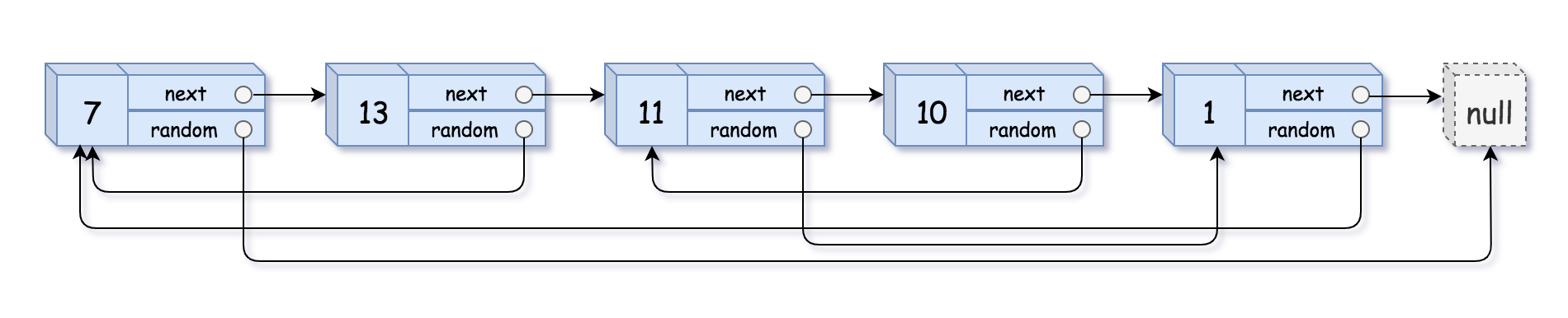
Input: head = [[7,null],[13,0],[11,4],[10,2],[1,0]] Output: [[7,null],[13,0],[11,4],[10,2],[1,0]]
Example 2:

Input: head = [[1,1],[2,1]] Output: [[1,1],[2,1]]
Example 3:

Input: head = [[3,null],[3,0],[3,null]] Output: [[3,null],[3,0],[3,null]]
Constraints:
0 <n <= 1000=-10=^{=4}= <= Node.val <= 10=4Node.randomisnullor is pointing to some node in the linked list.
※ 2.7.7.1. Constraints and Edge Cases
- had to early-return the empty linked list case
※ 2.7.7.2. My Solution (Code)
This is the most optimal solution!
1: """ 2: # Definition for a Node. 3: class Node: 4: │ def __init__(self, x: int, next: 'Node' = None, random: 'Node' = None): 5: │ self.val = int(x) 6: │ self.next = next 7: │ self.random = random 8: """ 9: 10: class Solution: 11: │ def copyRandomList(self, head: 'Optional[Node]') -> 'Optional[Node]': 12: │ │ if not head: 13: │ │ │ return None 14: │ │ # single list, with the new duplicates as well 15: │ │ # this forms the following: O1-> N1 -> O2 -> N2 -> O3 -> N3 -> ... -> ON -> NN 16: │ │ old = head 17: │ │ while old: 18: │ │ │ new = ListNode(val=old.val, next=old.next) 19: │ │ │ old.next = new 20: │ │ │ old = new.next 21: │ │ │ 22: │ │ # we correct the assignments on the new guys to be 1 away: 23: │ │ old = head 24: │ │ while old: 25: │ │ │ new = old.next 26: │ │ │ old_random_target = old.random 27: │ │ │ new_random_target = old.random.next if old.random else None 28: │ │ │ new.random = new_random_target 29: │ │ │ old = new.next 30: │ │ │ 31: │ │ # now we split the merged list into old and new lists: 32: │ │ old = head 33: │ │ new = new_head = old.next 34: │ │ while new: 35: │ │ │ next_old = new.next 36: │ │ │ next_new = new.next.next if new.next else None 37: │ │ │ new.next = next_new 38: │ │ │ new = next_new 39: │ │ │ old = next_old 40: │ │ │ 41: │ │ return new_head
This has a \(O(n)\) time, \(O(1)\) space, three passes approach.
A little cleaner of an implementation is:
1: class Solution: 2: │ def copyRandomList(self, head: 'Optional[Node]') -> 'Optional[Node]': 3: │ │ if not head: 4: │ │ │ return None 5: │ │ │ 6: │ │ # 1. Interleave copied nodes with originals 7: │ │ curr = head 8: │ │ while curr: 9: │ │ │ copy = Node(curr.val, curr.next) 10: │ │ │ curr.next = copy 11: │ │ │ curr = copy.next 12: │ │ │ 13: │ │ # 2. Assign random pointers for the copied nodes 14: │ │ curr = head 15: │ │ while curr: 16: │ │ │ copy = curr.next 17: │ │ │ copy.random = curr.random.next if curr.random else None 18: │ │ │ curr = copy.next 19: │ │ │ 20: │ │ # 3. Separate the original and copied lists 21: │ │ curr = head 22: │ │ copy_head = head.next 23: │ │ while curr: 24: │ │ │ copy = curr.next 25: │ │ │ curr.next = copy.next 26: │ │ │ copy.next = copy.next.next if copy.next else None 27: │ │ │ curr = curr.next 28: │ │ │ 29: │ │ return copy_head
※ 2.7.7.2.1. Alternative (space-wasting) hashmap solution
This works with the same \(O(n)\) runtime but with \(O(n)\) space instead of \(O(1)\).
The concept is similar, we want to keep a mapping between old and new versions so that we can make references to who they were linked to.
1: class Solution: 2: │ def copyRandomList(self, head: 'Optional[Node]') -> 'Optional[Node]': 3: │ │ if not head: 4: │ │ │ return None 5: │ │ old_to_new = {} 6: │ │ curr = head 7: │ │ while curr: 8: │ │ │ old_to_new[curr] = Node(curr.val) 9: │ │ │ curr = curr.next 10: │ │ curr = head 11: │ │ while curr: 12: │ │ │ old_to_new[curr].next = old_to_new.get(curr.next) 13: │ │ │ old_to_new[curr].random = old_to_new.get(curr.random) 14: │ │ │ curr = curr.next 15: │ │ return old_to_new[head]
※ 2.7.7.3. My Approach/Explanation
The key intuition in my approach is:
We want to be able to do manipulations without destroying relationships, and we want to handle them simultaneously.
We can describe the explicit pointers to be explicit relationships between a node and another.
This means that we can introduce implicit relationships in addition to these explicit relationships.
We can merge old and new and let their relative ordering hold implicit meaning for us.
- So if we merge in an interleaved fashion such that we get \({\{O1, N1, O2, N2, O3, N3,..., O_{N-1}, N_{N-1}, O_{N}, N_{N}\}}\), where \(O_{i}\) is the ${ith} node from original list and \(N_{i}\) is its corresponding new node, then we can keep all of:
- existing
nextrelationships (implicit, requires double jumping) - existing
randomrelationships (explicit ones)
- existing
- so the 3 passes would be:
- merge the old and new list, interleave old and new
- correct the assignments for new news to do the double hops
- correct the random pointer assignments for new nodes using double hops from the old ones
※ 2.7.7.4. My Learnings/Questions
- my intuition here is great
- I think I boiled a linked list down to the mathematical foundations of relations and then defined them as implicit or explicit relations. The Explicit ones could be made implicit / transitive and that was the main spark.
- Careful on the double-jumps, they need to have
Nonesentinels just in case since the double jump could actually be aNonevalue
※ 2.7.7.5. Additional Context
I’m really happy with this one. It’s actually the optimal method 🎉
※ 2.7.8. [40] Add two numbers (2) dummy_node_method human_calculation
You are given two non-empty linked lists representing two non-negative integers. The digits are stored in reverse order, and each of their nodes contains a single digit. Add the two numbers and return the sum as a linked list.
You may assume the two numbers do not contain any leading zero, except the number 0 itself.
Example 1:
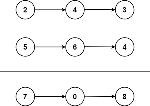
Input: l1 = [2,4,3], l2 = [5,6,4] Output: [7,0,8] Explanation: 342 + 465 = 807.
Example 2:
Input: l1 = [0], l2 = [0] Output: [0]
Example 3:
Input: l1 = [9,9,9,9,9,9,9], l2 = [9,9,9,9] Output: [8,9,9,9,0,0,0,1]
Constraints:
- The number of nodes in each linked list is in the range
[1, 100]. 0 <Node.val <= 9=- It is guaranteed that the list represents a number that does not have leading zeros.
※ 2.7.8.1. Constraints and Edge Cases
- it’s mainly numeric / human number addition edge cases to handle:
- even if one of the input “number”s have been read fully, we can still have cases where there’s a cascade of carry operations that modify every single digit for the remaining “number”. For example if
carry = 1and we haveremaining digits = {9,9,9,9,9}- for this, before returning, we check for remnant carry and add a new node to the builder
- even if one of the input “number”s have been read fully, we can still have cases where there’s a cascade of carry operations that modify every single digit for the remaining “number”. For example if
- Your solution is mostly correct and handles the main cases:
- Adds corresponding digits from both lists.
- Handles carry propagation.
- Correctly attaches remaining nodes from the longer list and continues carry propagation.
- Appends a new node if there is a final carry.
- if we are using one of the existing linked lists as the results list, then we’d need to
※ 2.7.8.2. My Solution (Code)
My solution feels fast but there’s likely a cleaner way to write it.
1: # Definition for singly-linked list. 2: # class ListNode: 3: # def __init__(self, val=0, next=None): 4: # self.val = val 5: # self.next = next 6: class Solution: 7: │ def addTwoNumbers(self, l1: Optional[ListNode], l2: Optional[ListNode]) -> Optional[ListNode]: 8: │ │ # builder is somewhat of a lookback dummy 9: │ │ first, second, builder = l1, l2, ListNode(next=l1) 10: │ │ carry = 0 11: │ │ 12: │ │ # no need for dummy, it's guaranteed to have one 13: │ │ # use first list for the answer 14: │ │ while first and second: 15: │ │ │ res = carry 16: │ │ │ res += first.val + second.val 17: │ │ │ carry, res_digit = divmod(res, 10) 18: │ │ │ # assign: 19: │ │ │ first.val = res_digit 20: │ │ │ 21: │ │ │ builder = first 22: │ │ │ first = first.next 23: │ │ │ second = second.next 24: │ │ │ 25: │ │ │ 26: │ │ # carrying still needs to be done 27: │ │ if not first and second: 28: │ │ │ while second: 29: │ │ │ │ builder.next = second 30: │ │ │ │ res = second.val + carry 31: │ │ │ │ carry, res_digit = divmod(res, 10) 32: │ │ │ │ second.val = res_digit 33: │ │ │ │ builder = builder.next 34: │ │ │ │ second = second.next 35: │ │ │ │ # early return if no extra carries to handle 36: │ │ │ │ if carry == 0: 37: │ │ │ │ │ break 38: │ │ if not second and first: 39: │ │ │ while first: 40: │ │ │ │ builder.next = first 41: │ │ │ │ res = first.val + carry 42: │ │ │ │ carry, res_digit = divmod(res, 10) 43: │ │ │ │ first.val = res_digit 44: │ │ │ │ builder = builder.next 45: │ │ │ │ first = first.next 46: │ │ │ │ # early return if no extra carries to handle 47: │ │ │ │ if carry == 0: 48: │ │ │ │ │ break 49: │ │ │ │ │ 50: │ │ # last check if still have carry: 51: │ │ if carry: 52: │ │ │ builder.next = ListNode(val=carry) 53: │ │ │ 54: │ │ return l1
- Time Complexity:
- \(O(max(m, n))\), where \(m\) and \(n\) are the lengths of the two lists. Each node is visited once.
- Space Complexity:
- \(O(1)\) extra space (not counting the output list), since you reuse existing nodes and only allocate a new node for a final carry.
※ 2.7.8.2.1. More idiomatic implementation, with result linked list built out
Uses a dummy node and a single loop, always creating new nodes for the result list. This is more robust and idiomatic.
1: class Solution: 2: │ def addTwoNumbers(self, l1: Optional[ListNode], l2: Optional[ListNode]) -> Optional[ListNode]: 3: │ │ dummy = ListNode() 4: │ │ tail = dummy 5: │ │ carry = 0 6: │ │ 7: │ │ p1, p2 = l1, l2 8: │ │ while p1 or p2 or carry: 9: │ │ │ val1 = p1.val if p1 else 0 10: │ │ │ val2 = p2.val if p2 else 0 11: │ │ │ total = val1 + val2 + carry 12: │ │ │ carry, digit = divmod(total, 10) 13: │ │ │ tail.next = ListNode(digit) 14: │ │ │ tail = tail.next 15: │ │ │ 16: │ │ │ if p1: p1 = p1.next 17: │ │ │ if p2: p2 = p2.next 18: │ │ │ 19: │ │ return dummy.next 20:
- Uses a single loop that continues as long as at least one of the input lists has nodes or there’s a carry.
Advantages:
- Never mutates input lists.
- Handles all edge cases (different lengths, final carry) in a single loop.
- Clean and easy to maintain.
※ 2.7.8.3. My Approach/Explanation
This is a typical human-like addition algorithm that we need to do using linked lists. Off the bat, we know:
- the carrying needs to be handled well
- since it’s all using linked lists, as long as we don’t lose the pointers, we can just re-use the existing linked list nodes for our answer without incuring any extra space usage.
Here, I choose to have a lookback pointer (builder) that points at the most recently added answer list, this helps us reuse the nodes.
※ 2.7.8.4. My Learnings/Questions
- the bot got upset I reused the input list and modified it. In the real world, I would have clarified if this was the case. Since it was not explicitly guarded against by the question, I shall take it as fair game and I shall treat mine as superior.
- it’s nice that I have the intuition for the dummy pointer / builder pointer being used as a lookback pointer. I like this.
- the
divmodis amazing - extensions / alternative approaches:
- Convert to Integers:
- Convert both lists to integers, add, then convert back to a list.
- Drawback: Not suitable for very large numbers (beyond Python’s int).
- Stack Approach:
- For numbers stored in forward order (not this problem), you might use stacks to process from least to most significant digit.
- Recursive Approach:
- For numbers stored in forward order, recursion can help align the lists.
※ 2.7.8.5. Additional Context
I got this right first time! Confidence boosted 🚀
※ 2.7.9. [41] ⭐️ Find the Duplicate Number (287) redo tortoise_hare_method array linked_list
Given an array of integers nums containing n + 1 integers where each
integer is in the range [1, n] inclusive.
There is only one repeated number in nums, return
this repeated number.
You must solve the problem without modifying the array nums and
using only constant extra space.
Example 1:
Input: nums = [1,3,4,2,2] Output: 2
Example 2:
Input: nums = [3,1,3,4,2] Output: 3
Example 3:
Input: nums = [3,3,3,3,3] Output: 3
Constraints:
1 <n <= 10=5nums.length =n + 1=1 <nums[i] <= n=- All the integers in
numsappear only once except for precisely one integer which appears two or more times.
Follow up:
- How can we prove that at least one duplicate number must exist in
nums? - Can you solve the problem in linear runtime complexity?
※ 2.7.9.1. Constraints and Edge Cases
No modification of nums and only using extra space.
※ 2.7.9.2. My Solution (Code)
※ 2.7.9.2.1. Optimal Floyd’s Tortoise and Hare Method (Cycle Detection + Creator Detection in most efficient (\(O(n)\) time, \(O(1)\) space))
Key Insights
- See Array as a linked list: because of the \(n + 1\) integers in the range \([1, n]\), we can use the list like a linked list. We can choose \(nums[i]\) to be the “next” pointer.
- this works for us, if there’s a duplicate, we’d end up again at that “node” –> tortoise and hare method
- We will do things in 2 phases:
- phase 1: find the intersection point
- Use two pointers (slow and fast).
- Move slow by 1 step, fast by 2 steps.
- They will meet inside the cycle.
- phase 2: find the entrance to the cycle
- Reset one pointer to the start.
- Move both pointers by 1 step.
- The node where they meet is the duplicate.
- phase 1: find the intersection point
- The intersection point of the cycle is where the faster-moving hare meets the slower-moving tortoise this is the reason we can run phase 2 like we did, we essentially just re-do the shifting but at the same speed.
1: class Solution: 2: │ def findDuplicate(self, nums: List[int]) -> int: 3: │ │ # Phase 1: Find intersection 4: │ │ slow = fast = nums[0] 5: │ │ while True: 6: │ │ │ slow = nums[slow] 7: │ │ │ fast = nums[nums[fast]] # double jump 8: │ │ │ if slow == fast: 9: │ │ │ │ break 10: │ │ │ │ 11: │ │ # Phase 2: Find entrance to the cycle 12: │ │ fast = nums[0] # reset to beginning 13: │ │ while slow != fast: 14: │ │ │ slow = nums[slow] 15: │ │ │ fast = nums[fast] 16: │ │ return slow
※ 2.7.9.2.2. Inferior binary search solution
- Key idea: The numbers are in the range \([1, n]\). Use binary search on this range.
- How it works:
- For a guess
mid, count how many numbers in nums are <= mid. - If the count is > mid, the duplicate is in \([1, mid]\).
- Otherwise, it’s in \([mid+1, n]\).
- Repeat until you find the duplicate.
- For a guess
- Why does this work?
- If there were no duplicates, count of \(numbers ≤ mid\) would be at most mid.
- If there are more, the duplicate must be in that range.
It’s slower
1: class Solution: 2: │ def findDuplicate(self, nums: List[int]) -> int: 3: │ │ left, right = 1, len(nums) - 1 4: │ │ while left < right: 5: │ │ │ mid = (left + right) // 2 6: │ │ │ count = sum(num <= mid for num in nums) 7: │ │ │ if count > mid: 8: │ │ │ │ right = mid 9: │ │ │ else: 10: │ │ │ │ left = mid + 1 11: │ │ return left
Why does the binary search work? The “pigeonhole principle”: more numbers ≤ mid than mid itself means the duplicate is in that range.
※ 2.7.9.3. My Approach/Explanation
The slower approach of using binary search on the value range is something that I also thought of initially. Since we know the range of the numbers we can binary search it. For each iteration, we just need to sweep through the nums array and check if that’s the duplicate (can use a int counter for this).
As for the actual solution, This one was the entire floyd’s tortoise and hare algorithm used properly. What we need to do here is that we know there’s going to be a “cycle”, but we need to do another step which is to find where the cycle gets created.
※ 2.7.9.4. My Learnings/Questions
- Key Intuition
- Each index is a “node,” and nums[i] is a “next” pointer.
- The duplicate number creates a cycle in this “linked list.”
- Floyd’s algorithm finds the cycle’s entry, which is the duplicate.
- the way to see the array as a linked list is one of the most important realisations here, it’s because of the constraints given to us.
- turns out that floyd’s algo can be used for both cycle detection AND finding the cycle creator.
- All the great stuff about floyd’s tortoise and hare algorithm!
- the inferior (binary search method) works because of the pigeonhole principle
※ 2.7.9.5. [Optional] Additional Context
<e.g., “I struggled with X”, “I want to know about alternative algorithms”, etc.>
This is a non-obvious trick
※ 2.7.10. [42] LRU Cache (146)
Design a data structure that follows the constraints of a Least Recently Used (LRU) cache.
Implement the LRUCache class:
LRUCache(int capacity)Initialize the LRU cache with positive sizecapacity.int get(int key)Return the value of thekeyif the key exists, otherwise return-1.void put(int key, int value)Update the value of thekeyif thekeyexists. Otherwise, add thekey-valuepair to the cache. If the number of keys exceeds thecapacityfrom this operation, evict the least recently used key.
The functions get and put must each run in O(1) average time
complexity.
Example 1:
Input
["LRUCache", "put", "put", "get", "put", "get", "put", "get", "get", "get"]
[[2], [1, 1], [2, 2], [1], [3, 3], [2], [4, 4], [1], [3], [4]]
Output
[null, null, null, 1, null, -1, null, -1, 3, 4]
Explanation
LRUCache lRUCache = new LRUCache(2);
lRUCache.put(1, 1); // cache is {1=1}
lRUCache.put(2, 2); // cache is {1=1, 2=2}
lRUCache.get(1); // return 1
lRUCache.put(3, 3); // LRU key was 2, evicts key 2, cache is {1=1, 3=3}
lRUCache.get(2); // returns -1 (not found)
lRUCache.put(4, 4); // LRU key was 1, evicts key 1, cache is {4=4, 3=3}
lRUCache.get(1); // return -1 (not found)
lRUCache.get(3); // return 3
lRUCache.get(4); // return 4
Constraints:
1 <capacity <= 3000=0 <key <= 10=40 <value <= 10=5- At most
2 * 10=^{=5} calls will be made togetandput.
※ 2.7.10.1. Constraints and Edge Cases
<list constraints, input limits, or tricky edge cases here>
※ 2.7.10.2. My Solution (Code)
※ 2.7.10.2.1. Optimal Solution
this is actually the “underthehood” for the OrderedDict implementation.
We need to keep track of:
- relative ordering of things via a linked list (doubly) and a hashmap
- jump map as a reference to the nodes we need to jump to
1: class Node: 2: │ def __init__(self, key, val): 3: │ │ self.key = key 4: │ │ self.val = val 5: │ │ self.prev = self.next = None 6: │ │ 7: class LRUCache: 8: │ def __init__(self, capacity: int): 9: │ │ self.capacity = capacity 10: │ │ self.cache = {} # key -> node 11: │ │ # Dummy head and tail nodes 12: │ │ self.head, self.tail = Node(0, 0), Node(0, 0) 13: │ │ self.head.next, self.tail.prev = self.tail, self.head 14: │ │ 15: │ def _remove(self, node): 16: │ │ prev, nxt = node.prev, node.next 17: │ │ prev.next, nxt.prev = nxt, prev 18: │ │ 19: │ def _add(self, node): 20: │ │ prev, nxt = self.tail.prev, self.tail 21: │ │ prev.next = nxt.prev = node 22: │ │ node.prev, node.next = prev, nxt 23: │ │ 24: │ def get(self, key: int) -> int: 25: │ │ if key not in self.cache: 26: │ │ │ return -1 27: │ │ node = self.cache[key] 28: │ │ self._remove(node) 29: │ │ self._add(node) 30: │ │ return node.val 31: │ │ 32: │ def put(self, key: int, value: int) -> None: 33: │ │ if key in self.cache: 34: │ │ │ self._remove(self.cache[key]) 35: │ │ node = Node(key, value) 36: │ │ self.cache[key] = node 37: │ │ self._add(node) 38: │ │ if len(self.cache) > self.capacity: 39: │ │ │ # Remove from head 40: │ │ │ lru = self.head.next 41: │ │ │ self._remove(lru) 42: │ │ │ del self.cache[lru.key]
※ 2.7.10.2.2. pythonic “Cheat”: using OrderedDict
1: from collections import OrderedDict 2: class LRUCache: 3: │ 4: │ def __init__(self, capacity: int): 5: │ │ self.store = OrderedDict() 6: │ │ self.max = capacity 7: │ │ self.cap = 0 8: │ │ 9: │ def get(self, key: int) -> int: 10: │ │ if key not in self.store: 11: │ │ │ return -1 12: │ │ │ 13: │ │ # register as used: 14: │ │ self.store.move_to_end(key) 15: │ │ return self.store[key] 16: │ │ 17: │ │ 18: │ def put(self, key: int, value: int) -> None: 19: │ │ # shift usage if pre-existing: 20: │ │ if key in self.store: 21: │ │ │ self.store.move_to_end(key) 22: │ │ │ 23: │ │ self.store[key] = value 24: │ │ if (len(self.store) > self.max): 25: │ │ │ # evicts LRU item: 26: │ │ │ self.store.popitem(last=False) 27: │ │ │ 28: │ │ │ 29: │ │ │ 30: # Your LRUCache object will be instantiated and called as such: 31: # obj = LRUCache(capacity) 32: # param_1 = obj.get(key) 33: # obj.put(key,value)
To update the freshness, use move_to_end().
To pop LRU, use popitem(last=False)
※ 2.7.10.3. My Approach/Explanation
Kinda “cheated” here by using python’s OrderedDict.
※ 2.7.10.4. My Learnings/Questions
- Intuition:
- Hash map provides \(O(1)\) access.
- Doubly linked list (or OrderedDict) provides \(O(1)\) reordering and eviction.
we can use OrderedDict for both LRU cache and MRU cache:
for the eviction, modulate the
popitem(last=<param>)- if
last = True: then pairs are returned in LIFO order \(\implies\) MRU - if
last = False: then pairs are returned in FIFO order \(\implies\) LRU
- if
- single linked list will not have \(O(1)\) eviction, it will end up being \(O(n)\) because you’d need to traverse
※ 2.7.10.5. Additional Context
I had the intuition for the doubly linked list + hashmap correctly. First it’s about the time-based relationship (which is adequately represented by a linked list here).
Then we face 2 problems:
- how to jump to the correct node without traversing the whole list?
- how to go back from node to prev node?
※ 2.7.11. [43] Merge k sorted lists [23] hard merge_sort_merge_method min_heap
You are given an array of k linked-lists lists, each linked-list is
sorted in ascending order.
Merge all the linked-lists into one sorted linked-list and return it.
Example 1:
Input: lists = [[1,4,5],[1,3,4],[2,6]] Output: [1,1,2,3,4,4,5,6] Explanation: The linked-lists are: [ 1->4->5, 1->3->4, 2->6 ] merging them into one sorted linked list: 1->1->2->3->4->4->5->6
Example 2:
Input: lists = [] Output: []
Example 3:
Input: lists = [[]] Output: []
Constraints:
k =lists.length=0 <k <= 10=40 <lists[i].length <= 500=-10=^{=4}= <= lists[i][j] <= 10=4lists[i]is sorted in ascending order.- The sum of
lists[i].lengthwill not exceed10=^{=4}.
※ 2.7.11.1. Constraints and Edge Cases
- careful on the duplicate values, a tie-breaker is needed for python heapq for tuple comparisons
- empty lists to be handled
※ 2.7.11.2. My Solution (Code)
※ 2.7.11.2.1. Optimal, Using Min-Heap from heapq (\(O(N\log k)\) time, \(O(k)\) space)
This is the simplest to me, most pythonic
1: import heapq 2: 3: # Definition for singly-linked list. 4: # class ListNode: 5: # def __init__(self, val=0, next=None): 6: # self.val = val 7: # self.next = next 8: class Solution: 9: │ def mergeKLists(self, lists: List[Optional[ListNode]]) -> Optional[ListNode]: 10: │ │ # filters away the empty lists: 11: │ │ # NOTE: the use of id(ls) is to give a tie-breaker in the case that two lists have the same value. 12: │ │ # this id usage is an easy way to avoid compiler issues 13: │ │ providers = [(ls.val, id(ls), ls) 14: │ │ │ │ │ │for ls in lists 15: │ │ │ │ │ │if ls] 16: │ │ heapq.heapify(providers) 17: │ │ pre_head = dummy = ListNode() 18: │ │ 19: │ │ while providers: 20: │ │ │ (val, _, ls) = heapq.heappop(providers) 21: │ │ │ dummy.next = ls 22: │ │ │ if ls.next: 23: │ │ │ │ ls = ls.next 24: │ │ │ │ new_val = ls.val 25: │ │ │ │ heapq.heappush(providers, (new_val, id(ls), ls)) 26: │ │ │ │ 27: │ │ │ dummy = dummy.next 28: │ │ │ 29: │ │ return pre_head.next
- Complexity Analysis
- Time Complexity:
- Each of the total \(N\) nodes (sum of all nodes in all lists) is pushed and popped from the heap once.
- Heap size is at most \(k\) at any time.
- Total time: \(O(N \log k)\), where \(N\) is the total number of nodes.
- Space Complexity:
- The heap stores up to \(k\) elements: \(O(k)\).
- The output list uses \(O(N)\) space, but this is required for the result and not considered extra space.
- Time Complexity:
- the listcomp handles the empty list filtering as well.
※ 2.7.11.2.2. Optimal, Divide and Conquer (\(O(N\log k)\) time, \(O(1)\) space)
this does 2-pair list merges logarithmically. It’s like the merging step in mergesort.
Time Complexity: \(O(N\log k)\)
Space Complexity: \(O(1)\) (excluding output), as merging two lists is done in-place.
1: class Solution: 2: │ def mergeKLists(self, lists: List[Optional[ListNode]]) -> Optional[ListNode]: 3: │ │ if not lists: 4: │ │ │ return None 5: │ │ n = len(lists) 6: │ │ interval = 1 7: │ │ while interval < n: 8: │ │ │ for i in range(0, n - interval, interval * 2): 9: │ │ │ │ lists[i] = self.merge2Lists(lists[i], lists[i + interval]) 10: │ │ │ interval *= 2 11: │ │ return lists[0] if n > 0 else None 12: │ │ 13: │ def merge2Lists(self, l1, l2): 14: │ │ dummy = curr = ListNode() 15: │ │ while l1 and l2: 16: │ │ │ if l1.val < l2.val: 17: │ │ │ │ curr.next, l1 = l1, l1.next 18: │ │ │ else: 19: │ │ │ │ curr.next, l2 = l2, l2.next 20: │ │ │ # advance 21: │ │ │ curr = curr.next 22: │ │ │ 23: │ │ curr.next = l1 or l2 24: │ │ 25: │ │ return dummy.next 26:
※ 2.7.11.3. My Approach/Explanation
The pythonic way should be a little easier.
We have k lists and they are all providers.
We just need to keep a priority queue based on the value of the head of each provider each time (for which we can use python’s heapq) and then
※ 2.7.11.4. My Learnings/Questions
Main Intuition:
The heap approach is optimal because at any time, you only need to consider the smallest head node among
klists.Divide and conquer is optimal because merging two sorted lists is linear, and you reduce the number of lists logarithmically.
heapqhas a bunch of caveats:if there’s a tie, it needs a tie-breaker. If we don’t provide this, then it will try to use default comparators for the class, which in this case, will likely not be implemented, and that’s why we can have errors:
Why use id() as a tie-breaker?
In some cases (like merging k sorted linked lists), you may have multiple nodes with the same value.
If you push tuples like (node.val, node) to the heap, and two nodes have the same value, Python will try to compare the ListNode objects to break the tie.
If ListNode does not implement comparison methods, this will raise a TypeError because Python doesn’t know how to compare your custom objects
By using id(ls) as the second element, you guarantee uniqueness (since id() returns the memory address of the object), and Python can always compare integers, so the heap operations will never fail due to unorderable type
heapqcan’t heapify generators, has to be list
- the providers and builder analogy has been serving me well so far!
- the main other alternative is to use the merge sort’s merging approach, where we bottom-up merge a bunch of lists together
- other alternatives:
Brute Force
Collect all values, sort, and rebuild the list.
Time: \(O(N \log N)\)
Space: \(O(N)\)
Not optimal.
Divide and Conquer
As shown above, merge pairs of lists recursively/logarithmically.
Time: \(O(N \log k)\)
Space: \(O(1)\) extra (besides output).
Custom Min-Heap Implementation
Instead of Python’s heapq, you could implement your own min-heap, but this is unnecessary in Python.
※ 2.7.11.5. [Optional] Additional Context
<e.g., “I struggled with X”, “I want to know about alternative algorithms”, etc.>
※ 2.7.12. [44] Reverse nodes in k-Group (25) redo almost hard dummy_node_method sliding_window
Given the head of a linked list, reverse the nodes of the list k at
a time, and return the modified list.
k is a positive integer and is less than or equal to the length of the
linked list. If the number of nodes is not a multiple of k then
left-out nodes, in the end, should remain as it is.
You may not alter the values in the list’s nodes, only nodes themselves may be changed.
Example 1:
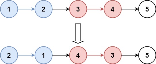
Input: head = [1,2,3,4,5], k = 2 Output: [2,1,4,3,5]
Example 2:
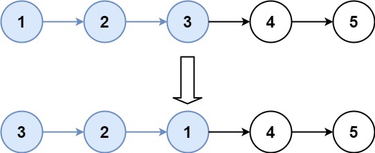
Input: head = [1,2,3,4,5], k = 3 Output: [3,2,1,4,5]
Constraints:
- The number of nodes in the list is
n. 1 <k <= n <= 5000=0 <Node.val <= 1000=
Follow-up: Can you solve the problem in O(1) extra memory space?
※ 2.7.12.1. Constraints and Edge Cases
Nothing fancy here
※ 2.7.12.2. My Solution (Code)
※ 2.7.12.2.1. Optimal, My initial version (needed corrections)
Initial approach, it’s incorrect but has the correct approach.
1: # Definition for singly-linked list. 2: # class ListNode: 3: # def __init__(self, val=0, next=None): 4: # self.val = val 5: # self.next = next 6: class Solution: 7: │ 8: │ # reverse all from left.next to right and then join that up with next 9: │ # also advance the pointers 10: │ def reverse(self, left, right, nxt): 11: │ │ dummy = left 12: │ │ prev , curr = None, left.next 13: │ │ 14: │ │ while curr != nxt: 15: │ │ │ right_ptr = curr.next 16: │ │ │ curr.next = prev 17: │ │ │ prev = curr 18: │ │ │ curr = right_ptr 19: │ │ │ 20: │ │ # so prev is the start that works 21: │ │ left.next = prev 22: │ │ # right next is nxt 23: │ │ right.next = nxt 24: │ │ 25: │ │ return left, right , nxt 26: │ │ 27: │ def reverseKGroup(self, head: Optional[ListNode], k: int) -> Optional[ListNode]: 28: │ │ # trivial edge cases 29: │ │ if not head or not head.next: 30: │ │ │ return head 31: │ │ │ 32: │ │ pre_head = left = right = ListNode(next=head) 33: │ │ nxt = right.next # starts at head 34: │ │ 35: │ │ while nxt: 36: │ │ │ # expand till we get window size k, if not just return whatever has been built 37: │ │ │ for _ in range(k): 38: │ │ │ │ nxt = nxt.next 39: │ │ │ │ if not nxt: 40: │ │ │ │ │ return pre_head.next 41: │ │ │ │ else: 42: │ │ │ │ │ right = right.next 43: │ │ │ │ │ 44: │ │ │ # window of size k exists now, it's from left -..-> right 45: │ │ │ left, right, nxt = self.reverse(left, right, nxt) 46: │ │ │ 47: │ │ return pre_head.next
What’s wrong with it?
You are moving nxt and right forward k times, but you start nxt at right.next (which is head), and right at the dummy node. After this loop, right will be at the k-th node, but you will skip the first group and may run into off-by-one errors.
Correct logic:
You want to check if there are at least k nodes ahead, then reverse the group.
You should use a temporary pointer to check for k nodes, not advance right and nxt directly in the for-loop.
Your reverse function is meant to reverse the group and reconnect it.
However, the way you advance and return the pointers is not optimal for chaining multiple reversals.
After reversing, you want to set up left and right for the next group.
- Key Fixes:
- Window Expansion:
- Use a temporary pointer to check for k nodes ahead, without moving right or nxt until you know a full group exists.
- Pointer Advancement:
- After reversing, advance left and right to the end of the reversed group, so the next group is set up correctly.
- Reverse Function:
- Keep your helper, but clarify its role and returns.
- Window Expansion:
- Explanation of Changes
- Window Expansion:
- Only move
rightin the for-loop to check forknodes. - If not enough nodes, return the result.
- Only move
- Reverse Function:
- Reverses from
left.nextup to (but not including)nxt. - After reversal,
left.nextpoints to the new head, and the original head (now tail) points tonxt. - Returns the new ’left’ for the next group (the tail of the reversed group).
- Reverses from
- Main Loop:
- After each reversal, move left to the end of the reversed group for the next iteration.
- Window Expansion:
1: # Definition for singly-linked list. 2: # class ListNode: 3: # def __init__(self, val=0, next=None): 4: # self.val = val 5: # self.next = next 6: class Solution: 7: │ # Reverse nodes from left.next up to (but not including) nxt. 8: │ # After reversal, left.next points to the new head of the reversed group, 9: │ # and the original group head becomes the new 'left' for the next group. 10: │ def reverse(self, left, right, nxt): 11: │ │ prev, curr = None, left.next 12: │ │ group_head = curr # Will become the tail after reversal 13: │ │ 14: │ │ while curr != nxt: 15: │ │ │ tmp = curr.next 16: │ │ │ curr.next = prev 17: │ │ │ prev = curr 18: │ │ │ curr = tmp 19: │ │ │ 20: │ │ # Connect the reversed group with the previous part and the next group 21: │ │ left.next = prev 22: │ │ group_head.next = nxt 23: │ │ 24: │ │ # Return the tail of the reversed group (which is group_head) 25: │ │ return group_head 26: │ │ 27: │ def reverseKGroup(self, head: Optional[ListNode], k: int) -> Optional[ListNode]: 28: │ │ dummy = ListNode(0, head) 29: │ │ left = dummy 30: │ │ 31: │ │ while True: 32: │ │ │ # Lookahead check if there are k nodes ahead 33: │ │ │ right = left 34: │ │ │ for _ in range(k): 35: │ │ │ │ right = right.next 36: │ │ │ │ if not right: 37: │ │ │ │ │ return dummy.next # Not enough nodes left for another group 38: │ │ │ │ │ 39: │ │ │ nxt = right.next # Node after the k-group 40: │ │ │ # Reverse the k nodes between left and right (inclusive) 41: │ │ │ left = self.reverse(left, right, nxt) # left now points to the tail of the reversed group 42: │ │ │ 43: │ │ # return dummy.next # (Unreachable, but kept for clarity) 44:
- Time Complexity: \(O(n)\)
- Each node is visited a constant number of times (once for lookahead, once for reversal).
- Space Complexity: \(O(1)\)
- Only a few pointers are used for manipulation; no extra data structures or recursion stack.
※ 2.7.12.2.2. Space Wasting Recursive Approach (Time \(O(n)\) and space \(O(n/k)\))
This is actually pretty straightforward to reason with. However,
Time: \(O(n)\)
Space: \(O(n/k)\) due to recursion stack.
1: class Solution: 2: │ def reverseKGroup(self, head: Optional[ListNode], k: int) -> Optional[ListNode]: 3: │ │ # Check if there are at least k nodes left 4: │ │ node = head 5: │ │ for _ in range(k): 6: │ │ │ if not node: 7: │ │ │ │ return head 8: │ │ │ node = node.next 9: │ │ │ 10: │ │ # Reverse k nodes 11: │ │ prev, curr = None, head 12: │ │ for _ in range(k): 13: │ │ │ nxt = curr.next 14: │ │ │ curr.next = prev 15: │ │ │ prev = curr 16: │ │ │ curr = nxt 17: │ │ │ 18: │ │ # Recursively process the rest 19: │ │ head.next = self.reverseKGroup(curr, k) 20: │ │ return prev 21:
※ 2.7.12.3. My Approach/Explanation
It’s like a sliding window question but the operations are on a linked list.
※ 2.7.12.4. My Learnings/Questions
- Intuition:
- Intuition for O(1) Space:
- The key is to reverse pointers in-place, using only a constant number of extra pointers.
- The dummy node makes it easy to handle the head and connect groups.
- This really was a correct identification that it’s a fixed-size sliding window being applied onto a linked list!
- Intuition for O(1) Space:
- My first instinct was in the right direction. I could have gotten closer to full success by:
- Actually using
rightas a lookahead properly - Having a good signature for the helper
reversefunction. In this case, it’s the return value that needed to be set correctly.
- Actually using
python styling:
You can move the definition of reverse inside reverseKGroup if you want to emphasize it’s a helper.
Completely Different Approaches
Recursive Approach: As shown above, you can implement this recursively, but it uses O(n/k) stack space.
Stack Approach (not optimal): You could push k nodes onto a stack and pop them to reverse, but this uses O(k) extra space per group and does not meet the O(1) space requirement.
Intuition for O(1) Space:
The key is to reverse pointers in-place, using only a constant number of extra pointers.
The dummy node makes it easy to handle the head and connect groups.
※ 2.7.12.5. Additional Context
Lovely, I have the correct intuition
※ 2.7.13. [Depth-1] Swap Nodes in Pairs (24)
Given a linked list, swap every two adjacent nodes and return its head. You must solve the problem without modifying the values in the list’s nodes (i.e., only nodes themselves may be changed.)
Example 1:
Input: head = [1,2,3,4]
Output: [2,1,4,3]
Explanation:
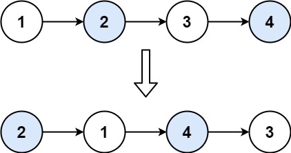
Example 2:
Input: head = []
Output: []
Example 3:
Input: head = [1]
Output: [1]
Example 4:
Input: head = [1,2,3]
Output: [2,1,3]
Constraints:
- The number of nodes in the list is in the range
[0, 100]. 0 <Node.val <= 100=
※ 2.7.13.1. Constraints and Edge Cases
<list constraints, input limits, or tricky edge cases here>
※ 2.7.13.2. My Solution (Code)
1: # Definition for singly-linked list. 2: # class ListNode: 3: # def __init__(self, val=0, next=None): 4: # self.val = val 5: # self.next = next 6: class Solution: 7: │ def swapPairs(self, head: Optional[ListNode]) -> Optional[ListNode]: 8: │ │ if (not head) or (head and not head.next): 9: │ │ │ return head 10: │ │ │ 11: │ │ dummy = ListNode() 12: │ │ prev = dummy 13: │ │ ptr = head 14: │ │ while (first:=ptr) and (second:=ptr.next): 15: │ │ │ next_join = second.next 16: │ │ │ second.next = first 17: │ │ │ first.next = next_join 18: │ │ │ prev.next = second 19: │ │ │ prev = first 20: │ │ │ ptr = next_join 21: │ │ │ 22: │ │ return dummy.next
here’s a recursive version of it:
1: class Solution: 2: │ def swapPairs(self, head: Optional[ListNode]) -> Optional[ListNode]: 3: │ │ if not head or not head.next: 4: │ │ │ return head 5: │ │ second = head.next 6: │ │ head.next = self.swapPairs(second.next) 7: │ │ second.next = head 8: │ │ return second
※ 2.7.13.3. My Approach/Explanation
Classic swapping logic
※ 2.7.13.4. My Learnings/Questions
- STYLE: walrus operator is really useful for this.
※ 2.7.13.5. [Optional] Additional Context
Morale Booster
※ 2.8. Trees
| Headline | Time | ||
|---|---|---|---|
| Total time | 7:36 | ||
| Trees | 7:36 | ||
| [45] Invert Binary Tree (226) | 0:44 | ||
| [46] Maximum Depth of Binary Tree (104) | 0:02 | ||
| [47] Diameter of Binary Tree (543) | 0:50 | ||
| [48] Balanced Binary Tree (110) | 0:50 | ||
| [49] Same Tree (100) | 0:23 | ||
| [50] Subtree of Another Tree (572) | 0:32 | ||
| [51] Lowest Common Ancestor of a… | 0:26 | ||
| [52] Binary Tree Level Order… | 0:10 | ||
| [53] Binary Tree Right Side View (199) | 0:29 | ||
| [54] Count Good Nodes in Binary Tree… | 0:27 | ||
| [55] Validate Binary Search Tree (98) | 0:25 | ||
| [56] Kth Smallest Element in BST (99) | 0:46 | ||
| [57] ⭐️ Construct Binary Tree from… | 0:08 | ||
| [58] Binary Tree Maximum Path Sum (124) | 0:33 | ||
| [59] Serialize and Deeserialize… | 0:51 |
※ 2.8.1. General Notes
※ 2.8.1.1. Notes
More verbose notes are found at the Notes section at the bottom of the document.
※ 2.8.1.1.1. Binary Trees are special
- it’s the building block of complex DS-es (Red Black, Multi-Way, Binary Heap, Graph, Tries, Union Find, Segment Tree)
- represents recursive thinking, and the common techniques can be seen as mapping the problems into tree-structures
techniques like:
- backtracking
- bfs
- DP
※ 2.8.1.1.2. Basics: Math
- full binary tree:
- number of nodes can be found using the geometric series = \(2^{h}-1\)
- as for height, it depends. On average it’s \(O(\log N)\) but at worst case, it can be \(O(N)\) if it’s skewed. (where \(N\) is the number of Nodes in the tree)
※ 2.8.1.1.3. Basics: Terminology
full binary tree not the same as complete binary tree:
full \(\implies\) all nodes in all levels are filled
complete \(\implies\) all levels, EXCEPT the last level, are fully filled

- Value Ordering: For every node in the tree, all nodes in its left subtree have values less than the value of the node, and all nodes in its right subtree have values greater than the value of the node. You can simply remember it as “left is smaller, right is bigger.”
- Because of the “left smaller, right bigger” property, we can quickly find a specific node or all nodes within a range in a BST. This is the advantage of BST.
※ 2.8.1.2. TODO Useful Algorithms [0/4]
※ 2.8.1.2.1. TODO Balanced Trees
※ 2.8.1.2.2. TODO order statistics
※ 2.8.1.2.3. TODO Interval Trees
※ 2.8.1.2.4. TODO Range Trees
※ 2.8.1.3. Tricks
- Property based tricks:
- Traversal Properties that we can exploit:
- Ability to reconstruct tree: You can reconstruct a tree from preorder + inorder, or postorder + inorder, but not from preorder + postorder alone (unless the tree is full).
- Partitioning Properties:
- Preorder Traversal
- The first element is always the root of the current subtree.
- Inorder Traversal
- The index of the root splits the array into left and right subtrees.
- Postorder Traversal
- Preorder Traversal
When they ask extension questions e.g. in the problem “Kth Smallest Element in a BST”, our first reach should try to augment trees into order-statistic trees.
Only after that should we consider things like auxiliary datastructures like a minHeap or whatsoever.
- Traversal Properties that we can exploit:
- I think when it comes to post-order DFS, I’m just going to rely on the recursive version. The iterative version is a little complex.
- More Pythonic Styles:
- Python supports chained comparison: so
lower < test < upperwill work- this operation is lazy
- this only evaluates the
testonce and breaks it down into(lower < test) and (test < upper). This means thattestcould have been an expensive expression to evaluate, but it will only be evaluated ONCE, and it also avoids redundant computation / unintended side-effects from multiple evaluations.
Using Python Generators as a way to avoid non-local states for easy value-generation.
Check out the “Construct Binary Tree from Preorder and Inorder Traversal”
- Python supports chained comparison: so
- Performance Improvements:
- Avoid building intermediate lists by directly building an existing list. A good example is in the “Binary Tree Level Order Traversal” problem
State threading is something that I should be able to articulate.
It’s more efficient to keep state as part of the function parameters or return values.
State threading is a technique where you pass state explicitly through function arguments, which can lead to better performance (stack allocation, cache locality), safer code (no globals), and easier reasoning (pure functions). It is especially intuitive and beneficial in recursive algorithms, dynamic programming, functional programming, and parsing.
Here’s a deeper dive into it:
Show/Hide Md Code│ **State threading** is a programming technique where you explicitly pass and update *state* through function calls or iterations, rather than relying on global variables or external state. This is not about OS-level threading or concurrency, but about *threading state* through your computation—making the state explicit, local, and often stack-allocated rather than heap-allocated or global. │ │ This approach is a powerful performance optimization and code clarity tool in several scenarios. │ │ ## **Why State Threading Improves Performance** │ │ - **Avoids global state:** Functions become pure and easier to reason about, which can enable compiler optimizations and safer parallelization. │ - **Reduces heap allocations:** By passing state explicitly, you can often keep temporary data on the stack, which is faster to allocate and free than the heap. │ - **Improves cache locality:** When state is kept local to the call stack or within tight loops, memory access patterns are more predictable and cache-friendly. │ │ ## **Examples Where State Threading Is Intuitive and Efficient** │ │ ### **1. Recursive Algorithms (e.g., DFS with Accumulated State)** │ │ Instead of using a global variable to accumulate results, you thread the accumulator through recursive calls: │ │ ```python │ def dfs(node, acc): │ │ if not node: │ │ │ return acc │ │ acc += node.val │ │ acc = dfs(node.left, acc) │ │ acc = dfs(node.right, acc) │ │ return acc │ ``` │ - **Benefit:** No global variables; the accumulator is always up-to-date and local to the call stack. │ │ ### **2. Dynamic Programming with Explicit State** │ │ In DP, especially with memoization, you often pass the current state (e.g., indices, remaining capacity) as function arguments rather than storing it globally: │ │ ```python │ def knapsack(i, remaining_weight, memo): │ │ if (i, remaining_weight) in memo: │ │ │ return memo[(i, remaining_weight)] │ │ # ...compute... │ │ memo[(i, remaining_weight)] = result │ │ return result │ ``` │ - **Benefit:** The state space is explicit, making the function reentrant and easier to debug. │ │ ### **3. Functional Programming (Immutability)** │ │ Functional languages like Haskell or Clojure rely heavily on state threading, as all state must be passed explicitly due to immutability. │ │ ```haskell │ sumTree :: Tree -> Int -> Int │ sumTree Empty acc = acc │ sumTree (Node v l r) acc = sumTree r (sumTree l (acc + v)) │ ``` │ - **Benefit:** No side effects, enabling aggressive compiler optimizations and easy parallelization. │ │ ### **4. In-Order Traversal with Threaded State (No Global Variables)** │ │ Suppose you want to collect the in-order traversal of a binary tree in a list: │ │ ```python │ def inorder(node, acc): │ │ if not node: │ │ │ return acc │ │ acc = inorder(node.left, acc) │ │ acc.append(node.val) │ │ acc = inorder(node.right, acc) │ │ return acc │ │ │ result = inorder(root, []) │ ``` │ - **Benefit:** No globals, no class variables, and the state (`acc`) is always current. │ │ ### **5. Parsing and Tokenization** │ │ In parsers, you often thread the current position (index or pointer) through recursive calls: │ │ ```python │ def parse_expr(tokens, pos): │ │ # parse something starting at pos │ │ # return new_pos, parsed_expr │ │ ... │ ``` │ - **Benefit:** No need for global or mutable parser state; the parser is easily reusable and testable. │ │ ## **Summary Table** │ │ | Use Case | How State Threading Helps | │ |-----------------------------------|--------------------------------------------------| │ | Recursive DFS/Tree Traversal | No globals, stack-local state, safer recursion | │ | Dynamic Programming | Clear state space, memoization, reentrancy | │ | Functional Programming | Enables pure functions, no side effects | │ | In-order/Pre-order Traversal | Cleaner code, no class or global state | │ | Parsing/Tokenization | Stateless, composable parsers | │ │ **In summary:** │ State threading is a technique where you pass state explicitly through function arguments, which can lead to better performance (stack allocation, cache locality), safer code (no globals), and easier reasoning (pure functions). It is especially intuitive and beneficial in recursive algorithms, dynamic programming, functional programming, and parsing. │ │ If you want a deep-dive into any specific example or a comparison with global state or class variables, let me know! │ │ [1] https://www.vaia.com/en-us/explanations/computer-science/computer-programming/threading-in-computer-science/ │ [2] https://www.geeksforgeeks.org/operating-systems/thread-states-in-operating-systems/ │ [3] https://www.techtarget.com/whatis/definition/thread │ [4] https://en.wikipedia.org/wiki/Thread_(computing) │ [5] https://www.studocu.com/in/document/vignan-institute-of-technology-and-science/computer-science/thread-states-types-multithreads/80754167 │ [6] https://www.cs.utexas.edu/~dahlin/Classes/UGOS/lectures/lec4.pdf │ [7] https://www.geeksforgeeks.org/operating-systems/thread-in-operating-system/ │ [8] https://www.sciencedirect.com/topics/computer-science/threaded-programming │ [9] https://www.reddit.com/r/computerscience/comments/1b1y7jv/what_are_the_importance_of_processes_and_threads/ │ [10] https://eng.libretexts.org/Courses/Delta_College/Introduction_to_Operating_Systems/09:_Threads/9.01:_Process_and_Threads
※ 2.8.1.4. Canonical Problems
※ 2.8.1.4.1. Island Problems
- usually possible with traversal solutions because it’s about reachability
※ 2.8.1.5. Key Sources of Error
※ 2.8.2. [45] Invert Binary Tree (226)
Given the root of a binary tree, invert the tree, and return its
root.
Example 1:
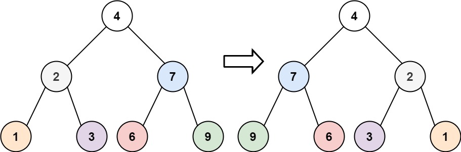
Input: root = [4,2,7,1,3,6,9] Output: [4,7,2,9,6,3,1]
Example 2:
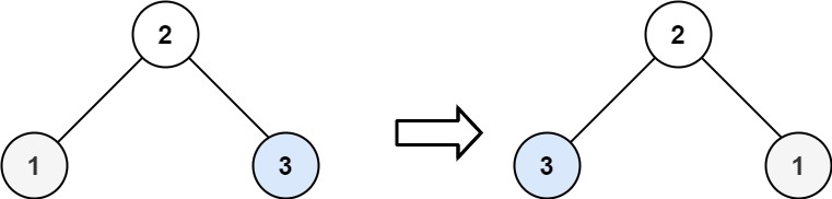
Input: root = [2,1,3] Output: [2,3,1]
Example 3:
Input: root = [] Output: []
Constraints:
- The number of nodes in the tree is in the range
[0, 100]. -100 <Node.val <= 100=
※ 2.8.2.1. Constraints and Edge Cases
- need to handle the empty case, just add an early return guard
※ 2.8.2.2. My Solution (Code)
※ 2.8.2.2.1. Iterative BFS
- Intuition:
- this is more like a top-down BFS because we are handling things level-by-level. We can do so because we’re not going to lose the pointers because of the working deque that we use to store the encountered nodes.
- Complexity Analysis:
- Time Complexity: \(O(N)\)
- Space Complexity: \(O(N)\) (queue can hold up to \(N/2\) nodes in worst case)
1: from collections import deque 2: 3: class Solution: 4: │ def invertTree(self, root: Optional[TreeNode]) -> Optional[TreeNode]: 5: │ │ if not root: 6: │ │ │ return root 7: │ │ queue = deque([root]) 8: │ │ while queue: 9: │ │ │ node = queue.popleft() 10: │ │ │ node.left, node.right = node.right, node.left 11: │ │ │ if node.left: 12: │ │ │ │ queue.append(node.left) 13: │ │ │ if node.right: 14: │ │ │ │ queue.append(node.right) 15: │ │ return root 16:
※ 2.8.2.2.2. Iterative DFS
- intuition:
- when adding into the stack for depth-first, that’s the point in time when we can do the inverting (swap left and right)
- the rest of the flow is just typical pre-order depth-first traversal iteratively
1: class Solution: 2: │ def invertTree(self, root: Optional[TreeNode]) -> Optional[TreeNode]: 3: │ │ if not root: 4: │ │ │ return root 5: │ │ stack = [root] 6: │ │ while stack: 7: │ │ │ node = stack.pop() 8: │ │ │ node.left, node.right = node.right, node.left 9: │ │ │ if node.left: 10: │ │ │ │ stack.append(node.left) 11: │ │ │ if node.right: 12: │ │ │ │ stack.append(node.right) 13: │ │ return root
※ 2.8.2.2.3. Recursive Post-Order DFS
- Complexity Analysis:
- Time
- since each node is visited only once, it’s \(O(N)\) time where \(N\) is the number of nodes
- Space
Space Complexity: Recursive stack: In the worst case (completely unbalanced tree), the recursion stack could grow to \(O(N)\).
Best case (balanced tree): Stack depth is \(O(\log N)\).
No additional data structures are used.
- Time
1: # Definition for a binary tree node. 2: # class TreeNode: 3: # def __init__(self, val=0, left=None, right=None): 4: # self.val = val 5: # self.left = left 6: # self.right = right 7: class Solution: 8: │ def invertTree(self, root: Optional[TreeNode]) -> Optional[TreeNode]: 9: │ │ if not root: 10: │ │ │ return root 11: │ │ right_inverted = self.invertTree(root.right) 12: │ │ left_inverted = self.invertTree(root.left) 13: │ │ 14: │ │ root.left, root.right = right_inverted, left_inverted 15: │ │ 16: │ │ return root
post order is because we need to flip it after we handle the children, so we entertain the root node last.
We can make it even cleaner by avoiding the extra variables (right_inverted and left_inverted)
1: 2: class Solution: 3: │ def invertTree(self, root: Optional[TreeNode]) -> Optional[TreeNode]: 4: │ │ if not root: 5: │ │ │ return root 6: │ │ │ 7: │ │ root.left, root.right = self.invertTree(root.right), self.invertTree(root.left) 8: │ │ 9: │ │ return root
※ 2.8.2.3. My Approach/Explanation
I find the recursive solution a lot more intuitive than the iterative. However, I feel like in general, to avoid space usage due to recursion stack frames, doing the iterative solution is the superior solution.
※ 2.8.2.4. My Learnings/Questions
- for complexity analysis, it seems that the intuition is as such:
- for space:
It DOESN’T MATTER IF RECURSIVE/ITERATIVE IMPLEMENTATION for the space USAGE. However, what space is used matters. Recursive solutions will use stack frames so there’s a higher chance of stack overflow.
Summary: The space complexity for binary tree traversals is O(h) (tree height) for both recursive and iterative implementations. However, recursive solutions use the call stack (risking stack overflow for deep trees), while iterative solutions use an explicit stack on the heap, which is typically less constrained.
is it a BFS?
If so, then the limiting factor in the tree for space is its breadth, so how fat the tree is \(\implies O(W)\) where \(W\) is the maximum number of nodes in any one level of the tree.
is it a DFS?
If so, then the limiting factor in the tree for space is its depth/height, so how deep the tree is: \(\implies O(H)\) where \(H\) is the height/depth of the tree.
- for time: All of them run at \(O(N)\) where \(N\) is the number of nodes in the tree because each node is processed once, regardless of the traversal approach.
- for space:
It DOESN’T MATTER IF RECURSIVE/ITERATIVE IMPLEMENTATION for the space USAGE. However, what space is used matters. Recursive solutions will use stack frames so there’s a higher chance of stack overflow.
Summary: The space complexity for binary tree traversals is O(h) (tree height) for both recursive and iterative implementations. However, recursive solutions use the call stack (risking stack overflow for deep trees), while iterative solutions use an explicit stack on the heap, which is typically less constrained.
- I think jumping into a BFS/DFS dichotomy might be a misstep because in the case of the “Invert Binary Tree” problem, note:
the iterative BFS works:
I initially thought of it as a DFS because the recursive solution was the most intuitive to me, however the iterative version made me realise that it could ALSO be seen as a BFS, in which we just have a working queue, and from the queue, we do the pointer re-assignments top-down, level-by-level.
the iterative DFS also works:
compared to the BFS variant (which uses a queue), the DFS variant uses a stack, which allows it to do depth-first traversals
Also the key intuition here is that we do the inversion as we are going through a pre-order iterative DFS traversal
QQ: how can I intuit the iterative approach? am i right in judging that the iterative approach is the more resource-friendly one? but is it more unreadable / hard to grasp?
AA: Intuition:
- The iterative approach mimics the recursive call stack with an explicit stack or queue. You process each node, swap its children, and add its children to the stack/queue.
- Resource-friendliness:
- Iterative: Avoids recursion stack, which can be important for very deep trees (prevents stack overflow).
- Recursive: More readable and concise, but uses the call stack.
- Readability: The recursive solution is generally more readable and intuitive for tree problems. The iterative version is more verbose but can be preferable in languages with small recursion stack limits.
※ 2.8.2.5. [Optional] Additional Context
It’s amazing that the recursive solution actually took me a minute to implement correctly.
※ 2.8.3. [46] Maximum Depth of Binary Tree (104)
Given the root of a binary tree, return its maximum depth.
A binary tree’s maximum depth is the number of nodes along the longest path from the root node down to the farthest leaf node.
Example 1:
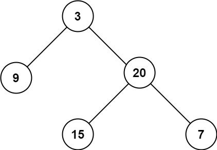
Input: root = [3,9,20,null,null,15,7] Output: 3
Example 2:
Input: root = [1,null,2] Output: 2
Constraints:
- The number of nodes in the tree is in the range
[0, 10=^{=4}=]=. -100 <Node.val <= 100=
※ 2.8.3.1. Constraints and Edge Cases
<list constraints, input limits, or tricky edge cases here>
※ 2.8.3.2. My Solution (Code)
※ 2.8.3.2.1. Recursive Post-Order DFS
1: class Solution: 2: │ def maxDepth(self, root: Optional[TreeNode]) -> int: 3: │ │ if not root: 4: │ │ │ return 0 5: │ │ │ 6: │ │ return max(self.maxDepth(root.left), self.maxDepth(root.right)) + 1 7:
※ 2.8.3.2.2. Iterative DFS
We’d need to use a stack to explore the depths.
Now for the case of tracking the depth, we can use a tuple for this and “annotate” it with the height.
When inserting the child nodes, that’s when we can add in their new heights.
Careful on the height values, they are 1-indexed.
1: class Solution: 2: │ def maxDepth(self, root: Optional[TreeNode]) -> int: 3: │ │ if not root: 4: │ │ │ return 0 5: │ │ │ 6: │ │ stack = [(root, 1)] 7: │ │ max_depth = 0 8: │ │ 9: │ │ while stack: 10: │ │ │ node, depth = stack.pop() 11: │ │ │ max_depth = max(max_depth, depth) 12: │ │ │ if node.left: 13: │ │ │ │ stack.append((node.left, depth + 1)) 14: │ │ │ if node.right: 15: │ │ │ │ stack.append((node.right, depth + 1)) 16: │ │ │ │ 17: │ │ return max_depth
※ 2.8.3.2.3. Iterative BFS
We can also go level-by-level and count the levels we see. Since we are going level by level, it’s a FIFO pattern that’s why we use a deque.
1: from collections import deque 2: 3: class Solution: 4: │ def maxDepth(self, root: Optional[TreeNode]) -> int: 5: │ │ if not root: 6: │ │ │ return 0 7: │ │ │ 8: │ │ queue = deque([root]) 9: │ │ depth = 0 10: │ │ 11: │ │ while queue: 12: │ │ │ # for all parents (each level), find their children: 13: │ │ │ for _ in range(len(queue)): 14: │ │ │ │ node = queue.popleft() 15: │ │ │ │ if node.left: 16: │ │ │ │ │ queue.append(node.left) 17: │ │ │ │ if node.right: 18: │ │ │ │ │ queue.append(node.right) 19: │ │ │ │ │ 20: │ │ │ depth += 1 21: │ │ │ 22: │ │ return depth
※ 2.8.3.3. My Approach/Explanation
Refer to the explanations above.
I prefer the level order traversal to calculate the level by level height.
※ 2.8.3.4. My Learnings/Questions
QQ still can’t get the intuition completely right for the iterative solution to this
AA Think of the stack as simulating the call stack of recursion. Each tuple (node, depth) represents a “work-in-progress” call to maxDepth. You push children with incremented depth as you would recurse, and the stack keeps track of which nodes you have to process next. Whenever you pop, you update the
max_depthif needed.for the iterative DFS, note how we can augment nodes by creating tuples with the statistics we need for them.
Exactly right! This is a powerful pattern for iterative tree/graph problems: you can “annotate” each node with any extra state you need (like depth, parent, path, etc.) by storing tuples or custom objects in your stack or queue.
※ 2.8.4. [47] Diameter of Binary Tree (543) redo post_order_dfs easy
Given the root of a binary tree, return the length of the diameter
of the tree.
The diameter of a binary tree is the length of the longest path
between any two nodes in a tree. This path may or may not pass through
the root.
The length of a path between two nodes is represented by the number of edges between them.
Example 1:
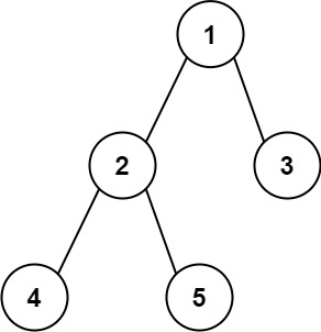
Input: root = [1,2,3,4,5] Output: 3 Explanation: 3 is the length of the path [4,2,1,3] or [5,2,1,3].
Example 2:
Input: root = [1,2] Output: 1
Constraints:
- The number of nodes in the tree is in the range
[1, 10=^{=4}=]=. -100 <Node.val <= 100=
※ 2.8.4.1. Constraints and Edge Cases
Nothing fancy
※ 2.8.4.2. My Solution (Code)
※ 2.8.4.2.1. Recursive Post-Order DFS
1: # Definition for a binary tree node. 2: # class TreeNode: 3: # def __init__(self, val=0, left=None, right=None): 4: # self.val = val 5: # self.left = left 6: # self.right = right 7: class Solution: 8: │ def diameterOfBinaryTree(self, root: Optional[TreeNode]) -> int: 9: │ │ max_diameter = 0 10: │ │ 11: │ │ # returns the max height for that node 12: │ │ def traverse(root: Optional[TreeNode]): 13: │ │ │ nonlocal max_diameter 14: │ │ │ if root is None: 15: │ │ │ │ return 0 16: │ │ │ # max height left 17: │ │ │ max_left = traverse(root.left) 18: │ │ │ # max height right 19: │ │ │ max_right = traverse(root.right) 20: │ │ │ # +2 because 2 extra edges as they connect with the current node 21: │ │ │ # QQ: why is it not +2 because of the 2 extra edges? 22: │ │ │ # combined = max_left + max_right + 2 23: │ │ │ combined = max_left + max_right 24: │ │ │ # compare with the global accumulator 25: │ │ │ max_diameter = max(max_diameter, combined) 26: │ │ │ 27: │ │ │ # returns the max height of either choices with an extra edge here 28: │ │ │ return max(max_left, max_right) + 1 29: │ │ │ 30: │ │ traverse(root) 31: │ │ 32: │ │ return max_diameter
I should have probably named it “length” instead of “height” since we’re getting the max length of the path there.
Your solution is correct. You use a post-order DFS to compute the height of each subtree. At each node, you calculate the sum of the left and right subtree heights (which is the number of edges in the longest path passing through that node). You update a global (nonlocal) maximum diameter accordingly. You return the maximum diameter at the end.
- Time and Space Complexity
- Time Complexity:
- Each node is visited once, so \(O(N)\) where \(N\) is the number of nodes.
- Space Complexity:
- Recursive stack: \(O(H)\), where \(H\) is the height of the tree (worst case \(O(N)\) for a skewed tree, \(O(log N)\) for a balanced tree).
- No extra data structures used.
- Time Complexity:
Here’s a cleaner version
1: class Solution: 2: │ def diameterOfBinaryTree(self, root: Optional[TreeNode]) -> int: 3: │ │ diameter = 0 4: │ │ 5: │ │ def height(node): 6: │ │ │ nonlocal diameter 7: │ │ │ if not node: 8: │ │ │ │ return 0 9: │ │ │ left = height(node.left) 10: │ │ │ right = height(node.right) 11: │ │ │ diameter = max(diameter, left + right) 12: │ │ │ return max(left, right) + 1 13: │ │ │ 14: │ │ height(root) 15: │ │ return diameter
※ 2.8.4.2.2. Post Order Iterative DFS:
- Intuition
- You need to know both children’s heights before you can compute the diameter at a node, so you must process the node after its children (post-order).
- The stack simulates the recursion, and the hashmap replaces the recursive return values for heights.
- Key Implementation Points:
heightsdictionary stores the computed height for each node after both children are processed.max_diameteris updated at each node using the sum of left and right subtree heights.- The traversal order is true post-order: left, right, root.
- This approach simulates the call stack and the return values of recursion explicitly, as described in
1: class Solution: 2: │ def diameterOfBinaryTree(self, root: Optional[TreeNode]) -> int: 3: │ │ if not root: 4: │ │ │ return 0 5: │ │ │ 6: │ │ stack = [] 7: │ │ heights = dict() # node -> height 8: │ │ max_diameter = 0 9: │ │ node = root 10: │ │ last_visited = None 11: │ │ 12: │ │ while stack or node: 13: │ │ │ # Go as left as possible 14: │ │ │ if node: 15: │ │ │ │ stack.append(node) 16: │ │ │ │ node = node.left 17: │ │ │ else: 18: │ │ │ │ peek = stack[-1] 19: │ │ │ │ # If right child exists and not yet processed 20: │ │ │ │ if peek.right and last_visited != peek.right: 21: │ │ │ │ │ node = peek.right 22: │ │ │ │ else: 23: │ │ │ │ │ # Both children processed, now process node itself 24: │ │ │ │ │ left_height = heights.get(peek.left, 0) 25: │ │ │ │ │ right_height = heights.get(peek.right, 0) 26: │ │ │ │ │ heights[peek] = 1 + max(left_height, right_height) 27: │ │ │ │ │ max_diameter = max(max_diameter, left_height + right_height) 28: │ │ │ │ │ last_visited = stack.pop() 29: │ │ │ │ │ node = None # Don't go down left again 30: │ │ │ │ │ 31: │ │ return max_diameter
※ 2.8.4.3. My Approach/Explanation
I want to be able to do a post order traversal by when I will have the max result of both left and right subtrees. For each subtree’s root, I need to do the following:
- try to join left and right up and see if that improves the accumulating score
- return the max height (best length)
※ 2.8.4.4. My Learnings/Questions
- Python:
- using
nonlocalvariable is faster than adding a custom attribute to the class, and it’s more pythonic as well. - here, we could have technically done a state-threading approach and that might have been a more performant way of implementing this.
- using
Left-bias iterative DFS and Right Bias Iterative DFS:
In this example, the recursive post order BFS is much simpler to reason with than the iterative version of the DFS. Post order DFS done iteratively is tricky.
In this case, just realise that the way to keep exploring the left-most branch is just by adding a while loop.
Show/Hide Python Code1: │ │ while stack or node: 2: │ │ │ # Go as left as possible 3: │ │ │ if node: 4: │ │ │ │ stack.append(node) 5: │ │ │ │ node = node.left 6: │ │ │ else:
For right-only DFS (preorder, right-first):
Push left child first, right child second (right on top, visited next)
This “mirrors” the standard stack order for left-branch-biased DFS.
Show/Hide Python Code1: stack = [root] 2: while stack: 3: │ node = stack.pop() 4: │ if node: 5: │ │ # process node 6: │ │ stack.append(node.left) 7: │ │ stack.append(node.right)
Why not +2? The height of a node is the number of edges from that node to its deepest leaf.
The diameter at a node is the sum of the left and right heights (number of edges from the deepest left leaf, up to the node, and down to the deepest right leaf).
No extra +2 is needed—you’re already counting edges, not nodes.
※ 2.8.5. [48] Balanced Binary Tree (110) state_threading
Given a binary tree, determine if it is height-balanced.
Example 1:
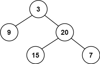
Input: root = [3,9,20,null,null,15,7] Output: true
Example 2:
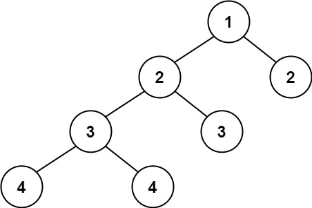
Input: root = [1,2,2,3,3,null,null,4,4] Output: false
Example 3:
Input: root = [] Output: true
Constraints:
- The number of nodes in the tree is in the range
[0, 5000]. -10=^{=4}= <= Node.val <= 10=4
※ 2.8.5.1. Constraints and Edge Cases
- remember that the definition for balanced includes a tolerance of a diff of 1, so it’s not an equality check it’s a diff-check that we need to do
※ 2.8.5.2. My Solution (Code)
For both the optimal solutions below,
Time Complexity:
- Both solutions are \(O(N)\), where \(N\) is the number of nodes, since each node is visited once.
Space Complexity:
- \(O(H)\), where \(H\) is the height of the tree, due to the recursion stack. In the worst case (skewed tree), this is \(O(N)\); in the best case (balanced tree), it is \(O(log N)\).
※ 2.8.5.2.1. Recursive Post-Order DFS
1: # Definition for a binary tree node. 2: # class TreeNode: 3: # def __init__(self, val=0, left=None, right=None): 4: # self.val = val 5: # self.left = left 6: # self.right = right 7: class Solution: 8: │ # checks if a binary tree is balanced 9: │ def isBalanced(self, root: Optional[TreeNode]) -> bool: 10: │ │ # trivially true: 11: │ │ if not root: 12: │ │ │ return True 13: │ │ │ 14: │ │ self.balanced = True 15: │ │ 16: │ │ def height(node: Optional[TreeNode]): 17: │ │ │ if not node: 18: │ │ │ │ return 0 19: │ │ │ left, right = height(node.left), height(node.right) 20: │ │ │ is_balanced = abs(left - right) <= 1 21: │ │ │ self.balanced = self.balanced and is_balanced 22: │ │ │ 23: │ │ │ return max(left, right) + 1 24: │ │ │ 25: │ │ height(root) 26: │ │ 27: │ │ return self.balanced
※ 2.8.5.2.2. Recursive Post-Order DFS with tuple returns (State Threading)
This just returns a tuple of (is_balanced, max_height), is supposedly much faster.
I really like this style.
Also remember to use tuples here instead of lists.
1: class Solution: 2: │ # checks if a binary tree is balanced 3: │ def isBalanced(self, root: Optional[TreeNode]) -> bool: 4: │ │ def height(root): 5: │ │ │ if not root: 6: │ │ │ │ return True, 0 7: │ │ │ left, right = height(root.left), height(root.right) 8: │ │ │ 9: │ │ │ # if subtrees are balanced and the height diff is tolerable 10: │ │ │ is_balanced = left[0] and right[0] and abs(left[1]-right[1]) <= 1 11: │ │ │ 12: │ │ │ return is_balanced, 1 + max(left[1], right[1]) 13: │ │ │ 14: │ │ return height(root)[0]
this version is even more idiomatic and has early returns to speed things up even more:
1: class Solution: 2: │ def isBalanced(self, root: Optional[TreeNode]) -> bool: 3: │ │ def check(node): 4: │ │ │ if not node: 5: │ │ │ │ return True, 0 6: │ │ │ left_balanced, left_height = check(node.left) 7: │ │ │ right_balanced, right_height = check(node.right) 8: │ │ │ 9: │ │ │ # introspect, then early returns: 10: │ │ │ if not left_balanced or not right_balanced: 11: │ │ │ │ return False, 0 12: │ │ │ # introspect, then early returns: 13: │ │ │ if abs(left_height - right_height) > 1: 14: │ │ │ │ return False, 0 15: │ │ │ │ 16: │ │ │ return True, 1 + max(left_height, right_height) 17: │ │ │ 18: │ │ return check(root)[0]
Here, as soon as an unbalanced subtree is found, the function returns immediately and does not continue to check further.
※ 2.8.5.3. My Approach/Explanation
Once again we have to do a post-order traversal, so recursive approach is my first-reach here.
I’m just going to return heights and then for each iteration, the post order operation that I do includes accumulating a boolean.
I suspect that I should be able to do some early returns from this, not sure what’s the best way to introduce that.
※ 2.8.5.4. My Learnings/Questions
- The post-order traversal is natural here because you need the heights of the children before you can determine if the current node is balanced.
- pythonic improvements:
- Use tuples instead of lists for fixed-size, immutable return values.
- Use descriptive variable names (
checkinstead ofheightfor the helper function). - Avoid using a class attribute (like
self.balanced) for local state in recursive functions.
- There’s an interesting speed up pattern avoids non local vars by just returning a tuple of
(is_balanced, height). It seems to be must faster. I quite like that trick. This is called a threaded state (where state is passed as function parameters or return values) – it makes the state explicit and local to each call-frame. - QQ: how do I optimise for time??
- remember that the definition for balanced includes a tolerance of a diff of 1, so it’s not an equality check it’s a diff-check that we need to do
Overloading class attr vs non local variable vs state threading
There’s a bunch of ways we can accumulate variables
Summary: Using a class attribute for recursion state is less safe and less clear than using a nonlocal variable or, ideally, threading state through arguments or return values. This keeps your recursive logic self-contained, avoids side effects, and makes your code easier to reason about and maintain
Here’s a comparison:
Show/Hide Md CodeThe suggestion to **avoid using a class attribute (like `self.balanced`) for local state in recursive functions** is rooted in best practices for code clarity, maintainability, and correctness. Here’s a comparison with using a `nonlocal` variable or other alternatives: ### **Why Avoid Class Attributes for Local Recursive State?** - **Scope Pollution:** │ Class attributes persist beyond the function call and are accessible anywhere in the class. This can lead to accidental modification or misuse elsewhere in your code, making bugs harder to track[5][6]. │ - **Thread Safety:** │ If your code ever runs in a multi-threaded context, class attributes can introduce race conditions and hard-to-find bugs, since they are shared across all method calls on an instance. │ - **Reentrancy:** │ If you call the same method recursively or from multiple places, the shared state can be overwritten, leading to incorrect results. │ - **Readability:** │ It’s less clear to readers that the attribute is only meant to be used within the context of a single recursive computation[5][6]. │ ### **Comparison: nonlocal vs. class attribute** | Method | Scope | Lifetime | Safety | Readability | Recommended? | |----------------------|------------------|------------------|------------------|--------------------|--------------| | **Class attribute** | Class/instance | Until object dies| Not thread-safe | Can be confusing | No | | **nonlocal variable**| Enclosing func | During function | Safer (local) | Clear intent | Yes | | **Threaded arg** | Function | Per call | Safest | Clearest | Yes (best) | - **nonlocal** is used for variables in an enclosing function scope (not global or class), so their lifetime is limited to the function call, making them safer and more predictable for recursion state[5][6]. - **Threading state through arguments** (i.e., passing state as function parameters or return values) is even better, as it makes the state explicit and local to each call frame[5][6]. ### **Best Practice** - **Use function arguments or return values to pass state** (most explicit, safest). - If you need to accumulate state in a helper function, use a `nonlocal` variable in an enclosing function. - **Avoid class attributes** for temporary, local state in recursive functions. ### **Example** #### Using a class attribute (not recommended): ```python class Solution: │ def isBalanced(self, root): │ │ self.balanced = True │ │ def check(node): │ │ │ # modifies self.balanced │ │ │ ... │ │ check(root) │ │ return self.balanced ``` #### Using nonlocal (better): ```python def isBalanced(self, root): │ balanced = True │ def check(node): │ │ nonlocal balanced │ │ ... │ check(root) │ return balanced ``` #### Passing state via return values (best): ```python def isBalanced(self, root): │ def check(node): │ │ # returns (is_balanced, height) │ │ ... │ return check(root)[0] ``` **Summary:** Using a class attribute for recursion state is less safe and less clear than using a `nonlocal` variable or, ideally, threading state through arguments or return values. This keeps your recursive logic self-contained, avoids side effects, and makes your code easier to reason about and maintain[5][6]. [1] https://understanding-recursion.readthedocs.io/en/latest/02%20Scope,%20Frame%20and%20Stack.html [2] https://realpython.com/python-recursion/ [3] https://www.reddit.com/r/Python/comments/4hkds8/do_you_recommend_using_recursion_in_python_why_or/ [4] https://stackoverflow.com/questions/1527354/recursive-function-best-practices-what-are-they [5] https://realpython.com/lessons/maintaining-state/ [6] https://realpython.com/python-thinking-recursively/ [7] https://www.interactivebrokers.com/campus/ibkr-quant-news/recursive-functions-in-python-concepts-types-and-applications-in-trading-part-i/ [8] https://developer.ibm.com/articles/l-recurs/ [9] https://realpython.com/inner-functions-what-are-they-good-for/ [10] https://www.youtube.com/watch?v=llnasP3Fnko
Also here’s some interesting info about state threading!
Show/Hide Md Code**State threading** is a programming technique where you explicitly pass and update *state* through function calls or iterations, rather than relying on global variables or external state. This is not about OS-level threading or concurrency, but about *threading state* through your computation—making the state explicit, local, and often stack-allocated rather than heap-allocated or global. This approach is a powerful performance optimization and code clarity tool in several scenarios. ## **Why State Threading Improves Performance** - **Avoids global state:** Functions become pure and easier to reason about, which can enable compiler optimizations and safer parallelization. - **Reduces heap allocations:** By passing state explicitly, you can often keep temporary data on the stack, which is faster to allocate and free than the heap. - **Improves cache locality:** When state is kept local to the call stack or within tight loops, memory access patterns are more predictable and cache-friendly. ## **Examples Where State Threading Is Intuitive and Efficient** ### **1. Recursive Algorithms (e.g., DFS with Accumulated State)** Instead of using a global variable to accumulate results, you thread the accumulator through recursive calls: ```python def dfs(node, acc): │ if not node: │ │ return acc │ acc += node.val │ acc = dfs(node.left, acc) │ acc = dfs(node.right, acc) │ return acc ``` - **Benefit:** No global variables; the accumulator is always up-to-date and local to the call stack. ### **2. Dynamic Programming with Explicit State** In DP, especially with memoization, you often pass the current state (e.g., indices, remaining capacity) as function arguments rather than storing it globally: ```python def knapsack(i, remaining_weight, memo): │ if (i, remaining_weight) in memo: │ │ return memo[(i, remaining_weight)] │ # ...compute... │ memo[(i, remaining_weight)] = result │ return result ``` - **Benefit:** The state space is explicit, making the function reentrant and easier to debug. ### **3. Functional Programming (Immutability)** Functional languages like Haskell or Clojure rely heavily on state threading, as all state must be passed explicitly due to immutability. ```haskell sumTree :: Tree -> Int -> Int sumTree Empty acc = acc sumTree (Node v l r) acc = sumTree r (sumTree l (acc + v)) ``` - **Benefit:** No side effects, enabling aggressive compiler optimizations and easy parallelization. ### **4. In-Order Traversal with Threaded State (No Global Variables)** Suppose you want to collect the in-order traversal of a binary tree in a list: ```python def inorder(node, acc): │ if not node: │ │ return acc │ acc = inorder(node.left, acc) │ acc.append(node.val) │ acc = inorder(node.right, acc) │ return acc │ result = inorder(root, []) ``` - **Benefit:** No globals, no class variables, and the state (`acc`) is always current. ### **5. Parsing and Tokenization** In parsers, you often thread the current position (index or pointer) through recursive calls: ```python def parse_expr(tokens, pos): │ # parse something starting at pos │ # return new_pos, parsed_expr │ ... ``` - **Benefit:** No need for global or mutable parser state; the parser is easily reusable and testable. ## **Summary Table** | Use Case | How State Threading Helps | |-----------------------------------|--------------------------------------------------| | Recursive DFS/Tree Traversal | No globals, stack-local state, safer recursion | | Dynamic Programming | Clear state space, memoization, reentrancy | | Functional Programming | Enables pure functions, no side effects | | In-order/Pre-order Traversal | Cleaner code, no class or global state | | Parsing/Tokenization | Stateless, composable parsers | **In summary:** State threading is a technique where you pass state explicitly through function arguments, which can lead to better performance (stack allocation, cache locality), safer code (no globals), and easier reasoning (pure functions). It is especially intuitive and beneficial in recursive algorithms, dynamic programming, functional programming, and parsing. If you want a deep-dive into any specific example or a comparison with global state or class variables, let me know! [1] https://www.vaia.com/en-us/explanations/computer-science/computer-programming/threading-in-computer-science/ [2] https://www.geeksforgeeks.org/operating-systems/thread-states-in-operating-systems/ [3] https://www.techtarget.com/whatis/definition/thread [4] https://en.wikipedia.org/wiki/Thread_(computing) [5] https://www.studocu.com/in/document/vignan-institute-of-technology-and-science/computer-science/thread-states-types-multithreads/80754167 [6] https://www.cs.utexas.edu/~dahlin/Classes/UGOS/lectures/lec4.pdf [7] https://www.geeksforgeeks.org/operating-systems/thread-in-operating-system/ [8] https://www.sciencedirect.com/topics/computer-science/threaded-programming [9] https://www.reddit.com/r/computerscience/comments/1b1y7jv/what_are_the_importance_of_processes_and_threads/ [10] https://eng.libretexts.org/Courses/Delta_College/Introduction_to_Operating_Systems/09:_Threads/9.01:_Process_and_Threads
※ 2.8.6. [49] Same Tree (100)
Given the roots of two binary trees p and q, write a function to
check if they are the same or not.
Two binary trees are considered the same if they are structurally identical, and the nodes have the same value.
Example 1:
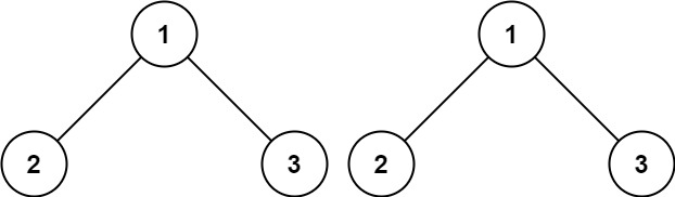
Input: p = [1,2,3], q = [1,2,3] Output: true
Example 2:
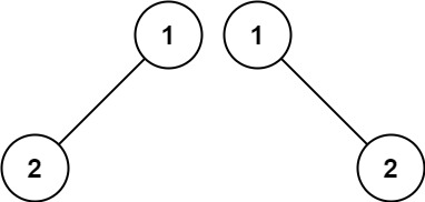
Input: p = [1,2], q = [1,null,2] Output: false
Example 3:
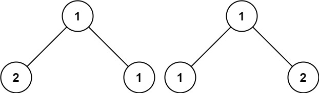
Input: p = [1,2,1], q = [1,1,2] Output: false
Constraints:
- The number of nodes in both trees is in the range
[0, 100]. -10=^{=4}= <= Node.val <= 10=4
※ 2.8.6.1. Constraints and Edge Cases
Nothing fancy
※ 2.8.6.2. My Solution (Code)
- Time Complexity:
- Both solutions are \(O(N)\), where \(N\) is the number of nodes (since each node is visited once).
- Space Complexity:
- Recursive: \(O(H)\), where \(H\) is the height of the tree (due to the call stack).
- Iterative: \(O(W)\), where \(W\) is the maximum width of the tree (due to the queue).
※ 2.8.6.2.1. Recursive Post-Order DFS
1: class Solution: 2: │ def isSameTree(self, p: Optional[TreeNode], q: Optional[TreeNode]) -> bool: 3: │ │ if bool(p) ^ bool(q): 4: │ │ │ return False 5: │ │ if not p and not q: 6: │ │ │ return True 7: │ │ if (p and not q) or (q and not p): 8: │ │ │ return False 9: │ │ │ 10: │ │ # QQ: this is evaluated lazily right? 11: │ │ is_same_subtrees = self.isSameTree(p.left, q.left) and self.isSameTree(p.right, q.right) 12: │ │ if not is_balanced_subtrees: 13: │ │ │ return False 14: │ │ │ 15: │ │ return p.val == q.val
Improvements:
- could have done a pre-order traversal instead, it’s more idomatic
There’s a more idiomatic pre-order traversal that we could have done instead of what we did above:
1: class Solution: 2: │ def isSameTree(self, p: Optional[TreeNode], q: Optional[TreeNode]) -> bool: 3: │ │ if not p and not q: 4: │ │ │ return True 5: │ │ if not p or not q: 6: │ │ │ return False 7: │ │ if p.val != q.val: 8: │ │ │ return False 9: │ │ │ 10: │ │ return self.isSameTree(p.left, q.left) and self.isSameTree(p.right, q.right) 11:
※ 2.8.6.2.2. Iterative BFS
The iterative process I used follows the same concept that they’ll all be similar. Also just uses tuples for supposedly equivalent nodes.
1: from collections import deque 2: class Solution: 3: │ def isSameTree(self, p: Optional[TreeNode], q: Optional[TreeNode]) -> bool: 4: │ │ queue = deque() 5: │ │ queue.append((p, q)) 6: │ │ while queue: 7: │ │ │ for _ in range(len(queue)): 8: │ │ │ │ node_p, node_q = queue.popleft() 9: │ │ │ │ 10: │ │ │ │ # allow for Nones 11: │ │ │ │ if not node_p and not node_q: 12: │ │ │ │ │ continue 13: │ │ │ │ │ 14: │ │ │ │ # check for mismatch: 15: │ │ │ │ if bool(node_p) ^ bool(node_q): 16: │ │ │ │ │ return False 17: │ │ │ │ │ 18: │ │ │ │ if node_p.val != node_q.val: 19: │ │ │ │ │ return False 20: │ │ │ │ │ 21: │ │ │ │ # accept it: 22: │ │ │ │ queue.append((node_p.left, node_q.left)) 23: │ │ │ │ queue.append((node_p.right, node_q.right)) 24: │ │ │ │ 25: │ │ return True
※ 2.8.6.2.3. Iterative DFS
1: class Solution: 2: │ def isSameTree(self, p: Optional[TreeNode], q: Optional[TreeNode]) -> bool: 3: │ │ stack = [(p, q)] 4: │ │ while stack: 5: │ │ │ node1, node2 = stack.pop() 6: │ │ │ if not node1 and not node2: 7: │ │ │ │ continue 8: │ │ │ if not node1 or not node2: 9: │ │ │ │ return False 10: │ │ │ if node1.val != node2.val: 11: │ │ │ │ return False 12: │ │ │ # Push children as pairs 13: │ │ │ stack.append((node1.right, node2.right)) 14: │ │ │ stack.append((node1.left, node2.left)) 15: │ │ return True
※ 2.8.6.3. My Approach/Explanation
I know that there’s some saying about a particular order of traversal that can be used to compare similarity / do serialisation & deserialisation but I don’t remember it.
AA: see this:
Unique Reconstruction │ │ - Given only inorder traversal, you can't reconstruct the tree: multiple trees can have the same inorder. │ │ - Given only preorder/postorder, you can't reconstruct the tree: same reason. │ │ - Given both inorder and preorder (or postorder), you can uniquely reconstruct the binary tree. │ │ │ │ - Preorder gives you the parents-first ordering, while inorder gives left/parent/right, which nails down the structure. │ │ Serialization (Practical Perspective): │ │ - In real world tree serialization (as in Leetcode), we typically do: │ │ │ │ - Preorder traversal (but must record "null"/None for missing children!), e.g.: │ │ - [root, left, left.left, None, left.right, None, None, right, ...] │ │ │ │ - This fully captures structure with a single traversal if you record nulls. │ │ │ - Classic textbook approach for reconstruction: │ │ │ │ - Inorder + Preorder │ │ │ │ - Inorder + Postorder │ │ Breadth-first (level order) with nulls also suffices.
So my solution I’ll go with is trying to simultaneously do 2 traversals in both the trees at the same time and then check that the logical values within each node is the same.
It’s a recursive post-order DFS that does a value-check.
※ 2.8.6.4. My Learnings/Questions
- Intuition: The core idea is to traverse both trees in the same order, always comparing corresponding nodes for both structure and value.
I like that the XOR works as intended, but I should prioritise readability.
The XOR (
bool(p) ^ bool(q)) works, but it’s less readable than if notpor notqafter you’ve already checked ifnot p and not q. The performance difference is negligible, but clarity is better with the standard idiom.Instead of the XOR, do this instead:
Show/Hide Python Code1: │ │ if not p and not q: 2: │ │ │ return True 3: │ │ if not p or not q: 4: │ │ │ return False 5: │ │ if p.val != q.val: 6: │ │ │ return False
- Completely Different Approaches
- DFS (iterative, with stack): You can use a stack instead of a queue, but the logic is the same as BFS.
- Tree Serialization:
Serialize both trees (e.g., pre-order with
Nonemarkers) and compare the resulting lists/strings. This is overkill for this problem but can be useful for tree equality in other contexts.
※ 2.8.6.5. [Optional] Additional Context
on the whole, I’ve been consistently doing well for these last few easy questions. I suppose this should be a morale boost + warm me up for the medium and hard questions that are expected to require some skill in mapping problems to the graph domain, which is probably where majority of the required effort will be.
Response: You’re right to feel good about your progress! These easy questions are foundational. Mastering them with clean, idiomatic code will make the transition to medium/hard problems much smoother. Keep practicing and building your intuition for traversals and recursion—you’re on the right track!
※ 2.8.7. [50] Subtree of Another Tree (572) sameness
Given the roots of two binary trees root and subRoot, return true
if there is a subtree of root with the same structure and node values
of= subRoot= and false otherwise.
A subtree of a binary tree tree is a tree that consists of a node in
tree and all of this node’s descendants. The tree tree could also be
considered as a subtree of itself.
Example 1:
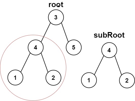
Input: root = [3,4,5,1,2], subRoot = [4,1,2] Output: true
Example 2:
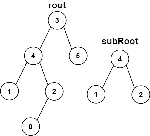
Input: root = [3,4,5,1,2,null,null,null,null,0], subRoot = [4,1,2] Output: false
Constraints:
- The number of nodes in the
roottree is in the range[1, 2000]. - The number of nodes in the
subRoottree is in the range[1, 1000]. -10=^{=4}= <= root.val <= 10=4-10=^{=4}= <= subRoot.val <= 10=4
※ 2.8.7.1. Constraints and Edge Cases
Nothing fancy.
※ 2.8.7.2. My Solution (Code)
- Time Complexity:
- Let \(n\) be the number of nodes in root and \(m\) in subRoot.
- In the worst case, for every node in root, you may need to compare an entire subtree of size up to \(m\).
- This leads to a worst-case time complexity of \(O(n * m)\).
- Let \(n\) be the number of nodes in root and \(m\) in subRoot.
- Space Complexity:
- The BFS queue can hold up to \(O(n)\) nodes in the worst case.
- The recursion stack for
is_samecan be up to \(O(m)\) deep, if the trees are skewed. - So, overall space complexity is \(O(max(n,m))\).
※ 2.8.7.2.1. Iterative BFS Traversal
1: from collections import deque 2: # Definition for a binary tree node. 3: # class TreeNode: 4: # def __init__(self, val=0, left=None, right=None): 5: # self.val = val 6: # self.left = left 7: # self.right = right 8: class Solution: 9: │ def isSubtree(self, root: Optional[TreeNode], subRoot: Optional[TreeNode]) -> bool: 10: │ │ if not root and not subRoot: 11: │ │ │ return True 12: │ │ │ 13: │ │ if not root or not subRoot: 14: │ │ │ return False 15: │ │ │ 16: │ │ def is_same(p: Optional[TreeNode], q: Optional[TreeNode]) -> bool: 17: │ │ │ if not p and not q: 18: │ │ │ │ return True 19: │ │ │ if not p or not q: 20: │ │ │ │ return False 21: │ │ │ if p.val != q.val: 22: │ │ │ │ return False 23: │ │ │ │ 24: │ │ │ return is_same(p.left, q.left) and is_same(p.right, q.right) 25: │ │ │ 26: │ │ queue = deque([root]) 27: │ │ while queue: 28: │ │ │ node = queue.popleft() 29: │ │ │ same = is_same(node, subRoot) 30: │ │ │ if same: 31: │ │ │ │ return True 32: │ │ │ else: 33: │ │ │ │ left, right = node.left, node.right 34: │ │ │ │ if left: 35: │ │ │ │ │ queue.append(left) 36: │ │ │ │ if right: 37: │ │ │ │ │ queue.append(right) 38: │ │ │ │ │ 39: │ │ return False
※ 2.8.7.2.2. Recursive BFS Traversal
1: class Solution: 2: │ def isSubtree(self, root: Optional[TreeNode], subRoot: Optional[TreeNode]) -> bool: 3: │ │ if not root: 4: │ │ │ return False 5: │ │ if self.is_same(root, subRoot): 6: │ │ │ return True 7: │ │ return self.isSubtree(root.left, subRoot) or self.isSubtree(root.right, subRoot) 8: │ │ 9: │ def is_same(self, p, q): 10: │ │ if not p and not q: 11: │ │ │ return True 12: │ │ if not p or not q: 13: │ │ │ return False 14: │ │ if p.val != q.val: 15: │ │ │ return False 16: │ │ return self.is_same(p.left, q.left) and self.is_same(p.right, q.right) 17:
※ 2.8.7.3. My Approach/Explanation
Intent here is that for subtree, it’s just similar to a subset concept. I can just do tree-sameness checks.
As long as one of the subtrees turns out to be equal, then I found a subtree.
As for the is_same checks, I can do it with early returns so that I avoid having to do too many duplicate operations on (potentially) valid portions of the subtree before rejection.
※ 2.8.7.4. My Learnings/Questions
- Intuition: The core idea is to check, at every node in root, whether the subtree rooted there is identical to subRoot. This is why a double traversal (outer for each node, inner for sameness) is required.
- python learnings:
The children enqueing can use an extends to do it in a single op: instead of
Show/Hide Python Codeif node.left: │ queue.append(node.left) if node.right: │ queue.append(node.right)
we can do
Show/Hide Python Codequeue.extend(child for child in (node.left, node.right) if child)
- This was a rare question that squarely got reduced to another question in a related area ( same tree problem ). That’s interesting.
Alternatives: there are two but they are a little more involved
The only way to improve time complexity for pathological cases (e.g., many repeated values) is to use advanced techniques like tree serialization with hashing or the Knuth-Morris-Pratt (KMP) algorithm, but those are rarely needed in practice for the given constraints.
Method 1: Serialise with hashing: How to Apply This Technique:
Step 1: Serialize both the main tree (root) and the subtree (subRoot) using a traversal, including markers for nulls.
Step 2: Compute a hash for each subtree in the main tree.
Step 3: Compute the hash for the subRoot serialization.
Step 4: Traverse the main tree, and for each node, compare the subtree hash with the subRoot hash. If they match, do a full comparison to confirm (to avoid hash collisions).
Show/Hide Python Code1: def serialize(node): 2: │ if not node: 3: │ │ return "#" 4: │ return f"{node.val},{serialize(node.left)},{serialize(node.right)}" 5: │ 6: def isSubtree(root, subRoot): 7: │ sub_serial = serialize(subRoot) 8: │ def dfs(node): 9: │ │ if not node: 10: │ │ │ return False 11: │ │ curr_serial = serialize(node) 12: │ │ if curr_serial == sub_serial: 13: │ │ │ return True 14: │ │ return dfs(node.left) or dfs(node.right) 15: │ return dfs(root) 16:
also instead of string comparison, we could do hash comparison by doing hash(serial)
- Advantages:
- Reduces repeated computation for identical subtrees.
- Subtree comparison becomes \(O(1)\) per node after serialization.
- Caveats:
- Hash collisions, while rare, are possible—so a final check is still needed.
- Serialization and hashing add extra space and pre-processing time.
- Advantages:
- Method 2: KMP Algorithm Read in the markdown brief below.
Read more about it here:
## Improving Subtree Matching with Advanced Techniques When the trees involved in the "Subtree of Another Tree" problem have many repeated values or repeated substructures, the naïve approach (checking every possible subtree with a full tree comparison) can become inefficient, leading to worst-case time complexity of $$O(n \cdot m)$$. Advanced techniques such as **tree serialization with hashing** and the **Knuth-Morris-Pratt (KMP) algorithm** can help optimize this process, especially for pathological cases. ### 1. Tree Serialization with Hashing #### **What is Tree Serialization?** Tree serialization is the process of converting a tree structure into a linear format (such as a string or list) that uniquely represents both the structure and the values of the tree. This is typically done using a traversal (pre-order, in-order, or post-order) with special markers for `null`/`None` children to avoid ambiguity. #### **How Does Hashing Help?** Hashing assigns a unique value (hash) to each subtree, so that subtree comparisons can be done in constant time by comparing hashes instead of the entire subtree structure and values. #### **How to Apply This Technique:** - **Step 1:** Serialize both the main tree (`root`) and the subtree (`subRoot`) using a traversal, including markers for nulls. - **Step 2:** Compute a hash for each subtree in the main tree. - **Step 3:** Compute the hash for the `subRoot` serialization. - **Step 4:** Traverse the main tree, and for each node, compare the subtree hash with the `subRoot` hash. If they match, do a full comparison to confirm (to avoid hash collisions). #### **Example:** ```python def serialize(node): │ if not node: │ │ return "#" │ return f"{node.val},{serialize(node.left)},{serialize(node.right)}" │ def isSubtree(root, subRoot): │ sub_serial = serialize(subRoot) │ def dfs(node): │ │ if not node: │ │ │ return False │ │ curr_serial = serialize(node) │ │ if curr_serial == sub_serial: │ │ │ return True │ │ return dfs(node.left) or dfs(node.right) │ return dfs(root) ``` - To improve further, you can use a hash function (e.g., `hash(serial)`) instead of direct string comparison for efficiency. #### **Advantages:** - Reduces repeated computation for identical subtrees. - Subtree comparison becomes $$O(1)$$ per node after serialization. #### **Caveats:** - Hash collisions, while rare, are possible—so a final check is still needed. - Serialization and hashing add extra space and preprocessing time. ### 2. Knuth-Morris-Pratt (KMP) Algorithm for Subtree Matching #### **What is KMP?** KMP is a classic string matching algorithm that finds all occurrences of a "pattern" string within a "text" string in linear time, $$O(N + M)$$, by preprocessing the pattern to avoid redundant comparisons. #### **How is KMP Applied to Trees?** - **Step 1:** Serialize both the main tree and the subtree (as above), using a traversal with null markers to uniquely capture structure. - **Step 2:** Treat the serialized main tree as the "text" and the serialized subtree as the "pattern." - **Step 3:** Use KMP to search for the pattern within the text. #### **Example:** ```python def serialize(node): │ if not node: │ │ return "#" │ return f",{node.val}{serialize(node.left)}{serialize(node.right)}" │ def kmp_search(text, pattern): │ # Build the partial match table (lps array) │ lps = [0] * len(pattern) │ j = 0 │ for i in range(1, len(pattern)): │ │ while j > 0 and pattern[i] != pattern[j]: │ │ │ j = lps[j-1] │ │ if pattern[i] == pattern[j]: │ │ │ j += 1 │ │ │ lps[i] = j │ # Search │ j = 0 │ for i in range(len(text)): │ │ while j > 0 and text[i] != pattern[j]: │ │ │ j = lps[j-1] │ │ if text[i] == pattern[j]: │ │ │ j += 1 │ │ if j == len(pattern): │ │ │ return True │ return False │ def isSubtree(root, subRoot): │ s = serialize(root) │ t = serialize(subRoot) │ return kmp_search(s, t) ``` #### **Advantages:** - Efficiently finds all matches of the subtree serialization in the main tree serialization. - Handles repeated values and structures gracefully, avoiding redundant work. #### **Caveats:** - Requires careful serialization to avoid false positives (e.g., two different trees with the same values in different structures). - Slightly more complex to implement than direct comparison. ### 3. When Are These Techniques Useful? - When the main tree is very large and contains many repeated values or substructures, making the naïve $$O(n \cdot m)$$ approach slow. - When you need to perform multiple subtree queries efficiently. - When you want to leverage string-matching optimizations for tree problems. ### 4. Summary Table | Technique | Core Idea | Time Complexity | Space Complexity | Use Case | |-----------------------------|--------------------------|-----------------|------------------|-----------------------------------------| | Naïve double traversal | Compare at every node | $$O(n \cdot m)$$| $$O(h)$$ | Simple, small trees | | Serialization + Hashing | Compare hashes | $$O(n + m)$$ | $$O(n + m)$$ | Large trees, repeated subtrees | | Serialization + KMP | String pattern matching | $$O(n + m)$$ | $$O(n + m)$$ | Large trees, repeated values/structures | **In practice, for LeetCode constraints, the naïve approach is usually sufficient, but understanding these advanced techniques is valuable for handling larger-scale or more complex tree matching problems.**
※ 2.8.7.5. [Optional] Additional Context
Finally got the iterative solution out first!
※ 2.8.8. [51] Lowest Common Ancestor of a Binary Search Tree (235) BST
Given a binary search tree (BST), find the lowest common ancestor (LCA) node of two given nodes in the BST.
According to the
definition of
LCA on Wikipedia: “The lowest common ancestor is defined between two
nodes p and q as the lowest node in T that has both p and q as
descendants (where we allow a node to be a descendant of itself).”
Example 1:
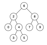
Input: root = [6,2,8,0,4,7,9,null,null,3,5], p = 2, q = 8 Output: 6 Explanation: The LCA of nodes 2 and 8 is 6.
Example 2:
Input: root = [6,2,8,0,4,7,9,null,null,3,5], p = 2, q = 4 Output: 2 Explanation: The LCA of nodes 2 and 4 is 2, since a node can be a descendant of itself according to the LCA definition.
Example 3:
Input: root = [2,1], p = 2, q = 1 Output: 2
Constraints:
- The number of nodes in the tree is in the range
[2, 10=^{=5}=]=. -10=^{=9}= <= Node.val <= 10=9- All
Node.valare unique. p !q=pandqwill exist in the BST.
※ 2.8.8.1. Constraints and Edge Cases
- target nodes will for sure be in the tree
- tree won’t be empty
- no duplicate values
※ 2.8.8.2. My Solution (Code)
※ 2.8.8.2.1. Optimal Solution (BST Order-based traversal)
this exploits the order property of BSTs
This can be written iteratively
1: class Solution: 2: │ def lowestCommonAncestor(self, root: 'TreeNode', p: 'TreeNode', q: 'TreeNode') -> 'TreeNode': 3: │ │ curr = root 4: │ │ while curr: 5: │ │ │ if p.val < curr.val and q.val < curr.val: 6: │ │ │ │ curr = curr.left 7: │ │ │ elif p.val > curr.val and q.val > curr.val: 8: │ │ │ │ curr = curr.right 9: │ │ │ else: 10: │ │ │ │ return curr
Or can be written recursively also:
1: class Solution: 2: │ def lowestCommonAncestor(self, root: 'TreeNode', p: 'TreeNode', q: 'TreeNode') -> 'TreeNode': 3: │ │ if p.val < root.val and q.val < root.val: 4: │ │ │ return self.lowestCommonAncestor(root.left, p, q) 5: │ │ if p.val > root.val and q.val > root.val: 6: │ │ │ return self.lowestCommonAncestor(root.right, p, q) 7: │ │ return root
- Optimal Solution’s Intuition:
- If both p and q are less than the current node, LCA is in the left subtree.
- If both are greater, LCA is in the right subtree.
- Otherwise, the current node is the LCA.
- Complexity Analysis
- Time Complexity: \(O(H)\) (height of tree)
- Space Complexity: \(O(1)\) (no extra structures)
※ 2.8.8.2.2. Initial Attempt
Silly mistakes here, correct intent though
Mistakes:
- the assignment
found_q = Trueis accidentally an equality check because of the== - parent tracing loop has issues:
- the
p_ptris not being advanced so this gives an infinite loop
- the
- Incorrect tracing in
q’s parent tracing and return- should check if the current node is in
p_parents, before moving to its parent q_ptris never updated \(\implies\) infinite loop
- should check if the current node is in
1: class Solution: 2: │ def lowestCommonAncestor(self, root: 'TreeNode', p: 'TreeNode', q: 'TreeNode') -> 'TreeNode': 3: │ │ stack = [root] 4: │ │ 5: │ │ # parent map 6: │ │ node_to_parent = {} 7: │ │ found_p, found_q = False, False 8: │ │ 9: │ │ while stack: 10: │ │ │ node = stack.pop() 11: │ │ │ if node == p: 12: │ │ │ │ found_p = True 13: │ │ │ if node == q: 14: │ │ │ │ found_q == True 15: │ │ │ │ 16: │ │ │ # early return from the DFS 17: │ │ │ if found_p and found_q: 18: │ │ │ │ break 19: │ │ │ │ 20: │ │ │ if node.left: 21: │ │ │ │ node_to_parent[node.left] = node 22: │ │ │ │ stack.append(node.left) 23: │ │ │ │ 24: │ │ │ if node.right: 25: │ │ │ │ node_to_parent[node.right] = node 26: │ │ │ │ stack.append(node.right) 27: │ │ │ │ 28: │ │ p_parents, q_parents = set(), set() 29: │ │ p_ptr, q_ptr = p, q 30: │ │ while p_ptr != root: 31: │ │ │ p_parents.add(node_to_parent[p_ptr]) 32: │ │ │ 33: │ │ while q_ptr != root: 34: │ │ │ parent = node_to_parent[q_ptr] 35: │ │ │ if q_ptr in p_parents: 36: │ │ │ │ return q_ptr 37: │ │ │ else: 38: │ │ │ │ q_parents.add(parent) 39: │ │ │ │ 40: │ │ return root 41:
- Time Complexity:
- Building the parent map: \(O(N)\) (each node visited once).
- Tracing ancestors: \(O(H)\) for each of \(p\) and \(q\) (\(H\) = height of tree).
- Total: \(O(N)\).
- Space Complexity:
- Parent map: \(O(N)\).
- Ancestor sets: \(O(H)\).
- Total: \(O(N)\).
1: class Solution: 2: │ def lowestCommonAncestor(self, root: 'TreeNode', p: 'TreeNode', q: 'TreeNode') -> 'TreeNode': 3: │ │ stack = [root] 4: │ │ 5: │ │ # parent map 6: │ │ node_to_parent = {} 7: │ │ found_p, found_q = False, False 8: │ │ 9: │ │ while stack: 10: │ │ │ node = stack.pop() 11: │ │ │ if node == p: 12: │ │ │ │ found_p = True 13: │ │ │ if node == q: 14: │ │ │ │ found_q = True 15: │ │ │ │ 16: │ │ │ # early return from the DFS 17: │ │ │ if found_p and found_q: 18: │ │ │ │ break 19: │ │ │ │ 20: │ │ │ if node.left: 21: │ │ │ │ node_to_parent[node.left] = node 22: │ │ │ │ stack.append(node.left) 23: │ │ │ │ 24: │ │ │ if node.right: 25: │ │ │ │ node_to_parent[node.right] = node 26: │ │ │ │ stack.append(node.right) 27: │ │ │ │ 28: │ │ # updated this to include p and q within the set. 29: │ │ p_parents, q_parents = {p}, {q} 30: │ │ p_ptr, q_ptr = p, q 31: │ │ while p_ptr != root: 32: │ │ │ parent = node_to_parent[p_ptr] 33: │ │ │ p_parents.add(parent) 34: │ │ │ p_ptr = parent 35: │ │ │ 36: │ │ # updated this to be simpler + considers q 37: │ │ while q_ptr != root: 38: │ │ │ if q_ptr in p_parents: 39: │ │ │ │ return q_ptr 40: │ │ │ q_ptr = node_to_parent[q_ptr] 41: │ │ │ 42: │ │ return root
※ 2.8.8.3. My Approach/Explanation
I have to keep track of parents somehow. An adjacency list came to mind, I guess in this case it’s more of a parent ref map (hashmap) that works.
This allows me to build up the parents until I dfs search the two (p and q). Once they’re found, I can return early!
Then I take the parent-map and I need to do membership checks so I use two sets to compare them. I build up a reference (p_parents) and allow the navigation up q’s parents to do membership checks.
The base case is to just return root since it’s guaranteed both p and q will be in the tree for sure.
※ 2.8.8.4. My Learnings/Questions
My initial approach did not exploit the BST’s ordering properties.
The LCA is the first node you encounter, traversing from root, where p and q split into different subtrees (or one is the current node).
This meant that I have unnecessary parent mapping.
However, this approach would work well for general trees (non-BSTs)
- Optimal Solution’s Intuition:
- If both p and q are less than the current node, LCA is in the left subtree.
- If both are greater, LCA is in the right subtree.
- Otherwise, the current node is the LCA.
- Optimal Solution’s Intuition:
- For interviews: Always clarify if the tree is a BST—if so, use the optimized approach.
※ 2.8.8.5. [Optional] Additional Context
Have to be a lot more careful, the silly mistakes are a sad thing since the approach is correct here.
※ 2.8.9. [52] Binary Tree Level Order Traversal (102)
Given the root of a binary tree, return the level order traversal of
its nodes’ values. (i.e., from left to right, level by level).
Example 1:
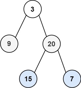
Input: root = [3,9,20,null,null,15,7] Output: [[3],[9,20],[15,7]]
Example 2:
Input: root = [1] Output: [[1]]
Example 3:
Input: root = [] Output: []
Constraints:
- The number of nodes in the tree is in the range
[0, 2000]. -1000 <Node.val <= 1000=
※ 2.8.9.1. Constraints and Edge Cases
<list constraints, input limits, or tricky edge cases here>
※ 2.8.9.2. My Solution (Code)
- complexity analysis:
- Time Complexity: \(O(N)\), where \(N\) is the number of nodes. Every node is visited once
- Space Complexity: \(O(N)\), for the queue and the output list. In the worst case (a complete tree), the queue may hold up to half the nodes at the last leve
※ 2.8.9.2.1. Initial Solution
1: from collections import deque 2: # Definition for a binary tree node. 3: # class TreeNode: 4: # def __init__(self, val=0, left=None, right=None): 5: # self.val = val 6: # self.left = left 7: # self.right = right 8: class Solution: 9: │ def levelOrder(self, root: Optional[TreeNode]) -> List[List[int]]: 10: │ │ if not root: 11: │ │ │ return [] 12: │ │ │ 13: │ │ queue = deque([root]) 14: │ │ layers = [] 15: │ │ 16: │ │ while queue: 17: │ │ │ layer = [] 18: │ │ │ for _ in range(len(queue)): 19: │ │ │ │ node = queue.popleft() 20: │ │ │ │ layer.append(node.val) 21: │ │ │ │ if node.left: 22: │ │ │ │ │ queue.append(node.left) 23: │ │ │ │ if node.right: 24: │ │ │ │ │ queue.append(node.right) 25: │ │ │ │ │ 26: │ │ │ layers.append(layer) 27: │ │ │ 28: │ │ return layers 29:
※ 2.8.9.2.2. Faster solution:
This is inspired by the other submissions for the question
1: class Solution: 2: │ def levelOrder(self, root: Optional[TreeNode]) -> List[List[int]]: 3: │ │ if not root: 4: │ │ │ return [] 5: │ │ levels = [] 6: │ │ queue = deque([(root, 0)]) # Start at level 0 7: │ │ 8: │ │ while queue: 9: │ │ │ node, level = queue.popleft() 10: │ │ │ if len(levels) == level: 11: │ │ │ │ levels.append([]) 12: │ │ │ levels[level].append(node.val) 13: │ │ │ if node.left: 14: │ │ │ │ queue.append((node.left, level + 1)) 15: │ │ │ if node.right: 16: │ │ │ │ queue.append((node.right, level + 1)) 17: │ │ return levels
※ 2.8.9.2.3. Recursive level order traversal with state threading (Pre-order DFS)
Here’s an alternative:
1: class Solution: 2: │ def levelOrder(self, root: Optional[TreeNode]) -> List[List[int]]: 3: │ │ levels = [] 4: │ │ def dfs(node, level): 5: │ │ │ if not node: 6: │ │ │ │ return 7: │ │ │ if len(levels) == level: 8: │ │ │ │ levels.append([]) 9: │ │ │ levels[level].append(node.val) 10: │ │ │ dfs(node.left, level + 1) 11: │ │ │ dfs(node.right, level + 1) 12: │ │ if root: 13: │ │ │ dfs(root, 0) 14: │ │ return levels
※ 2.8.9.3. My Approach/Explanation
- standard stuff
- seems like the population is faster when they avoid the extra
layerslist and straight away maintain acurr_leveland straightaway add to the final list
※ 2.8.9.4. My Learnings/Questions
Check out the augmented stack with the level value within it. This allows to consistently modify only the main
levelslist instead of building intermediate lists.Also it’s cool that the implementation for that is a pre-order DFS, even though the first-reach thought is that we should do a BFS.
※ 2.8.10. [53] Binary Tree Right Side View (199) right_first_traversal
Given the root of a binary tree, imagine yourself standing on the
right side of it, return the values of the nodes you can see ordered
from top to bottom.
Example 1:
Input: root = [1,2,3,null,5,null,4]
Output: [1,3,4]
Explanation:
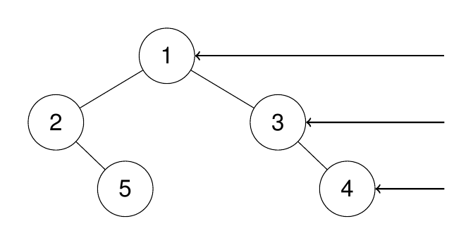
Example 2:
Input: root = [1,2,3,4,null,null,null,5]
Output: [1,3,4,5]
Explanation:

Example 3:
Input: root = [1,null,3]
Output: [1,3]
Example 4:
Input: root = []
Output: []
Constraints:
- The number of nodes in the tree is in the range
[0, 100]. -100 <Node.val <= 100=
※ 2.8.10.1. Constraints and Edge Cases
- Nothing much
※ 2.8.10.2. My Solution (Code)
※ 2.8.10.2.1. BFS, take last
1: from collections import deque 2: # Definition for a binary tree node. 3: # class TreeNode: 4: # def __init__(self, val=0, left=None, right=None): 5: # self.val = val 6: # self.left = left 7: # self.right = right 8: class Solution: 9: │ def rightSideView(self, root: Optional[TreeNode]) -> List[int]: 10: │ │ if not root: 11: │ │ │ return [] 12: │ │ │ 13: │ │ queue = deque([root]) 14: │ │ res = [] 15: │ │ while queue: 16: │ │ │ last = queue[-1] 17: │ │ │ res.append(last.val) 18: │ │ │ for _ in range(len(queue)): 19: │ │ │ │ node = queue.popleft() 20: │ │ │ │ 21: │ │ │ │ if node.left: 22: │ │ │ │ │ queue.append(node.left) 23: │ │ │ │ │ 24: │ │ │ │ if node.right: 25: │ │ │ │ │ queue.append(node.right) 26: │ │ │ │ │ 27: │ │ return res
※ 2.8.10.2.2. Right-biased DFS solution (initially fumbled)
The optimal DFS approach is to do a right-first traversal and record the first node encountered at each depth. This is iterative DFS (right first , stack based)
Key: Push left before right so the right child is processed first (stack is LIFO) –> this is a great example of right-bias DFS
1: class Solution: 2: │ def rightSideView(self, root: Optional[TreeNode]) -> List[int]: 3: │ │ if not root: 4: │ │ │ return [] 5: │ │ res = [] 6: │ │ stack = [(root, 0)] # (node, depth) 7: │ │ while stack: 8: │ │ │ node, depth = stack.pop() 9: │ │ │ if node: 10: │ │ │ │ if depth == len(res): 11: │ │ │ │ │ res.append(node.val) 12: │ │ │ │ # Push left first so right is processed first 13: │ │ │ │ stack.append((node.left, depth + 1)) 14: │ │ │ │ stack.append((node.right, depth + 1)) 15: │ │ return res 16:
And here’s the recursive version:
1: class Solution: 2: │ def rightSideView(self, root: Optional[TreeNode]) -> List[int]: 3: │ │ res = [] 4: │ │ def dfs(node, depth): 5: │ │ │ if not node: 6: │ │ │ │ return 7: │ │ │ if depth == len(res): 8: │ │ │ │ res.append(node.val) 9: │ │ │ dfs(node.right, depth + 1) 10: │ │ │ dfs(node.left, depth + 1) 11: │ │ dfs(root, 0) 12: │ │ return res 13:
Key: Visit right child before left, and record the first node at each depth
I fumbled this DFS approach because I was hasty
1: class Solution: 2: │ def rightSideView(self, root: Optional[TreeNode]) -> List[int]: 3: │ │ if not root: 4: │ │ │ return [] 5: │ │ │ 6: │ │ res = [] 7: │ │ stack = [root] 8: │ │ prev_parent = None 9: │ │ 10: │ │ while stack: 11: │ │ │ node = stack.pop() 12: │ │ │ res.append(node.val) 13: │ │ │ 14: │ │ │ if node.right: 15: │ │ │ │ stack.append(node.right) 16: │ │ │ │ continue 17: │ │ │ │ 18: │ │ │ if node.left: 19: │ │ │ │ stack.append(node.left) 20: │ │ │ │ continue 21: │ │ │ │ 22: │ │ │ if prev_parent and prev_parent.left: 23: │ │ │ │ node = prev_parent.left 24: │ │ │ │ if node.right: 25: │ │ │ │ │ stack.append(node.right) 26: │ │ │ │ │ continue 27: │ │ │ │ if node.left: 28: │ │ │ │ │ stack.append(node.left) 29: │ │ │ │ │ 30: │ │ │ prev_parent = node 31: │ │ │ 32: │ │ │ 33: │ │ return res 34:
❌ What’s Wrong in Your Code (Briefly):
No level tracking
You’re using a stack (DFS) without tracking the depth/level of each node.
As a result, you’re appending every visited node’s value to res, not just the rightmost one per level.
Incorrect traversal logic
You try to prioritize right children (which is good), but the logic with prevparent and continue statements is convoluted and doesn’t ensure you’re capturing the first node seen at each level.
Appending too many nodes
res.append(node.val) happens for every node, not just the first one seen at a new level from the right side.
No depth-based filtering
The correct solution should only append a node to res if it’s the first node encountered at that depth.
※ 2.8.10.3. My Approach/Explanation
- If I go level by level, and for each level, I just take whatever is on the rightmost in that left, then I get the right-sided view.
※ 2.8.10.4. My Learnings/Questions
- the BFS solution is so clean,
for the DFS, there’s a new insight here. If we wanna prioritise exploring the right branches each time, we just need to push the left ones on stack and carry on.
this automatically handles the backtracking because when there’s nothing else to do for the current stack, the left side can still resume and we keep walking down until the levels don’t overlap and now we can add new values to our result.
Here’s a more elaborate description of this point
Show/Hide Python Code1: Your learning is **correct and well-aligned with standard DFS right-side view strategies**. Here’s the verification and some extra context: 2: 3: > **Learning:** 4: > For DFS, if we want to prioritize exploring the right branches each time, we just need to push the left ones on the stack and carry on. 5: > This automatically handles the backtracking because when there's nothing else to do for the current stack, the left side can still resume and we keep walking down until the levels don't overlap and now we can add new values to our result. 6: 7: ### **Verification and Explanation** 8: 9: - **Right-First Traversal:** 10: │ The key insight is that in DFS, if you always visit the right child before the left child (i.e., for a stack, push left first so right is processed first), you ensure that at each depth, the first node you encounter is the rightmost node at that level[1][2][7]. 11: │ 12: - **Backtracking is Handled by the Stack:** 13: │ The stack naturally manages backtracking. When you finish exploring the right subtree, the left subtree is still on the stack and will be processed next. If you track the current depth and only add a node to your result when you first reach a new depth, you guarantee that only the rightmost node at each level is recorded[1][2][7]. 14: │ 15: - **Why This Works:** 16: │ - At each level, the first node you visit (thanks to right-first traversal) is the rightmost node visible from that side. 17: │ - By only adding to the result when you first reach a new depth, you avoid including left-side nodes when a right-side node exists at the same level. 18: │ 19: - **Implementation Pattern:** 20: │ - For iterative DFS, push `(node.left, depth+1)` before `(node.right, depth+1)` onto the stack so the right child is processed first. 21: │ - For recursive DFS, call `dfs(node.right, depth+1)` before `dfs(node.left, depth+1)`[1][2][7]. 22: │ 23: ### **References from Search Results** 24: 25: - [Vultr Docs][1]: “Perform a DFS traversal where you visit a node’s right child before its left child… If you reach a node at a depth you haven’t seen before (i.e., the depth is greater than the current size of the result list), that node is the first one encountered at that depth – which, because of the right-first order, is the rightmost node at that level.” 26: - [DesignGurus][2]: “To get the right side view using DFS, we should ensure we visit the right side of each level first… If you reach a node at a depth you haven’t seen before, that node is the rightmost node at that level.” 27: - [FinalRoundAI][7]: “Visit right subtree first, then left… If this is the first time we're seeing this level, this node is the rightmost for this level.” 28: 29: **In summary:** 30: Your understanding is correct. Prioritizing right children in DFS (by stack or recursion order) ensures the rightmost nodes are handled first, and the stack/recursion naturally manages the backtracking to left children. Tracking depth and only adding the first node at each depth gives you the right side view efficiently. 31: 32: Let me know if you want a visual walkthrough or more code examples! 33: 34: [1] https://docs.vultr.com/problem-set/binary-tree-right-side-view 35: [2] https://www.designgurus.io/answers/detail/199-binary-tree-right-side-view-vr36 36: [3] https://algo.monster/liteproblems/199 37: [4] https://leetcode.com/problems/binary-tree-right-side-view/ 38: [5] https://www.youtube.com/watch?v=WYCrIQ6Eekg 39: [6] https://blog.heycoach.in/right-side-view-of-a-binary-tree/ 40: [7] https://www.finalroundai.com/articles/tree-right-view-algorithm 41: [8] https://www.geeksforgeeks.org/dsa/print-right-view-binary-tree-2/ 42: [9] https://medium.programmerscareer.com/leetcode-199-golang-binary-tree-right-side-view-medium-depth-first-search-dfs-3aa7ad00670b 43: [10] https://www.educative.io/courses/decode-the-coding-interview-go/binary-tree-right-side-view
- as for the DFS approach, there’s way too much complicated backtracking that needs to be taken care of. It’s possible but really complex.
※ 2.8.10.5. [Optional] Additional Context
I made haste and didn’t entertain the essence of the question. Else the BFS approach being simple would have been so obvious to me
※ 2.8.11. [54] Count Good Nodes in Binary Tree (1448)
Given a binary tree root, a node X in the tree is named good if in
the path from root to X there are no nodes with a value greater than
Return the number of good nodes in the binary tree.
Example 1:
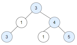
Input: root = [3,1,4,3,null,1,5] Output: 4 Explanation: Nodes in blue are good. Root Node (3) is always a good node. Node 4 -> (3,4) is the maximum value in the path starting from the root. Node 5 -> (3,4,5) is the maximum value in the path Node 3 -> (3,1,3) is the maximum value in the path.
Example 2:
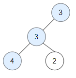
Input: root = [3,3,null,4,2] Output: 3 Explanation: Node 2 -> (3, 3, 2) is not good, because "3" is higher than it.
Example 3:
Input: root = [1] Output: 1 Explanation: Root is considered as good.
Constraints:
- The number of nodes in the binary tree is in the range
[1, 10^5]. - Each node’s value is between
[-10^4, 10^4].
※ 2.8.11.1. Constraints and Edge Cases
- no empty trees will be given, at least will have one good node
※ 2.8.11.2. My Solution (Code)
※ 2.8.11.2.1. Iterative BFS, keep max_above for each node
This is a BFS
1: from collections import deque 2: 3: class Solution: 4: │ def goodNodes(self, root: TreeNode) -> int: 5: │ │ queue = deque([(root, -float('inf'))]) # node, keep max above itself 6: │ │ count = 0 7: │ │ while queue: 8: │ │ │ # get the level: 9: │ │ │ # evaluate current 10: │ │ │ for _ in range(len(queue)): 11: │ │ │ │ node, max_above = queue.popleft() 12: │ │ │ │ 13: │ │ │ │ if node.val >= max_above: 14: │ │ │ │ │ # only need to update max_above in this case: 15: │ │ │ │ │ max_above = max(max_above, node.val) 16: │ │ │ │ │ count += 1 17: │ │ │ │ │ 18: │ │ │ │ │ 19: │ │ │ │ # add children: 20: │ │ │ │ if node.left: 21: │ │ │ │ │ queue.append((node.left, max_above)) 22: │ │ │ │ if node.right: 23: │ │ │ │ │ queue.append((node.right, max_above)) 24: │ │ │ │ │ 25: │ │ return count
Technically we don’t really need to do the level by level.
- You don’t need the inner
for _ in range(len(queue)):loop unless you’re specifically processing level by level. For this problem, a simplewhile queue:loop suffices. No need to update
max_aboveonly when the node is good; always update it tomax(max_above, node.val)for the children.this is a cleanup of the BFS solution:
1: from collections import deque 2: 3: class Solution: 4: │ def goodNodes(self, root: TreeNode) -> int: 5: │ │ queue = deque([(root, root.val)]) 6: │ │ count = 0 7: │ │ while queue: 8: │ │ │ node, max_above = queue.popleft() 9: │ │ │ if node.val >= max_above: 10: │ │ │ │ count += 1 11: │ │ │ max_new = max(max_above, node.val) 12: │ │ │ if node.left: 13: │ │ │ │ queue.append((node.left, max_new)) 14: │ │ │ if node.right: 15: │ │ │ │ queue.append((node.right, max_new)) 16: │ │ return count
※ 2.8.11.2.2. Canonical Optimal Solution (DFS)
here’s the recursive canonical: it uses the state threading as well, since the level data is passed via the arguments. however, I found this slow
1: class Solution: 2: │ def goodNodes(self, root: TreeNode) -> int: 3: │ │ def dfs(node, max_above): 4: │ │ │ if not node: 5: │ │ │ │ return 0 6: │ │ │ │ 7: │ │ │ good = 1 if node.val >= max_above else 0 8: │ │ │ max_new = max(max_above, node.val) 9: │ │ │ 10: │ │ │ return good + dfs(node.left, max_new) + dfs(node.right, max_new) 11: │ │ │ 12: │ │ return dfs(root, float('-inf'))
here’s the iterative DFS:
1: class Solution: 2: │ def goodNodes(self, root: TreeNode) -> int: 3: │ │ if not root: 4: │ │ │ return 0 5: │ │ │ 6: │ │ stack = [(root, root.val)] # Each entry: (node, max_above) 7: │ │ count = 0 8: │ │ 9: │ │ while stack: 10: │ │ │ node, max_above = stack.pop() 11: │ │ │ if node.val >= max_above: 12: │ │ │ │ count += 1 13: │ │ │ max_new = max(max_above, node.val) 14: │ │ │ # Push children with updated max_above 15: │ │ │ if node.left: 16: │ │ │ │ stack.append((node.left, max_new)) 17: │ │ │ if node.right: 18: │ │ │ │ stack.append((node.right, max_new)) 19: │ │ │ │ 20: │ │ return count
Key points:
- The stack holds tuples of
(node, max_above), so each node knows the maximum value on its path from the root. - For each node, check if it’s “good” (node.val >=
max_above). If so, increment the count. - Always update
max_abovefor children asmax(max_above, node.val)—this is the correct max for their path, regardless of whether the parent is “good”
This approach avoids recursion depth issues and is efficient for large/deep trees
- The stack holds tuples of
※ 2.8.11.3. My Approach/Explanation
- I need to keep track of the max aboves for each node. So what do is that each time I actually keep track of the max above
※ 2.8.11.4. My Learnings/Questions
- Intuition: The key insight is to thread the “max value seen so far” along the path, so you can check each node in \(O(1)\) time.
- I’m happy that I can augment things as I wish. The main thing here is to be clear about what the “processed and unprocessed” parts are. In this case, it’s by design that the max is “max above this node” because we haven’t really processed this node until we pop it out of the stack.
※ 2.8.11.5. [Optional] Additional Context
I am SPEED 🏎️
※ 2.8.12. [55] Validate Binary Search Tree (98) bst_property
Given the root of a binary tree, determine if it is a valid binary
search tree (BST).
A valid BST is defined as follows:
- The left subtree of a node contains only nodes with keys less than the node’s key.
- The right subtree of a node contains only nodes with keys greater than the node’s key.
- Both the left and right subtrees must also be binary search trees.
Example 1:

Input: root = [2,1,3] Output: true
Example 2:

Input: root = [5,1,4,null,null,3,6] Output: false Explanation: The root node's value is 5 but its right child's value is 4.
Constraints:
- The number of nodes in the tree is in the range
[1, 10=^{=4}=]=. -2=^{=31}= <= Node.val <= 2=31= - 1=
※ 2.8.12.1. Constraints and Edge Cases
- needs to not just consider parent but the range above the parent. The “context” has to be large enough
※ 2.8.12.2. My Solution (Code)
※ 2.8.12.2.1. Correct Solution:
1: from collections import deque 2: class Solution: 3: │ def isValidBST(self, root: Optional[TreeNode]) -> bool: 4: │ │ queue = deque([(root, -float('inf'), float('inf'))]) # node, lower and upper 5: │ │ 6: │ │ while queue: 7: │ │ │ # exclusive bounds 8: │ │ │ node, lower, upper = queue.popleft() 9: │ │ │ 10: │ │ │ if not node: 11: │ │ │ │ continue 12: │ │ │ │ 13: │ │ │ if node.val >= upper or node.val <= lower: 14: │ │ │ │ return False 15: │ │ │ │ 16: │ │ │ if node.left: 17: │ │ │ │ # constricts left, so new upper = node.val 18: │ │ │ │ queue.append((node.left, lower, node.val)) 19: │ │ │ if node.right: 20: │ │ │ │ # constricts right, so new lower = node.val 21: │ │ │ │ queue.append((node.right, node.val, upper)) 22: │ │ │ │ 23: │ │ return True
Alternatively, here’s a Recursive version:
1: class Solution: 2: │ def isValidBST(self, root: Optional[TreeNode]) -> bool: 3: │ │ def validate(node, lower, upper): 4: │ │ │ if not node: 5: │ │ │ │ return True 6: │ │ │ │ 7: │ │ │ if not (lower < node.val < upper): 8: │ │ │ │ return False 9: │ │ │ │ 10: │ │ │ return (validate(node.left, lower, node.val) and 11: │ │ │ │ │ validate(node.right, node.val, upper)) 12: │ │ │ │ │ 13: │ │ return validate(root, float('-inf'), float('inf')) 14:
Correct idea, wrong execution
1: # Definition for a binary tree node. 2: # class TreeNode: 3: # def __init__(self, val=0, left=None, right=None): 4: # self.val = val 5: # self.left = left 6: # self.right = right 7: from collections import deque 8: class Solution: 9: │ def isValidBST(self, root: Optional[TreeNode]) -> bool: 10: │ │ queue = deque([(root, -float('inf'), float('inf'))]) # node, left max (can't be more than this), right min (can't be less than that) 11: │ │ while queue: 12: │ │ │ node, left_max, right_min = queue.popleft() 13: │ │ │ 14: │ │ │ if not node: 15: │ │ │ │ continue 16: │ │ │ │ 17: │ │ │ if node.val > left_max or node.val < right_min: 18: │ │ │ │ return False 19: │ │ │ │ # can continue: 20: │ │ │ if node.left: 21: │ │ │ │ queue.append((node.left, min(node.val, left_max), max(node.val, right_min))) 22: │ │ │ if node.right: 23: │ │ │ │ queue.append((node.right, min(node.val, left_max), max(node.val, right_min))) 24: │ │ │ │ 25: │ │ return True
Problems:
- messy naming \(\implies\) messy logic. It should just have been named
(low, high)or something since we’re keeping track of bounds. - The root node should have no bounds: use
-infand+infas initial limits. - the bounds should be for “everything above this node”
※ 2.8.12.2.2. Alternative Working Approach: Inorder Check:
Use BST inorder traversal (which is sorted)
Inorder Traversal (Iterative or Recursive)
In a valid BST, the inorder traversal yields a strictly increasing sequence.
You can traverse in-order and check that each value is greater than the previous.
Show/Hide Python Code1: class Solution: 2: │ def isValidBST(self, root: Optional[TreeNode]) -> bool: 3: │ │ stack, prev = [], None 4: │ │ while stack or root: 5: │ │ │ while root: 6: │ │ │ │ stack.append(root) 7: │ │ │ │ root = root.left 8: │ │ │ root = stack.pop() 9: │ │ │ if prev is not None and root.val <= prev: 10: │ │ │ │ return False 11: │ │ │ prev = root.val 12: │ │ │ root = root.right 13: │ │ return True 14:
※ 2.8.12.2.3. Faulty (logically flawed version)
This will actually pass some test cases, but it has a flaw whereby we only look at the immediate parent, which is not enough, so this will false positive cases where we actually have deeper, skewed substrees with violating nodes but we won’t catch them because our “context” only includes what is at the immediate parent.
1: class Solution: 2: │ def isValidBST(self, root: Optional[TreeNode]) -> bool: 3: │ │ def bfs(root, left, right): 4: │ │ │ if not root: 5: │ │ │ │ return True 6: │ │ │ if root.val < left or root.val > right: 7: │ │ │ │ return False 8: │ │ │ │ 9: │ │ │ if root.left: 10: │ │ │ │ # right is constricted now: 11: │ │ │ │ if not bfs(root.left, left, root.val): 12: │ │ │ │ │ return False 13: │ │ │ │ │ 14: │ │ │ if root.right: 15: │ │ │ │ # left is constricted now: 16: │ │ │ │ if not bfs(root.right, root.val, right): 17: │ │ │ │ │ return False 18: │ │ │ │ │ 19: │ │ │ return True 20: │ │ │ 21: │ │ bfs(root, -float('inf'), float('inf')) 22: │ │ 23: │ │ return True 24:
This won’t work because can’t just keep the context of the immediate parent, need to keep the context of everything above it
※ 2.8.12.3. My Approach/Explanation
My initial approach was flawed because the amount of “context” I had was limited to just the parent. This is not enough, so this will false positive cases where we actually have deeper, skewed substrees with violating nodes but we won’t catch them because our “context” only includes what is at the immediate parent.
So there’s a need to keep the context of “above this node” again, which is what we need to add in. Specifically, we need to keep track of boundaries (lower, upper). In this case, we’re using strict boundaries.
※ 2.8.12.4. My Learnings/Questions
- Python supports chained comparison: so
lower < test < upperwill work- this operation is lazy
- this only evaluates the
testonce and breaks it down into(lower < test) and (test < upper)
- once again, we’re keeping track of “everything above this node” / visited / processed history context. I think this analogy of “what’s the context we need to keep for the encountered incidents we’ve seen so far” is helpful to me to determine how I should be handling the annotation / augmentation part.
- The completely different approach involves using the BST property of the ordering and do an in-order-traversal. If values are in sorted order, then it’s a valid BST!
※ 2.8.13. [56] Kth Smallest Element in BST (230) augmentation
Given the root of a binary search tree, and an integer k, return
the k=^{=th} smallest value (1-indexed) of all the values of the
nodes in the tree.
Example 1:
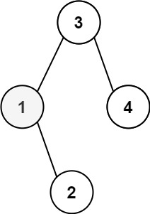
Input: root = [3,1,4,null,2], k = 1 Output: 1
Example 2:
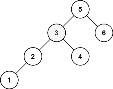
Input: root = [5,3,6,2,4,null,null,1], k = 3 Output: 3
Constraints:
- The number of nodes in the tree is
n. 1 <k <= n <= 10=40 <Node.val <= 10=4
Follow up: If the BST is modified often (i.e., we can do insert and delete operations) and you need to find the kth smallest frequently, how would you optimize?
※ 2.8.13.1. Constraints and Edge Cases
<list constraints, input limits, or tricky edge cases here>
※ 2.8.13.2. My Solution (Code)
※ 2.8.13.2.1. BST In-Order Traversal
1: class Solution: 2: │ def kthSmallest(self, root: Optional[TreeNode], k: int) -> int: 3: │ │ stack = [root] 4: │ │ curr = root 5: │ │ while stack or curr: 6: │ │ │ # go as left as possible, keep adding to the stack: 7: │ │ │ while curr: 8: │ │ │ │ stack.append(curr) 9: │ │ │ │ curr = curr.left 10: │ │ │ │ 11: │ │ │ # process node, get from the stack: 12: │ │ │ curr = stack.pop() 13: │ │ │ k -= 1 14: │ │ │ 15: │ │ │ if k == 0: 16: │ │ │ │ return curr.val 17: │ │ │ │ 18: │ │ │ # go right subtree 19: │ │ │ curr = curr.right
1: class Solution: 2: │ def kthSmallest(self, root: Optional[TreeNode], k: int) -> int: 3: │ │ self.k = k 4: │ │ self.res = None 5: │ │ 6: │ │ def inorder(node): 7: │ │ │ if not node or self.res is not None: 8: │ │ │ │ return 9: │ │ │ │ 10: │ │ │ # left recurse 11: │ │ │ inorder(node.left) 12: │ │ │ 13: │ │ │ # handle this node 14: │ │ │ self.k -= 1 15: │ │ │ if self.k == 0: 16: │ │ │ │ self.res = node.val 17: │ │ │ │ return 18: │ │ │ │ 19: │ │ │ # handle right 20: │ │ │ inorder(node.right) 21: │ │ │ 22: │ │ inorder(root) 23: │ │ 24: │ │ return self.res
※ 2.8.13.2.2. Inefficient but works for frequent modifications
I was biased because of the extensions prompt.
I wanted to keep a min-queue as an auxiliary.
NOTE: this isn’t the best way to do things, it just keeps the access at \(O(1)\) despite frequent modifications.
1: import heapq 2: 3: class Solution: 4: │ def kthSmallest(self, root: Optional[TreeNode], k: int) -> int: 5: │ │ queue = [] # min queue 6: │ │ stack = [root] 7: │ │ 8: │ │ while stack: 9: │ │ │ node = stack.pop() 10: │ │ │ heapq.heappush(queue, (node.val, node)) 11: │ │ │ 12: │ │ │ if node.left: 13: │ │ │ │ stack.append(node.left) 14: │ │ │ if node.right: 15: │ │ │ │ stack.append(node.right) 16: │ │ │ │ 17: │ │ return heapq.nsmallest(k, queue)[-1][0] 18:
We can get accesses quickly because of this, and once updated, it’s easy to maintain.
- Here’s why this access pattern is necessary, based on the heapq API:
heapq.nsmallest(k, queue)returns a list of the k smallest elements from queue, sorted in ascending order by their value- Since queue contains tuples like
(node.val, node), the smallest elements are determined by node.val. - The returned list has the
ksmallest tuples, so[-1]accesses the \(k^{th}\) smallest tuple (because the list is sorted: index 0 is the smallest, indexk-1is the \(k^{th}\) smallest)
※ 2.8.13.3. My Approach/Explanation
Here we exploit BST property in that an in-order traversal will give elements from the BST in sorted order. We can just keep a count and do the in-order traversal.
※ 2.8.13.4. My Learnings/Questions
- this is one of the few times I tried an iterative inorder DFS implementation. The idea is to add in a separate while loop so that our consideration stack (the stack) is filled as LEFT as possible. This allows us to do the left then middle then right (in-order) traversal that we want to do.
- It’s a nifty trick here that the
kis being used as the counter itself. QQ: Is my suggestion to the extension question accurate? or is it more of ’addition to BST is in \(O(1)\) time so we can just modify an array’ or something like that?
AA: nope, they expect the answer to be more of an augmentation of the existing tree.
Heap is not the best for a BST: Maintaining a heap for all values allows O(1) kth smallest access but O(N) update time for insert/delete.
Augmented BST is preferred: For frequent modifications and kth smallest queries, augment the BST with subtree sizes. This allows both updates and queries in O(H) time
Use an augmented BST where each node stores the size of its left subtree (
lCount). This allows \(O(H)\) time for \(k^{th}\) smallest queries and \(O(H)\) time for updates- Augmented BST for Frequent Modifications
- Each node keeps track of the size of its left subtree.
- When you insert or delete, you update the counts.
- To find \(k^{th}\) smallest:
- If
k =lCount + 1=, return node. - If k <= lCount, go left.
- Else, go right with
k - lCount - 1
- If
- Augmented BST for Frequent Modifications
※ 2.8.14. [57] ⭐️ Construct Binary Tree from Preorder and Inorder Traversal (105) redo traversal_properties
Given two integer arrays preorder and inorder where preorder is
the preorder traversal of a binary tree and inorder is the inorder
traversal of the same tree, construct and return the binary tree.
Example 1:
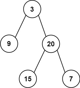
Input: preorder = [3,9,20,15,7], inorder = [9,3,15,20,7] Output: [3,9,20,null,null,15,7]
Example 2:
Input: preorder = [-1], inorder = [-1] Output: [-1]
Constraints:
1 <preorder.length <= 3000=inorder.length =preorder.length=-3000 <preorder[i], inorder[i] <= 3000=preorderandinorderconsist of unique values.- Each value of
inorderalso appears inpreorder. preorderis guaranteed to be the preorder traversal of the tree.inorderis guaranteed to be the inorder traversal of the tree.
※ 2.8.14.1. Constraints and Edge Cases
- no empty case to handle
- most of the typical edge cases aren’t relevant because of the constraints given.
※ 2.8.14.2. My Solution (Code)
I couldn’t get this myself because of the key insight:
- inorder traversal can help us partition the left and right subtree nodes
※ 2.8.14.2.1. Guided Optimal Solution
1: class Solution: 2: │ def buildTree(self, preorder: List[int], inorder: List[int]) -> Optional[TreeNode]: 3: │ │ 4: │ │ inorder_val_to_idx = {val:idx for idx, val in enumerate(inorder)} 5: │ │ pre_idx = 0 6: │ │ 7: │ │ def helper(left, right): 8: │ │ │ nonlocal pre_idx 9: │ │ │ 10: │ │ │ if left > right: 11: │ │ │ │ return None 12: │ │ │ root_val = preorder[pre_idx] 13: │ │ │ root = TreeNode(val=root_val) 14: │ │ │ pre_idx += 1 15: │ │ │ inorder_idx = inorder_val_to_idx[root_val] 16: │ │ │ root.left = helper(left, inorder_idx - 1) 17: │ │ │ root.right = helper(inorder_idx + 1, right) 18: │ │ │ 19: │ │ │ return root 20: │ │ │ 21: │ │ return helper(0, len(inorder) - 1)
- Time Complexity:
- Each node is processed once, and the index lookup in the hashmap is \(O(1)\).
- Total: \(O(N)\), where N is the number of nodes.
- Space Complexity:
- The hashmap takes \(O(N)\) space.
- The recursion stack takes \(O(H)\) space (\(H\) = height of the tree, up to \(O(N)\) if the tree is skewed).
- Total: \(O(N)\).
Here’s a formatted one, should be cleaner:
1: class Solution: 2: │ def buildTree(self, preorder: List[int], inorder: List[int]) -> Optional[TreeNode]: 3: │ │ idx_map = {val: i for i, val in enumerate(inorder)} 4: │ │ preorder_index = 0 5: │ │ 6: │ │ def helper(left, right): 7: │ │ │ nonlocal preorder_index 8: │ │ │ if left > right: 9: │ │ │ │ return None 10: │ │ │ │ 11: │ │ │ root_val = preorder[preorder_index] 12: │ │ │ preorder_index += 1 13: │ │ │ root = TreeNode(root_val) 14: │ │ │ 15: │ │ │ # Build left and right subtrees 16: │ │ │ root.left = helper(left, idx_map[root_val] - 1) 17: │ │ │ root.right = helper(idx_map[root_val] + 1, right) 18: │ │ │ return root 19: │ │ │ 20: │ │ return helper(0, len(inorder) - 1)
※ 2.8.14.2.2. Optimised Solution: with generators
Using a generator for the preorder traversal eliminates manual index management, avoids inefficient list operations, and results in cleaner, more idiomatic code — while maintaining optimal time and space complexity.
1: class Solution: 2: │ def buildTree(self, preorder: List[int], inorder: List[int]) -> Optional[TreeNode]: 3: │ │ inorder_val_to_idx = {val: idx for idx, val in enumerate(inorder)} 4: │ │ preorder_iter = iter(preorder) # Create a generator from preorder 5: │ │ 6: │ │ def helper(left, right): 7: │ │ │ if left > right: 8: │ │ │ │ return None 9: │ │ │ │ 10: │ │ │ root_val = next(preorder_iter) # Get the next root value from the generator 11: │ │ │ root = TreeNode(root_val) 12: │ │ │ inorder_idx = inorder_val_to_idx[root_val] 13: │ │ │ root.left = helper(left, inorder_idx - 1) 14: │ │ │ root.right = helper(inorder_idx + 1, right) 15: │ │ │ 16: │ │ │ return root 17: │ │ │ 18: │ │ return helper(0, len(inorder) - 1) 19:
The generator yields the next root value for each subtree in preorder, so you never have to manage the index yourself.
This makes the code cleaner and avoids side effects (like modifying the input list).
Why is this an improvement?
No need for nonlocal or global index variables: The generator maintains its own state.
No mutation of input list: Unlike pop(0), which is \(O(N)\) per operation, or slicing, which is also inefficient, next() on a generator is \(O(1)\).
Cleaner, more idiomatic Python: The code is easier to read and reason about.
※ 2.8.14.3. My Approach/Explanation
See learnings below
※ 2.8.14.4. My Learnings/Questions
- Intuition: The key insight is that the preorder sequence gives you the root, and the inorder sequence tells you how to split the tree. Recursively applying this builds the tree efficiently.
- I couldn’t do this so here’s some write ups.
- We should first consider the properties of the traversals:
- Preorder: the first element is always the root of the current subtree
- Inorder: the index of the root splits the array into left and right subtrees
- Algo:
- We use the first value in pre-order as the root
- Find the index of this root in inorder:
- elements to the left of this idx are the left subtree, right are the right subtree
- repeat recursively for the subtrees
- We should first consider the properties of the traversals:
Python Scopes: QQ: why is it that for the generator approach, we don’t need to use a
nonlocal?AA: It’s because of the difference between accessing vs assigning variables
Reading a variable from an enclosing scope? No
nonlocalneeded.Assigning to a variable from an enclosing scope? You must declare it as
nonlocal.see the long form answer below:
Show/Hide Md CodeThe reason you **do not** need to declare `preorder_iter` as `nonlocal` inside the `helper` function, while you **do** need to declare a variable like `pre_idx` as `nonlocal`, comes down to **how Python handles variable lookup and assignment in nested scopes** (the LEGB rule)[3][5][6][7]: ### **Accessing vs. Assigning Variables** - **Accessing (Reading):** │ If you only *read* a variable from an enclosing scope (like `preorder_iter`), Python will look for it in the local scope, then the enclosing scope, then global, then built-in (LEGB rule). You do **not** need to declare it as `nonlocal` or `global` if you are only reading it[3][5][7]. │ - **Assigning (Writing):** │ If you *assign* to a variable (e.g., `pre_idx += 1`), Python treats it as a **new local variable** unless you explicitly declare it as `nonlocal` (for enclosing function scope) or `global` (for module scope)[3][5][7]. │ This is why you need `nonlocal pre_idx` if you want to update the value from the enclosing scope. │ ### **Why the Generator (`preorder_iter`) Works Without `nonlocal`** - In the generator-based solution, you only *call* `next(preorder_iter)` inside `helper`. You are **not assigning** to `preorder_iter` inside `helper`; you are only *using* it (reading its value). - Since there is no assignment, Python simply looks up `preorder_iter` in the enclosing scope and uses it[3][5][7]. ### **Why an Index Variable Needs `nonlocal`** - If you use an index variable like `pre_idx` and want to increment it (`pre_idx += 1`), you are *assigning* to it. - Without `nonlocal`, Python would treat `pre_idx` as a new local variable inside `helper`, which is not what you want. - Declaring `nonlocal pre_idx` tells Python to use the variable from the enclosing (outer) function scope[3][5][7]. ### **Summary Table** | Variable Type | Only Read? | Assigned? | Needs `nonlocal`? | |-------------------|------------|-----------|-------------------| | Generator object | Yes | No | No | | Index variable | No | Yes | Yes | **References:** - [RealPython: LEGB Rule][3] - [ZetCode: Variable Scope][5] - [TutorialsPoint: Scoping Rules][6] - [Codefinity: LEGB Rule][7] **In short:** - **Reading** a variable from an enclosing scope? No `nonlocal` needed. - **Assigning** to a variable from an enclosing scope? You **must** declare it as `nonlocal`. Let me know if you want a code example to illustrate this! [1] https://www.w3schools.com/python/python_scope.asp [2] https://www.datacamp.com/tutorial/scope-of-variables-python [3] https://realpython.com/python-scope-legb-rule/ [4] https://stackoverflow.com/questions/291978/short-description-of-the-scoping-rules [5] https://zetcode.com/python/variable-scope/ [6] https://www.tutorialspoint.com/what-are-the-basic-scoping-rules-for-python-variables [7] https://codefinity.com/blog/Understanding-Scopes-in-Python-and-the-LEGB-Rule [8] https://docs.python.org/3/tutorial/classes.html [9] https://labex.io/tutorials/python-how-to-manage-python-scope-rules-421901 [10] https://stackoverflow.com/questions/23940956/variable-scope-in-a-python-generator-expression
- comments on pythonic style:
- Using a hashmap for \(O(1)\) index lookup is the key improvement over naive approaches.
- Use of
nonlocalis idiomatic for tracking the preorder index. - No need to slice arrays (which would be \(O(N^{2})\) in Python).
- If you want, you could use a generator for preorder traversal, but your approach is already optimal and clear.
- You can reconstruct a tree from preorder + inorder, or postorder + inorder, but not from preorder + postorder alone (unless the tree is full).
※ 2.8.15. [58] Binary Tree Maximum Path Sum (124) redo hard gain_accumulation
A path in a binary tree is a sequence of nodes where each pair of adjacent nodes in the sequence has an edge connecting them. A node can only appear in the sequence at most once. Note that the path does not need to pass through the root.
The path sum of a path is the sum of the node’s values in the path.
Given the root of a binary tree, return the maximum path sum of any
non-empty path.
Example 1:
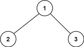
Input: root = [1,2,3] Output: 6 Explanation: The optimal path is 2 -> 1 -> 3 with a path sum of 2 + 1 + 3 = 6.
Example 2:
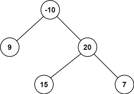
Input: root = [-10,9,20,null,null,15,7] Output: 42 Explanation: The optimal path is 15 -> 20 -> 7 with a path sum of 15 + 20 + 7 = 42.
Constraints:
- The number of nodes in the tree is in the range
[1, 3 * 10=^{=4}=]=. -1000 <Node.val <= 1000=
※ 2.8.15.1. Constraints and Edge Cases
Nothing fancy here
※ 2.8.15.2. My Solution (Code)
※ 2.8.15.2.1. My attempt
1: class Solution: 2: │ def maxPathSum(self, root: Optional[TreeNode]) -> int: 3: │ │ if not root.left and not root.right: 4: │ │ │ return root.val 5: │ │ │ 6: │ │ # if inputs can be negative then this should be max negative 7: │ │ max_sum = float(-inf) 8: │ │ 9: │ │ # returns from this node and choosing one side from this 10: │ │ def dfs(root: Optional[TreeNode]): 11: │ │ │ nonlocal max_sum 12: │ │ │ 13: │ │ │ if root is None: 14: │ │ │ │ return 0 15: │ │ │ │ 16: │ │ │ # only consider +ve contributions, if negative, take 0 17: │ │ │ max_left = max(dfs(root.left), 0) 18: │ │ │ max_right = max(dfs(root.right), 0) 19: │ │ │ 20: │ │ │ # for the case where pass passes through this node: 21: │ │ │ max_sum = max(max_sum, max_left + max_right + root.val) 22: │ │ │ 23: │ │ │ # return max gain if continuing the same path upwards 24: │ │ │ # have to choose b/w right or left subtree as path: 25: │ │ │ best_choice = max(max_left, max_right) 26: │ │ │ return root.val + best_choice 27: │ │ │ 28: │ │ dfs(root) 29: │ │ 30: │ │ return max_sum
Here’s another cleaned up version from the bot:
1: class Solution: 2: │ def maxPathSum(self, root: Optional[TreeNode]) -> int: 3: │ │ max_sum = float('-inf') 4: │ │ 5: │ │ def dfs(node): 6: │ │ │ nonlocal max_sum 7: │ │ │ if not node: 8: │ │ │ │ return 0 9: │ │ │ # Ignore negative branches 10: │ │ │ left_gain = max(dfs(node.left), 0) 11: │ │ │ right_gain = max(dfs(node.right), 0) 12: │ │ │ # Max path sum WITH split at this node 13: │ │ │ price_newpath = node.val + left_gain + right_gain 14: │ │ │ max_sum = max(max_sum, price_newpath) 15: │ │ │ # Return max gain for parent (must pick one branch) 16: │ │ │ return node.val + max(left_gain, right_gain) 17: │ │ │ 18: │ │ dfs(root) 19: │ │ return max_sum
Here’s a state-threaded version:
1: from typing import Optional, Tuple 2: 3: class Solution: 4: │ def maxPathSum(self, root: Optional['TreeNode']) -> int: 5: │ │ 6: │ │ def dfs(node: Optional['TreeNode'], current_max: int) -> Tuple[int, int]: 7: │ │ │ # Returns (max_gain_upwards, max_path_sum_so_far) 8: │ │ │ if not node: 9: │ │ │ │ # max gain upwards = 0, max path sum so far = current max unchanged 10: │ │ │ │ return 0, current_max 11: │ │ │ │ 12: │ │ │ left_gain, current_max = dfs(node.left, current_max) 13: │ │ │ right_gain, current_max = dfs(node.right, current_max) 14: │ │ │ 15: │ │ │ left_gain = max(left_gain, 0) 16: │ │ │ right_gain = max(right_gain, 0) 17: │ │ │ 18: │ │ │ price_newpath = node.val + left_gain + right_gain 19: │ │ │ current_max = max(current_max, price_newpath) 20: │ │ │ 21: │ │ │ max_gain_upwards = node.val + max(left_gain, right_gain) 22: │ │ │ 23: │ │ │ return max_gain_upwards, current_max 24: │ │ │ 25: │ │ _, max_sum = dfs(root, float('-inf')) 26: │ │ return max_sum
The idea is kinda right, the depth in thinking really not there anymore lmao.
Problems:
need to figure out what the return value from the DFS should be:
The value you return from dfs should represent the maximum path sum starting from this node and going down ONE side only (either left or right, or just the node itself).
Why?
Because a path cannot split as it ascends to the parent (otherwise, the path would fork, which is not allowed).
updating the accumulating var (
max_sum)You should update
max_sumwith the maximum path sum passing through the current node (which can include both children), but when returning, you can only pass up one side.You are updating
max_sumwithmax_left, max_right, and max_left + max_right + root.val,but not considering the possibility that the best path may be just the node itself or node + one side.If negative inputs possible, init the accumulator var to max int that is negative!
Your
max_sumis initialized to 0.If all node values are negative, you will return 0 instead of the correct maximum (which should be the least negative node).
You should initialize
max_sumto-inf
1: class Solution: 2: │ def maxPathSum(self, root: Optional[TreeNode]) -> int: 3: │ │ if not root.left and not root.right: 4: │ │ │ return root.val 5: │ │ │ 6: │ │ max_sum = 0 7: │ │ 8: │ │ def dfs(root: Optional[TreeNode]): 9: │ │ │ nonlocal max_sum 10: │ │ │ 11: │ │ │ if root is None: 12: │ │ │ │ return 0 13: │ │ │ │ 14: │ │ │ max_left = dfs(root.left) 15: │ │ │ max_right = dfs(root.right) 16: │ │ │ 17: │ │ │ max_sum = max(max_sum, max_left, max_right, max_left + max_right + root.val) 18: │ │ │ combined = max_left + max_right + root.val 19: │ │ │ 20: │ │ │ max_sum = max(max_sum, combined) 21: │ │ │ 22: │ │ │ return combined 23: │ │ │ 24: │ │ dfs(root) 25: │ │ 26: │ │ return max_sum
※ 2.8.15.3. My Approach/Explanation
- The return value from dfs should represent the max gain from this node up one branch.
- Update
max_sumwith the sum ofleft + right + node.valat each node. - Always initialize
max_sumto negative infinity to handle negative values correctly.
※ 2.8.15.4. My Learnings/Questions
- Key Intuition:
- The key is realizing that the return value of DFS is the best single-branch gain, while the global update considers the sum through both children and the current node.
All optimal solutions use post-order DFS, since you need to know the best gain from both children before computing the answer for the current node.
You could use an explicit stack for iterative post-order traversal, but it is more complex and rarely used for this problem.
- The mental model of “max gain” is important here. We are walking up the tree and we know that:
- we have to get the “best gain” if it’s
L_SUBTREE + THIS NODE + RIGHT_SUBTREE - to continue walking up, it’s going to be either:
THIS_NODE + LEFT_SUBTREE- OR,
THIS_NODE + RIGHT_SUBTREE - OR,
THIS_NODE
- we have to get the “best gain” if it’s
※ 2.8.15.5. [Optional] Additional Context
I realise that at the end of the day, I’m genuinely tired to the point that I can’t think straight.
I should switch to other tasks when I hit this wall and resume fresh the next morning.
※ 2.8.16. TODO [59] Serialize and Deeserialize Binary Tree (297) redo hard backtracking trie
Serialization is the process of converting a data structure or object into a sequence of bits so that it can be stored in a file or memory buffer, or transmitted across a network connection link to be reconstructed later in the same or another computer environment.
Design an algorithm to serialize and deserialize a binary tree. There is no restriction on how your serialization/deserialization algorithm should work. You just need to ensure that a binary tree can be serialized to a string and this string can be deserialized to the original tree structure.
Clarification: The input/output format is the same as how LeetCode serializes a binary tree. You do not necessarily need to follow this format, so please be creative and come up with different approaches yourself.
Example 1:
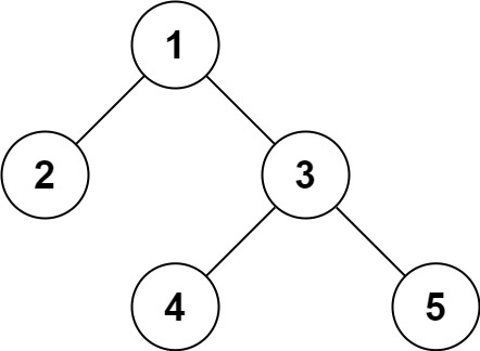
Input: root = [1,2,3,null,null,4,5] Output: [1,2,3,null,null,4,5]
Example 2:
Input: root = [] Output: []
Constraints:
- The number of nodes in the tree is in the range
[0, 10=^{=4}=]=. -1000 <Node.val <= 1000=
※ 2.8.16.1. Constraints and Edge Cases
<list constraints, input limits, or tricky edge cases here>
※ 2.8.16.2. My Solution (Code)
※ 2.8.16.2.1. Optimal Solution
1: # Definition for a binary tree node. 2: # class TreeNode(object): 3: # def __init__(self, x): 4: # self.val = x 5: # self.left = None 6: # self.right = None 7: 8: from collections import deque 9: 10: class Codec: 11: │ 12: │ def serialize(self, root): 13: │ │ """Encodes a tree to a single string. 14: │ │ 15: │ │ :type root: TreeNode 16: │ │ :rtype: str 17: │ │ """ 18: │ │ if not root: 19: │ │ │ return "null" 20: │ │ │ 21: │ │ result = [] 22: │ │ queue = deque([root]) 23: │ │ while queue: 24: │ │ │ node = queue.popleft() 25: │ │ │ if node: 26: │ │ │ │ result.append(str(node.val)) 27: │ │ │ │ queue.append(node.left) 28: │ │ │ │ queue.append(node.right) 29: │ │ │ else: 30: │ │ │ │ result.append("null") 31: │ │ │ │ 32: │ │ # trim trailing nulls, help to reduce size since trailing nulls unncessary 33: │ │ while result and result[-1] == "null": 34: │ │ │ result.pop() 35: │ │ │ 36: │ │ return ",".join(result) 37: │ │ 38: │ def deserialize(self, data): 39: │ │ """Decodes your encoded data to tree. 40: │ │ 41: │ │ :type data: str 42: │ │ :rtype: TreeNode 43: │ │ """ 44: │ │ if data == "null": 45: │ │ │ return None 46: │ │ │ 47: │ │ nodes = data.split(",") 48: │ │ root = TreeNode(int(nodes[0])) 49: │ │ queue = deque([root]) 50: │ │ idx = 1 51: │ │ while queue: 52: │ │ │ node = queue.popleft() 53: │ │ │ if idx < len(nodes): 54: │ │ │ │ if nodes[idx] != "null": 55: │ │ │ │ │ node.left = TreeNode(int(nodes[idx])) 56: │ │ │ │ │ queue.append(node.left) 57: │ │ │ │ idx += 1 58: │ │ │ │ 59: │ │ │ if idx < len(nodes): 60: │ │ │ │ if nodes[idx] != "null": 61: │ │ │ │ │ node.right = TreeNode(int(nodes[idx])) 62: │ │ │ │ │ queue.append(node.right) 63: │ │ │ │ idx += 1 64: │ │ │ │ 65: │ │ return root
※ 2.8.16.2.2. Tapped out
I feel like I dug a hole because of how complex I made it. My approach was to go level order, remembering to:
- keep left padding
- keep right padding
serialising current
Show/Hide Python Code1: from collections import deque 2: 3: class Codec: 4: │ 5: │ def serialize(self, root): 6: │ │ """Encodes a tree to a single string. 7: │ │ 8: │ │ :type root: TreeNode 9: │ │ :rtype: str 10: │ │ """ 11: │ │ queue = deque([root, 0, False]) # node, parent_level_idx, is_right 12: │ │ serial = [] 13: │ │ 14: │ │ level = 0 15: │ │ while queue: 16: │ │ │ # iterate thru the level: 17: │ │ │ level_cap = 2**level 18: │ │ │ 19: │ │ │ # keep left padding: 20: │ │ │ _, first_parent_idx, first_is_right = queue[0] 21: │ │ │ left_padding = [] 22: │ │ │ if first_parent_idx > 0: # need padding: 23: │ │ │ │ left_padding.extend(("null" for idx in range(first_parent_idx))) 24: │ │ │ │ 25: │ │ │ # keep right padding: 26: │ │ │ _, last_parent_idx, last_is_right = queue[-1] 27: │ │ │ 28: │ │ │ 29: │ │ │ 30: │ │ │ 31: │ │ │ 32: │ │ │ # now the mids: 33: │ │ │ middle = [] 34: │ │ │ for _ in range(len(queue)): 35: │ │ │ │ node, parent_idx, is_right = queue.popleft() 36: │ │ │ │ if is_right: 37: │ │ │ │ │ middle.append("null") 38: │ │ │ │ middle.append(str(node.val)) 39: │ │ │ │ 40: │ │ │ │ 41: │ │ │ │ 42:
I know that this should be quite simple and this approach is straight up too complex.
Here’s the evaluation from the bot:
- ❌ Correctness Issues
- Your code is incomplete, but from what’s written, we can infer:
- You’re trying to do a level-order traversal with padding to preserve tree structure.
- You’re tracking
parent_level_idxandis_right, which complicates the logic unnecessarily. - You’re trying to manually manage left and right padding — this is both error-prone and unnecessary if you use standard level-order traversal with “null” placeholders.
- Your code is incomplete, but from what’s written, we can infer:
- ⚠️ Design Complexity
- You’re overcomplicating the problem by trying to align nodes by index and track padding.
- This leads to a lot of bookkeeping (e.g.,
first_parent_idx,last_parent_idx,is_right) that distracts from the core logic.
※ 2.8.16.3. My Approach/Explanation
I know that level order traversal is correct \(\implies\) use BFS
※ 2.8.16.4. My Learnings/Questions
- this needs to be redone.
※ 2.8.16.5. [Optional] Additional Context
<e.g., “I struggled with X”, “I want to know about alternative algorithms”, etc.>
※ 2.8.17. [Depth 1] Lowest Common Ancestor of a Binary Tree (236)
Given a binary tree, find the lowest common ancestor (LCA) of two given nodes in the tree.
According to the
definition of
LCA on Wikipedia: “The lowest common ancestor is defined between two
nodes p and q as the lowest node in T that has both p and q as
descendants (where we allow a node to be a descendant of itself).”
Example 1:
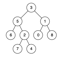
Input: root = [3,5,1,6,2,0,8,null,null,7,4], p = 5, q = 1 Output: 3 Explanation: The LCA of nodes 5 and 1 is 3.
Example 2:
Input: root = [3,5,1,6,2,0,8,null,null,7,4], p = 5, q = 4 Output: 5 Explanation: The LCA of nodes 5 and 4 is 5, since a node can be a descendant of itself according to the LCA definition.
Example 3:
Input: root = [1,2], p = 1, q = 2 Output: 1
Constraints:
- The number of nodes in the tree is in the range
[2, 10=^{=5}=]=. -10=^{=9}= <= Node.val <= 10=9- All
Node.valare unique. p !q=pandqwill exist in the tree.
※ 2.8.17.1. Constraints and Edge Cases
<list constraints, input limits, or tricky edge cases here>
※ 2.8.17.2. My Solution (Code)
※ 2.8.17.2.1. v1: fast, recursive checks:
1: # Definition for a binary tree node. 2: # class TreeNode: 3: # def __init__(self, x): 4: # self.val = x 5: # self.left = None 6: # self.right = None 7: 8: class Solution: 9: │ def lowestCommonAncestor(self, root: 'TreeNode', p: 'TreeNode', q: 'TreeNode') -> 'TreeNode': 10: │ │ # Base case: if root is None or root matches p or q 11: │ │ if not root or root == p or root == q: 12: │ │ │ return root 13: │ │ │ 14: │ │ # Recur for left and right subtrees 15: │ │ left = self.lowestCommonAncestor(root.left, p, q) 16: │ │ right = self.lowestCommonAncestor(root.right, p, q) 17: │ │ 18: │ │ # If both left and right are non-null, this is the LCA 19: │ │ if left and right: 20: │ │ │ return root 21: │ │ │ 22: │ │ # Otherwise return the non-null child (either left or right) 23: │ │ return left if left else right
※ 2.8.17.2.2. v2: slow, iterative DFS with root comparisons
1: from collections import deque 2: 3: class Solution: 4: │ def lowestCommonAncestor(self, root: 'TreeNode', p: 'TreeNode', q: 'TreeNode') -> 'TreeNode': 5: │ │ if not root or root == p or root == q: 6: │ │ │ return root 7: │ │ │ 8: │ │ # i want to compare paths, I will get the paths by doing tree-walks 9: │ │ stack = [(root, [])] 10: │ │ p_path, q_path = None, None 11: │ │ 12: │ │ while stack: 13: │ │ │ node, parent_path = stack.pop() 14: │ │ │ curr_path = parent_path + [node] 15: │ │ │ 16: │ │ │ if node == p: 17: │ │ │ │ p_path = curr_path 18: │ │ │ if node == q: 19: │ │ │ │ q_path = curr_path 20: │ │ │ │ 21: │ │ │ if p_path and q_path: 22: │ │ │ │ break 23: │ │ │ │ 24: │ │ │ if node.left: 25: │ │ │ │ stack.append((node.left, curr_path + [node])) 26: │ │ │ if node.right: 27: │ │ │ │ stack.append((node.right, curr_path + [node])) 28: │ │ │ │ 29: │ │ ans = root 30: │ │ for p_node, q_node in zip(p_path, q_path): 31: │ │ │ if p_node != q_node: 32: │ │ │ │ return ans 33: │ │ │ ans = p_node 34: │ │ │ 35: │ │ return ans
※ 2.8.17.2.3. v3: optimised iterative DFS with parent tracking
1: # Definition for a binary tree node. 2: # class TreeNode: 3: # def __init__(self, x): 4: # self.val = x 5: # self.left = None 6: # self.right = None 7: 8: class Solution: 9: │ def lowestCommonAncestor(self, root: 'TreeNode', p: 'TreeNode', q: 'TreeNode') -> 'TreeNode': 10: │ │ # trivial early returns 11: │ │ if not root: 12: │ │ │ return None 13: │ │ │ 14: │ │ stack = [(root, None)] # node, parent 15: │ │ node_to_parent = {root: None} # maps node to parent 16: │ │ 17: │ │ # find both p and q: 18: │ │ while p not in node_to_parent or q not in node_to_parent: 19: │ │ │ node, parent = stack.pop() 20: │ │ │ node_to_parent[node] = parent 21: │ │ │ if node.left: 22: │ │ │ │ stack.append((node.left, node)) 23: │ │ │ │ 24: │ │ │ if node.right: 25: │ │ │ │ stack.append((node.right, node)) 26: │ │ │ │ 27: │ │ # now with preprocessed info, we get ancestors: 28: │ │ ancestors = set() 29: │ │ while p: 30: │ │ │ ancestors.add(p) 31: │ │ │ p = node_to_parent[p] 32: │ │ │ 33: │ │ # now traverse q, comparatively 34: │ │ while q not in ancestors: 35: │ │ │ q = node_to_parent[q] 36: │ │ │ 37: │ │ return q
※ 2.8.17.3. My Approach/Explanation
NOt sure how to make the iterative version faster.
※ 2.8.17.4. My Learnings/Questions
<what did you learn? any uncertainties or questions?>
※ 2.8.17.5. [Optional] Additional Context
<e.g., “I struggled with X”, “I want to know about alternative algorithms”, etc.>
※ 2.9. Tries
| Headline | Time | ||
|---|---|---|---|
| Total time | 2:21 | ||
| Tries | 2:21 | ||
| [60] Implement Trie (Prefix Tree) (208) | 0:36 | ||
| [61] Design Add and Search Words Data… | 1:14 | ||
| ⭐️ [62] Word Search II (212) | 0:31 |
※ 2.9.1. General Notes
※ 2.9.1.1. Fundamentals
- root-to-leaf paths represents strings
- nodes may have any number of children
- We need to have terminus encoded
approach 1: terminal nodes
need to be able to distinguish string ends from prefixes. So string ends should have some way to determine that it’s the end (e.g. some delimiter that should be added as a leaf)
- approach 2: use special flag in the node
- compression:
- if the char space is known, we can just use fixed length lists and do edit distance based indexing
- Trie Applications
- String dictionaries
- Searching
- Sorting / enumerating strings
- Partial string operations:
- Prefix queries: find all the strings that start with pi.
- Long prefix: what is the longest prefix of “pickling” in the trie?
- Wildcards: find a string of the form “pi??le” in the trie.
- String dictionaries
※ 2.9.1.1.1. Misconceptions
This is the misconception:
“Each Trie node stores a character (val), and during traversal, we should compare node.val = char=.”
- The Trie is composed of edges labeled with characters, not nodes tied to characters.
- The parent points to children via keys such as
node.children['a']. - The child node doesn’t need to know which character got you there — the parent’s edge label is sufficient.
The correct operation is:
Show/Hide Python Codeif char in node.children: │ node = node.children[char]
Incorrect operation:
Show/Hide Python Code1: if node.val == char: 2: │ # This confuses node identity with edge traversal
Nodes do not decide what they are — parents decide how you reach them. All traversal decisions are based on the key in the .children dictionary, not on the node’s own value.
Summary:
| Concept | Clarification |
|---|---|
| Trie Node stores character | False; character is associated with the edge, not the node |
| `node.val == char` traversal | Incorrect: you’re matching the wrong layer of abstraction |
| Proper traversal strategy | Use `node.children[char]` to find valid transitions |
| Role of `val` | Optional; useful only for debugging or visualization |
| Trie view | The character path is encoded in the edges, not in the node values |
※ 2.9.2. [60] Implement Trie (Prefix Tree) (208)
A trie (pronounced as “try”) or prefix tree is a tree data structure used to efficiently store and retrieve keys in a dataset of strings. There are various applications of this data structure, such as autocomplete and spellchecker.
Implement the Trie class:
Trie()Initializes the trie object.void insert(String word)Inserts the stringwordinto the trie.boolean search(String word)Returnstrueif the stringwordis in the trie (i.e., was inserted before), andfalseotherwise.boolean startsWith(String prefix)Returnstrueif there is a previously inserted stringwordthat has the prefixprefix, andfalseotherwise.
Example 1:
Input
["Trie", "insert", "search", "search", "startsWith", "insert", "search"]
[[], ["apple"], ["apple"], ["app"], ["app"], ["app"], ["app"]]
Output
[null, null, true, false, true, null, true]
Explanation
Trie trie = new Trie();
trie.insert("apple");
trie.search("apple"); // return True
trie.search("app"); // return False
trie.startsWith("app"); // return True
trie.insert("app");
trie.search("app"); // return True
Constraints:
1 <word.length, prefix.length <= 2000=wordandprefixconsist only of lowercase English letters.- At most
3 * 10=^{=4} calls in total will be made toinsert,search, andstartsWith.
※ 2.9.2.1. Constraints and Edge Cases
Nothing fancy, just the meaning of “startsWith” is important.
- You also correctly handle all edge cases:
- Words that are prefixes of others (apple, app),
- Searching for a prefix that was not inserted,
- Checking
startsWith()independently of the terminal flag.
※ 2.9.2.2. My Solution (Code)
1: class Node: 2: │ def __init__(self, val=None, terminal=False): 3: │ │ self.val = val 4: │ │ self.children = dict() # character_to_child map 5: │ │ self.terminal = terminal 6: │ │ 7: │ │ 8: class Trie: 9: │ def __init__(self): 10: │ │ self.root = Node() # will be empty first 11: │ │ 12: │ def insert(self, word: str) -> None: 13: │ │ ptr = self.root 14: │ │ for char in word: 15: │ │ │ if not char in ptr.children: 16: │ │ │ │ ptr.children[char] = Node(val=char) 17: │ │ │ │ 18: │ │ │ ptr = ptr.children[char] 19: │ │ │ 20: │ │ # ptr is at terminal char: 21: │ │ ptr.terminal = True 22: │ │ 23: │ │ 24: │ def search(self, word: str) -> bool: 25: │ │ ptr = self.root 26: │ │ for char in word: 27: │ │ │ if char not in ptr.children: 28: │ │ │ │ return False 29: │ │ │ else: 30: │ │ │ │ ptr = ptr.children[char] 31: │ │ │ │ 32: │ │ # has to have terminal flag set 33: │ │ return ptr.terminal 34: │ │ 35: │ │ 36: │ def startsWith(self, prefix: str) -> bool: 37: │ │ ptr = self.root 38: │ │ for char in prefix: 39: │ │ │ if char not in ptr.children: 40: │ │ │ │ return False 41: │ │ │ else: 42: │ │ │ │ ptr = ptr.children[char] 43: │ │ │ │ 44: │ │ │ │ 45: │ │ return True 46: │ │ # return not ptr.terminal 47: │ │ 48: │ │ 49: │ │ 50: # Your Trie object will be instantiated and called as such: 51: # obj = Trie() 52: # obj.insert(word) 53: # param_2 = obj.search(word) 54: # param_3 = obj.startsWith(prefix)
Complexity Analysis
Assuming:
\(n\) = length of word/prefix,
\(k\) = total number of insert/search/startsWith calls,
\(\sum\) = number of possible characters (here \(\sum\) = 26 lowercase letters):
Time Complexity:
insert: \(O(n)\)
search: \(O(n)\)
startsWith: \(O(n)\)
A cleaner solution to this (minor improvements):
1: class TrieNode: 2: │ def __init__(self): 3: │ │ self.children = {} 4: │ │ self.terminal = False 5: │ │ 6: class Trie: 7: │ def __init__(self): 8: │ │ self.root = TrieNode() 9: │ │ 10: │ def insert(self, word): 11: │ │ node = self.root 12: │ │ for ch in word: 13: │ │ │ if ch not in node.children: 14: │ │ │ │ node.children[ch] = TrieNode() 15: │ │ │ node = node.children[ch] 16: │ │ node.terminal = True 17: │ │ 18: │ def search(self, word): 19: │ │ node = self._traverse(word) 20: │ │ return node is not None and node.terminal 21: │ │ 22: │ def startsWith(self, prefix): 23: │ │ return self._traverse(prefix) is not None 24: │ │ 25: │ def _traverse(self, string): 26: │ │ node = self.root 27: │ │ for ch in string: 28: │ │ │ if ch not in node.children: 29: │ │ │ │ return None 30: │ │ │ node = node.children[ch] 31: │ │ return node 32:
※ 2.9.2.2.1. Possible Improvements
The only alternative that could be faster (in constant time) is replacing dict with a fixed-size array for children (at the cost of more space). But that is a trade-off — and your choice is more Pythonic for readability and generality.
※ 2.9.2.3. My Approach/Explanation
For trie, I’ll add in my own implementation for Node in the trie.
For terminal, I’ll place it as a flag within the node, that should be easy.
※ 2.9.2.4. My Learnings/Questions
- Pythonic Improvements
- Use
collections.defaultdict(Node)for auto-adding children (optional). node.children.get(ch)can be used instead ofif ch not in ...in some cases.- Remove
valfromNodeunless used for debugging.
- Use
- I think my approach of having a dummy node as the root works well here.
I didn’t understand the requirements for the
startsWithfunction. I was too strict about it (that it can’t be a terminus, so that’s the bug I had)What
startsWithShould Do:It should return
Trueif any word in the trie starts with the given prefix, regardless of whether the prefix is a complete word by itself (i.e.,terminal=True) or not.
※ 2.9.2.5. [Optional] Additional Context
Pretty happy with this, I implemented it correctly.
※ 2.9.3. [61] Design Add and Search Words Data Structure (211)
Design a data structure that supports adding new words and finding if a string matches any previously added string.
Implement the WordDictionary class:
WordDictionary()Initializes the object.void addWord(word)Addswordto the data structure, it can be matched later.bool search(word)Returnstrueif there is any string in the data structure that matcheswordorfalseotherwise.wordmay contain dots'.'where dots can be matched with any letter.
Example:
Input
["WordDictionary","addWord","addWord","addWord","search","search","search","search"]
[[],["bad"],["dad"],["mad"],["pad"],["bad"],[".ad"],["b.."]]
Output
[null,null,null,null,false,true,true,true]
Explanation
WordDictionary wordDictionary = new WordDictionary();
wordDictionary.addWord("bad");
wordDictionary.addWord("dad");
wordDictionary.addWord("mad");
wordDictionary.search("pad"); // return False
wordDictionary.search("bad"); // return True
wordDictionary.search(".ad"); // return True
wordDictionary.search("b.."); // return True
Constraints:
1 <word.length <= 25=wordinaddWordconsists of lowercase English letters.wordinsearchconsist of'.'or lowercase English letters.- There will be at most
2dots inwordforsearchqueries. - At most
10=^{=4} calls will be made toaddWordandsearch.
※ 2.9.3.1. Constraints and Edge Cases
All valid cases in the problem are supported, including:
search(“b..”) → matches multiple nodes,
search(“.ad”) → wildcard at front,
search(“pad”) → no match
※ 2.9.3.2. My Solution (Code)
1: class Node: 2: │ def __init__(self, val=None, terminal=False): 3: │ │ self.children = dict() 4: │ │ self.val = val 5: │ │ self.terminal = terminal 6: │ │ 7: class WordDictionary: 8: │ def __init__(self): 9: │ │ self.root = Node() 10: │ │ self.wild = "." 11: │ │ 12: │ def addWord(self, word: str) -> None: 13: │ │ ptr = self.root 14: │ │ for char in word: 15: │ │ │ if char not in ptr.children: 16: │ │ │ │ ptr.children[char] = Node(val=char) 17: │ │ │ ptr = ptr.children[char] 18: │ │ # terminate: 19: │ │ ptr.terminal = True 20: │ │ 21: │ │ return
it’s the search function that I didn’t implement right the first time round.
A wildcard just means that we should consider ALL the children for our BFS/DFS.
Here’s the corrected version for the search function
1: def search(self, word: str) -> bool: 2: │ options = [self.root] 3: │ 4: │ for idx, char in enumerate(word): 5: │ │ next_options = [] 6: │ │ 7: │ │ for node in options: 8: │ │ │ if char == self.wild: 9: │ │ │ │ # Try all possible children 10: │ │ │ │ next_options.extend(node.children.values()) 11: │ │ │ else: 12: │ │ │ │ if char in node.children: 13: │ │ │ │ │ next_options.append(node.children[char]) 14: │ │ │ │ │ 15: │ │ # No valid paths 16: │ │ if not next_options: 17: │ │ │ return False 18: │ │ │ 19: │ │ options = next_options 20: │ │ 21: │ # After processing all characters, check terminal flag 22: │ return any(node.terminal for node in options)
The buggy version for the search is below, see the reasons why they were buggy:
- Complexity Analysis
- Assume:
- \(n\) = length of search word
- \(m\) = total number of words added
- \(\sum\) = 26 (lowercase English letters)
addWord:- Time: \(O(n)\) per word
- Space: \(O(n)\) new nodes in worst case (word is new)
- search (worst case: wildcards):
- Time: \(O(\sum^{2} * n)\)
- With 2 wildcards in the word (max allowed), it can try all combinations among children.
- In practice, this is fast due to short word lengths (≤25) and limited total calls (≤10⁴).
- Space: \(O(n)\) recursion depth or BFS queue depth
- Time: \(O(\sum^{2} * n)\)
- Assume:
※ 2.9.3.2.1. Alternative DFS version
This might feel a little more natural
1: class WordDictionary: 2: │ def __init__(self): 3: │ │ self.root = dict() 4: │ │ self.terminal = "#" 5: │ │ 6: │ def addWord(self, word): 7: │ │ node = self.root 8: │ │ for ch in word: 9: │ │ │ node = node.setdefault(ch, {}) 10: │ │ node[self.terminal] = True 11: │ │ 12: │ def search(self, word): 13: │ │ def dfs(i, node): 14: │ │ │ if i == len(word): 15: │ │ │ │ return self.terminal in node 16: │ │ │ ch = word[i] 17: │ │ │ if ch == ".": 18: │ │ │ │ return any(dfs(i + 1, next_node) for next_node in node.values() if isinstance(next_node, dict)) 19: │ │ │ if ch not in node: 20: │ │ │ │ return False 21: │ │ │ return dfs(i + 1, node[ch]) 22: │ │ │ 23: │ │ return dfs(0, self.root) 24:
※ 2.9.3.2.2. Buggy Attempt at a BFS solution for the search() function
1: │ def search(self, word: str) -> bool: 2: │ │ # options nodes to try out: 3: │ │ options = [self.root] 4: │ │ for idx, char in enumerate(word): 5: │ │ │ if not options: 6: │ │ │ │ return False 7: │ │ │ # need to ignore this level and move on 8: │ │ │ if char == self.wild: 9: │ │ │ │ # true by default: 10: │ │ │ │ if idx == len(word) - 1: 11: │ │ │ │ │ return True 12: │ │ │ │ │ 13: │ │ │ │ # add all children as options 14: │ │ │ │ options = (child_ptr for option in options for child_ptr in option.children) 15: │ │ │ │ continue 16: │ │ │ else: 17: │ │ │ │ 18: │ │ │ │ if idx == len(word) - 1: 19: │ │ │ │ │ return any([option for option in options if option.val == char and option.terminal]) 20: │ │ │ │ valid_options = [option for option in options if option.val == char] 21: │ │ │ │ # QQ: does this ensure the generator can generate one value at least? 22: │ │ │ │ if not valid_options: 23: │ │ │ │ │ return False 24: │ │ │ │ options = valid_options 25: │ │ │ │ 26: │ │ return False
Problems:
❌ Misuse of .val comparison instead of structured traversal
When this is written,
valid_options = [option for option in options if option.val =char]=You are comparing
char =option.val=, but that’s not how a Trie works.The Trie works by following edges (child pointers) labeled with characters, not by checking the character stored in the node.
The character stored in a node (val) is only for debugging or tracking — it shouldn’t be used for traversal.
when processing
charwe need to actually move to that valid option so instead of just picking that optionso instead of
char in option.children, move tooption.children[char]You are returning
Truejust because you saw a"."at the last index. This is incorrect — the wildcard must still match any child node that is also terminal, not just exist!Fix: You need to explore all possible paths for “.”, especially at the last character.
You need to look ahead one level, and if any of the children match the rest of the string, return True.
※ 2.9.3.3. My Approach/Explanation
- similar trie implementation
- for the wildcard searching we need to be able to add the whole layer as search options.
※ 2.9.3.4. My Learnings/Questions
- We can remove the
valattribute from the trie node. - Completely different approaches:
Regex matching
we could use regexes, but it would be to slow (would work though). Downside: \(O(mn)\) complexity with linear scan per search, and regex compilation overhead.
Show/Hide Python Code1: import re 2: 3: class WordDictionary: 4: │ def __init__(self): 5: │ │ self.words = [] 6: │ │ 7: │ def addWord(self, word): 8: │ │ self.words.append(word) 9: │ │ 10: │ def search(self, word): 11: │ │ pattern = re.compile(f"^{word}$") 12: │ │ return any(pattern.match(w) for w in self.words)
- Ternary Search Tree (TST) More memory-efficient than a full Trie in certain contexts. TSTs are node-based but maintain 3 branches per node (less than, equal, greater). This is only useful when space savings are substantial and rarely benefits wildcard matching directly.
My mental model for tries was a little inferior.
TLDR;
This is a misconception: “Each node in the Trie represents a character, so to find a word, I should walk the tree comparing the node’s .val field to characters in the word.”
A trie should just be seen as a map of maps.
Each path from the root to a node represents a prefix (or whole) of a word.
The Node itself is not what stores the “current character”.
The edge from a parent to that node is labelled with a character from the word.
The node pointed to by ’c’ edge doesn’t need to know what its character is — its parent does.
That’s why we can avoid the val attribute from the custom helper Node class that we write
Show/Hide Python Code1: class Node: 2: │ def __init__(self): 3: │ │ self.children = dict() 4: │ │ self.terminal = False 5:
Read more details about this misconception here:
Show/Hide Md CodeYou're asking a **great** question! Let's clarify this fully — conceptually and practically — and help you **internalize how a Trie works**, especially the part about edge labels (characters) versus node values (`val`). ## 🧠 The Misconception vs. The Reality ### ❌ **Misconception:** > "Each node in the Trie **represents** a character, so to find a word, I should walk the tree comparing the node’s `.val` field to characters in the word." This is intuitive at first glance — after all, you stored the character in `Node.val`, right? But **that’s not how a Trie actually functions**. ## ✅ **Correct Mental Model: The Trie as a Map of Maps** Let’s break it down clearly: ### 1. **The Trie is a tree of **paths**, not labels** Each path from the root to a node represents a **prefix (or whole)** of a word. - The `Node` itself is **not** what stores the "current character". - The **edge from a parent to that node** is labeled with a character from the word. 🧭 So when inserting "cat": ``` │ │ root │ │ │| │ │ 'c' │ │ │| │ │ 'a' │ │ │| │ │ 't' ← terminal node (word ends here) ``` - The node pointed to by `'c'` edge doesn’t *need* to know what its character is — its parent does. - Edge: `"c"` → Node │ Edge: `"a"` → Node │ Edge: `"t"` → Node (terminal) │ ✔️ We use `.children[char]` to **ask the current node: "Do you have a child along the edge labeled `'c'`?"** ### 2. **Node.val is *not required for functionality*** You **can build** a correct and fully functional Trie without storing any character in the Node: ```python class Node: │ def __init__(self): │ │ self.children = dict() │ │ self.terminal = False ``` You **don’t need** the node to know what character it "represents" because traversal **is guided by keys in the `.children` dictionary**. You say: ```python if char in node.children: │ node = node.children[char] ``` You're **not checking `node.val == char`** because: - You already told the trie which character you're looking for (the dictionary key). - That **edge** — the mapping in `children` — **is** the character. ## 🧠 Analogy: Directory Structure Think of a Trie like a file system: ```plaintext / ├── u │ └── s │ └── e │ └── r │ └── s │ └── .txt ``` You don’t ask each folder: > "Are you named 'u'?" → "Are you named 's'?" → etc. Instead, you follow the **map** of nested directories: ```python if "u" in root: │ root = root["u"] ``` The **key** at each level defines the "label"; you don't ask the value if it equals something. ## ✅ Why Comparing `node.val == char` is Wrong (in search) Because: 1. You're analyzing the current node, *not* its parent’s children map. 2. You don’t know *what edge* got you here. 3. You should decide “where to go from here,” not “what am I.” ```python if char in node.children: # ✅ correct │ node = node.children[char] │ if node.val == char: # ❌ incorrect │ do something... ``` Again, `node.val` exists purely (maybe) to help print/debug the trie — not for path logic. ## ✅ Internalize This Mental Model: ``` A Trie node has: - Edges (char → child) - A Boolean: is_terminal To find a word: - Start at the root. - For each character in the word: │ - Follow the child at .children[char] ``` So you always think: > "What **option** can I pick **next**, labeled by this character?" ## ✅ Optional: Visualization (Bonus) Let me serialize a trie with words: `["apple", "app", "bat"]` ``` root ├── 'a' │ └── 'p' │ └── 'p' (*) │ └── 'l' │ └── 'e' (*) ├── 'b' │ └── 'a' │ │ └── 't' (*) ``` Where `(*)` means terminal node — a full word ends here. Notice how every node is connected via labeled edges — *"use this character to walk the tree and find possible completions."* ## ✅ TL;DR Summary | Concept | Explanation | |--------|-------------| | ⭐ Trie's children map (`.children`) | Maps characters (edges) to child nodes | | 🚫 `node.val` is not traversal logic | It's metadata — the path is in `.children` | | ✅ To check next character | Use `if char in node.children`, not `node.val == char` | | ❌ Traversing by matching `.val` | Fails when multiple child nodes are present | Let me know if you'd like: - ⚙️ an animation/step-by-step of word search - 🗺️ a trie visual in dot/graphviz - 📦 help stripping `val` entirely for cleaner trie's performance Happy to help clarify until it clicks!
※ 2.9.4. ⭐️⭐️[62] Word Search II (212) redo hard tedious
Given an m x n board of characters and a list of strings words,
return all words on the board.
Each word must be constructed from letters of sequentially adjacent cells, where adjacent cells are horizontally or vertically neighboring. The same letter cell may not be used more than once in a word.
Example 1:
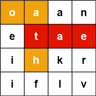
Input: board = [["o","a","a","n"],["e","t","a","e"],["i","h","k","r"],["i","f","l","v"]], words = ["oath","pea","eat","rain"] Output: ["eat","oath"]
Example 2:
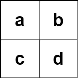
Input: board = [["a","b"],["c","d"]], words = ["abcb"] Output: []
Constraints:
m =board.length=n =board[i].length=1 <m, n <= 12=board[i][j]is a lowercase English letter.1 <words.length <= 3 * 10=41 <words[i].length <= 10=words[i]consists of lowercase English letters.- All the strings of
wordsare unique.
※ 2.9.4.1. Constraints and Edge Cases
- pruning should always be considered.
※ 2.9.4.2. My Solution (Code)
※ 2.9.4.2.1. Optimal Solution
I’m just putting this in first, I’ll come back to this question another time.
This solution is pretty genious, I love how pretty it is.
1: from typing import List 2: 3: class TrieNode: 4: │ def __init__(self): 5: │ │ self.children = {} 6: │ │ self.word = None # store word at the end node for easy result collection 7: │ │ 8: class Solution: 9: │ def findWords(self, board: List[List[str]], words: List[str]) -> List[str]: 10: │ │ # Step 1: Build Trie from words 11: │ │ root = TrieNode() 12: │ │ for word in words: 13: │ │ │ node = root 14: │ │ │ for char in word: 15: │ │ │ │ node = node.children.setdefault(char, TrieNode()) 16: │ │ │ node.word = word # mark the end of a word 17: │ │ │ 18: │ │ rows, cols = len(board), len(board[0]) 19: │ │ result = [] 20: │ │ 21: │ │ # Step 2: Backtracking DFS with Trie pruning 22: │ │ def dfs(r, c, node): 23: │ │ │ char = board[r][c] 24: │ │ │ curr = node.children.get(char) 25: │ │ │ if not curr: 26: │ │ │ │ return 27: │ │ │ │ 28: │ │ │ if curr.word: 29: │ │ │ │ result.append(curr.word) 30: │ │ │ │ curr.word = None # prevent duplicates 31: │ │ │ │ 32: │ │ │ board[r][c] = '#' # mark as visited 33: │ │ │ 34: │ │ │ for dr, dc in [(-1,0),(1,0),(0,-1),(0,1)]: # up, down, left, right 35: │ │ │ │ nr, nc = r + dr, c + dc 36: │ │ │ │ if 0 <= nr < rows and 0 <= nc < cols and board[nr][nc] != '#': 37: │ │ │ │ │ dfs(nr, nc, curr) 38: │ │ │ │ │ 39: │ │ │ board[r][c] = char # restore 40: │ │ │ 41: │ │ │ # Optional: prune leaf nodes in Trie to optimize further 42: │ │ │ if not curr.children: 43: │ │ │ │ node.children.pop(char) 44: │ │ │ │ 45: │ │ # Step 3: Start DFS from each cell 46: │ │ for r in range(rows): 47: │ │ │ for c in range(cols): 48: │ │ │ │ dfs(r, c, root) 49: │ │ │ │ 50: │ │ return result 51:
※ 2.9.4.2.2. Retro solution on Depth D2
1: from collections import defaultdict 2: 3: class Node: 4: │ def __init__(self): 5: │ │ self.children = defaultdict(Node) 6: │ │ self.word = None 7: │ │ 8: class Solution: 9: │ def findWords(self, board: List[List[str]], words: List[str]) -> List[str]: 10: │ │ ROWS, COLS = len(board), len(board[0]) 11: │ │ DIRS = [(1, 0), (-1, 0), (0, 1), (0, -1)] 12: │ │ VISITED = "*" 13: │ │ 14: │ │ res = [] 15: │ │ 16: │ │ # we build the trie: 17: │ │ root = Node() 18: │ │ for w in words: 19: │ │ │ ptr = root 20: │ │ │ for c in w: 21: │ │ │ │ ptr = ptr.children[c] 22: │ │ │ ptr.word = w 23: │ │ │ 24: │ │ def backtrack(r, c, node): 25: │ │ │ cell = board[r][c] 26: │ │ │ 27: │ │ │ if cell not in node.children: 28: │ │ │ │ return 29: │ │ │ │ 30: │ │ │ child = node.children[cell] 31: │ │ │ if child.word: 32: │ │ │ │ res.append(child.word) 33: │ │ │ │ child.word = None # set it off 34: │ │ │ │ 35: │ │ │ │ # OPTIMISATION: remove if the child has no children: 36: │ │ │ │ if not child.children: 37: │ │ │ │ │ node.children.pop(cell) 38: │ │ │ │ │ 39: │ │ │ board[r][c] = VISITED 40: │ │ │ 41: │ │ │ for row, col in ((r + dr, c + dc) for dr, dc in DIRS if ( 42: │ │ │ │ 0 <= r + dr < ROWS and 0 <= c + dc < COLS and board[r + dr][c + dc] != VISITED 43: │ │ │ │ )): 44: │ │ │ │ # choose it: 45: │ │ │ │ backtrack(row, col, child) 46: │ │ │ │ 47: │ │ │ board[r][c] = cell 48: │ │ │ 49: │ │ │ return 50: │ │ │ 51: │ │ for row, col in ((r, c) for r in range(ROWS) for c in range(COLS)): 52: │ │ │ backtrack(row, col, root) 53: │ │ │ 54: │ │ return res
※ 2.9.4.3. My Approach/Explanation
This is guided a bit.
I know that we need to do DFSes to check the for words in the board.
Let’s consider the brute force approach then.
- For each word, check every cell as a potential start and do a DFS for every word from every cell
- Downside: Extremely inefficient for large boards and word lists, because you repeat the same searches for common prefixes over and over.
This reveals the main trick: to reduce the input space we get if we convert the entry list into a trie. Then we don’t need to waste resources having to re-evaluate the prefixes that we’ve already found.
A Trie helps you batch together searches that start with the same letters, efficiently pruning dead ends
- Step-by-step:
- Build a Trie for all words
- Before any board search, put all words into a Trie.
- Each Trie node represents a possible prefix, and marks the end of a word
- Start Backtracking DFS from every cell on the board
- For each cell,
- If its character matches a starting character in the Trie, try to go deeper in the trie (recursively search neighbors for the next character in a matching Trie branch)
- For each cell,
- Only explore further if your prefix is still valid
- At every cell, move to its neighbors (up, down, left, right)
- Each time, check if your path so far is still a prefix in the Trie.
- If at any point the path is not in the Trie, stop—no word can possibly start with this path.
- If you reach a Trie node that marks a word’s end, record the word
- Avoid duplicates by marking the Trie node as “used” or deleting the word after you find it once
- Build a Trie for all words
- So the pseudocode is this:
1: for each word in words: 2: insert into trie 3: 4: for i in range(rows): 5: for j in range(cols): 6: │ │ dfs(board, i, j, trie_root)
- Backtracking:
- Temporarily mark the visited cell (e.g., set to ’#’) to avoid revisiting.
- After recursive calls, restore the original letter.
※ 2.9.4.4. My Learnings/Questions
- entertain the brute force approach to identify where the wasted processing is at and how to improve on that. The trick here would have been possible to get if we tried to prune the duplication.
- Rough implementation sketch:
- Build one Trie for all words.
- For each board cell, try to explore words starting there using the Trie.
- DFS and backtracking through the board, checking Trie as you go.
- Prune dead branches early using Trie.
For this particular question, some things to note:
- it’s important to explore the brute force solution asap. This will highlight the source of friction in the brute force, which is what we need to solve. That’s how we can do the step-by-step socratic approach.
- so if we know that we want to avoid multiple prefix-searches \(\implies\) we want to keep all the target words as a trie to avoid duplicate searching efforts.
- we know that it’s going to be DFS-like.
In the dfs() function, you’re walking the Trie and the board simultaneously
How can the trie help us with this? For each cell, try to use it as the starting point for the trie and exploit the depth around it. This gives some improvements / augmentations that make life easy:
- if we keep the entire word at the node as the terminus, then it’s easy for us to directly return it
- to “store visited” we just need to temporarily set the current node as visited (since it’s going to be a pre-order DFS traversal that we will be conducting). We can restore it after we check all possibilities and the thing returns.
- we can prune!
for more context on how/why the pruning works:
Show/Hide Md Code│ Great question! The line: │ │ ```python │ if not curr.children: │ node.children.pop(char) │ ``` │ │ is an **optimization step** that **prunes (removes) leaf nodes** in the Trie as they become unnecessary during the search. Let's break it down: │ │ ## 📌 Context │ │ In the `dfs()` function, you're walking the Trie and the board simultaneously. │ │ When you **find a word**, you mark `curr.word = None` to avoid finding it again (de-duplication). │ │ But what if the part of the Trie you just used is no longer useful? │ │ That's where this line comes in: │ │ ```python │ if not curr.children: │ node.children.pop(char) │ ``` │ │ ## 🧠 What It Actually Does │ │ - `curr` is the Trie node for the current letter (`char`). │ - After the recursive DFS call for all directions: │ - If `curr.children` is empty, that means no words remain that depend on this node. │ - So we `pop(char)` from the parent (`node.children`) to remove the branch entirely. │ │ ➡️ This helps reduce the size of the Trie **during the search itself**, so that: │ - Future DFS searches do **fewer lookups** │ - You **avoid redundant work** looking up dead branches │ │ ## ✅ Why Is This Safe? │ │ Because each node in the Trie corresponds to a **prefix**. │ So: │ │ - If a node has `children`, other words still depend on it → 🔒 keep it │ - If a node: │ - Has no children (`curr.children == {}`) │ - Has no word (`curr.word == None`) │ then ➡️ it’s a **dead end** and can be safely removed │ │ ### 🔄 Example: │ │ Say your word list was: │ │ ```python │ ["apple", "app"] │ ``` │ │ Your Trie branches would look like: │ │ ``` │ a │ └── p │ └── p (* "app") │ │ │ └── l │ │ │ └── e (* "apple") │ ``` │ │ When you find `"apple"`: │ - You set `word = None` on node `'e'` │ - Now node `'e'` has no `children` and no word. │ - So you delete `'e'` from its parent `'l'`. │ │ Same for `'l'`, and `'p'`, once `"app"` is found. │ │ Eventually, this whole `"apple"` branch gets pruned as unused, saving space and lookup time. │ │ ## 🚀 Summary Table │ │ | Condition | What it means | What we do | │ |-----------------------------|----------------------------|-------------------------| │ | `not curr.children` | No more words from here | Safe to prune this node | │ | `curr.word = None` | Word already found | No need to revisit | │ | `node.children.pop(char)` | Delete from parent node | Clean up the Trie | │ │ ## 🧠 Big Picture │ │ Trie pruning is like smart garbage collection: │ If we **used a branch**, and it's no longer useful, we cut it off ✂️ to avoid future wasted search time. │ │ ### ⚠️ Note: │ This is an **optimization**, not required for correctness — │ but it gives a noticeable **performance boost** on large inputs with many overlapping prefixes. │ │ Let me know if you want to **visualize this pruning process step by step**, or simulate it on an example like `["cat", "car", "cart"]` — I'd be happy to walk you through it!
※ 2.9.4.5. [Optional] Additional Context
Honestly this was a little tough. I hope just exposure for this makes me able to solve similar things.
Even in the retro, the accuracy required to get this right feels a little high right now. IT requires calmness and clarity of thought to be able to avoid silly accuracy bugs.
※ 2.9.4.6. Retros
※ 2.9.4.6.1.
I redid this, but was just slightly off. The trie building had some initial friction, but I got it right.
Here’s my TrieNode:
1: class TrieNode(): 2: │ def __init__(self): 3: │ │ self.children = defaultdict(TrieNode) 4: │ │ self.word = word # we can early get from this instead of needing to walk from the root to this node again. 5: │ │ 6: # built using: # we build the trie: 7: │ │ root = Node() 8: │ │ for w in words: 9: │ │ │ ptr = root 10: │ │ │ for c in w: 11: │ │ │ │ ptr = ptr.children[c] 12: │ │ │ ptr.word = w
I made a few accuracy mistakes like so:
- not returning state after committing a choice
- not turning the word off after finding the word (thereby leading to duplicate finds)
Additionally, I didn’t think of the trie-pruning option either. The idea here is that when we find a word, other than just “turning it off” so that we don’t double count, we can check if there are no children in that word. If so, we can just remove that char from its parent:
1: │ │ cell = board[r][c] 2: │ │ │ if cell not in node.children: 3: │ │ │ │ return 4: │ │ │ │ 5: │ │ │ child = node.children[cell] 6: │ │ │ if child.word: 7: │ │ │ │ res.append(child.word) 8: │ │ │ │ child.word = None # set it off to prevent double counting 9: │ │ │ │ 10: │ │ │ │ # OPTIMISATION: remove if the child has no children: 11: │ │ │ │ if not child.children: 12: │ │ │ │ │ node.children.pop(cell)
※ 2.10. Backtracking
| Headline | Time | |||
|---|---|---|---|---|
| Total time | 20:27 | |||
| Backtracking | 20:27 | |||
| [63] Subsets (78) | 13:32 | |||
| My Solution (Code) | 12:54 | |||
| [64] Combination Sum (39) | 0:54 | |||
| [65] Combination Sum II (40) | 2:37 | |||
| [67] Permutations (46) | 0:18 | |||
| [68] Subsets II (90) | 0:23 | |||
| [69] Word Search (79) | 0:29 | |||
| [70] Palindrome Partitioning (131) | 0:36 | |||
| [71] Letter Combinations of a Phone… | 0:23 | |||
| [72] N-Queens (51) | 1:15 |
※ 2.10.1. General Notes
※ 2.10.1.1. Fundamentals
Framework: Recursion + state tracing + pruning/subtree skipping (if a constraint is violated).
Pattern: Make a choice → Recurse → Undo choice.
Common Use Cases: Generating combinations, permutations, subset enumeration, solving constraint puzzles.
Efficiency: High time complexity, mitigated only by effective pruning.
※ 2.10.1.1.1. Overview
Backtracking is a fundamental algorithmic technique used to solve problems that require exploring all possible solutions, particularly when constraints and decision trees are involved. It is a recursive, depth-first search (DFS) strategy.
Application cases: applied when the solution involves constraint satisfaction, combinations, permutations, or constructing valid configurations.
- Simlarities
- both model problems as trees of decisions
- Differences
- Differ in their philosophical approaches
Backtracking:
Enumerates all solutions, suitable for problems needing all subsets, combinations, or valid configurations.
Dynamic Programming:
Uses memoization to avoid redundant computation and is suitable where optimal substructure and overlapping subproblems exist
- Differ in their philosophical approaches
※ 2.10.1.1.2. Useful Mental Models
- best visualized as traversing an N-ary tree of decisions, where each path represents a sequence of “choices” and the tree’s leaves are potential solutions or dead ends
※ 2.10.1.1.3. Algo Template/Framework
At its heart, the backtracking process revolves around three core aspects:
At any node in the backtracking tree, we need to consider 3 things:
- Path: The current sequence of chosen decisions (history of choices)
- Choice List: All available options at this step, considering previously made choices and constraints (current options)
- End Condition: A condition that signifies a complete, valid solution (e.g., the path reaches a given length, fills all slots, or satisfies all constraints)
- to be more specific,
- Choices: At each stage, pick from the available options.
- Tracking: Store the made choices (the current path).
- Constraints Check: If the path meets problem constraints, either save the solution or proceed; if not, backtrack.
- Backtracking: When an option does not lead to a solution, revert it (unchoose) and try the next available option.
labuladong’s framework: Pre-order Traversal: “Make” the choice before the recursive call. Post-order Traversal: “Undo” the choice after returning from recursion
Show/Hide Python Code1: │ def backtrack(path, choices): 2: │ │if end_condition(path): 3: │ │ │results.append(list(path)) 4: │ │ │return 5: │ │for choice in choices: 6: │ │ │if not is_valid(choice, path): 7: │ │ │ │continue 8: │ │ │# 1. Make a choice 9: │ │ │path.append(choice) 10: │ │ │mark_as_used(choice) # needed for e.g. permutations 11: │ │ │backtrack(path, updated_choices) 12: │ │ │# 2. Undo the choice (backtrack) 13: │ │ │path.pop() 14: │ │ │unmark_as_used(choice) 15:
- Preorder and Postorder Traversal: The timing of operations (choice and undo) is critical for the algorithm’s correctness
- Tracking Choices: You can either maintain an explicit “choices left” list or track used elements with a boolean array (common in permutation problems)
- Complexity: All backtracking solutions that need to enumerate every possibility have a factorial or exponential time complexity (cannot do better in general than \(O(N!)\) for permutations)
- All-in-One Framework: If you remember the backtracking trees for “permutations” and “combinations,” with slight modifications (varying constraints, target sums, fixed lengths), you can solve virtually all related questions
when viewing backtracking problems, we can see it as:
- “Path representation”: we care about which elements are chosen and in what order
- “Choice representation”: we care about what options remain at each step
※ 2.10.1.1.4. Question Analysis
Recognising Backtracking Problems
- The problem asks for “all possible…”, “number of ways…”, or “all valid arrangements”.
- There are explicit constraints that must be satisfied at each step.
- Brute force is implied, but pruning is necessary due to constraints or to avoid unnecessary work
- Combinatorial Generation (Permutation, Combinations)
- Generate all possible subsets, combinations, or permutations of a set.
- Examples:
- Subsets (Power Set)
- Combinations (e.g., k-combinations)
- Permutations
- Subsets (Power Set)
- Constraint Satisfaction
- Find all valid configurations under certain constraints.
- Examples:
- N-Queens
- Sudoku Solver
- Word Search on a grid
- Partitioning & Arrangement
- Partition arrays or strings according to some condition.
- Examples:
- Palindromic Partitioning
- Valid Parentheses Generation
- Pathfinding, Puzzle Solving
- Explore possible paths in a grid or graph.
- Examples:
- Rat in a Maze
- Finding all Hamiltonian paths or cycles
Across the problem domain of combinations, permutations, subset problems, we can have:
- basic form: Unique Elements, No Reuse
- elements can repeat within the inputs, but each used at most once
- elements are unique in the input array and can be reused
※ 2.10.1.1.5. Optimisations
It’s managed chaos of brute force, we definitely need to prune the decision tree as much as possible.
Specific optimisations include:
- Pruning: Early termination of paths that violate constraints.
- Using Hash Sets: To speed up checks (e.g., for duplicate elements in permutations)
- State Compression: Bit masking or special enumerations for efficiency.
- Swapping elements and keeping indexes in the same datastructure in the input (e.g. array with an index that partitions used and unused elements and saves space).
※ 2.10.1.2. Tricks
In-place memory saving:
In-place swapping of the input array to avoid visited tracking is a great memory saving technique see the “Permutations” problem.
Boundary Checks near start of function:
always put boundary checks at the start of the function before the other logic, and in that way the recursive call is easier to make and we don’t need to check validity BEFORE the cursive (deeper) call, and can let the boundary checks guard against illegal accesses. (example refer to “Word Search” problem)
Diagonals / Slope Trick: straight up y = mx + c
Single number for diagonals / slopes
For board problems / matrix / 2D cells,
A diagonal for a particular cell can be represented via a single integer!
we can capture diagonals using a set of integers, because we just need to define the “slope”. The idea here is actually similar to how we take y = mx + c. M is always 1 for us for both the diagonals so imagine it’s just y = x + c. We just use the C to compare diagonals.
c = y + x
and if it’s negative diagonal then it’s c = y - x
Check out the learnings within “N-Queens” problem.
※ 2.10.1.3. Style
- Just use for loops directly instead of cryptic genexp
※ 2.10.1.4. Sources of Error
Backtracking is a brute force attempt where we swap out choices . This means that we need to always be able to put back after we take. Just take care about the state resets please.
In cases like “Word Search II” we also realise that things like marking something “off” to avoid re-exploring this path needs t obe considered as well.
I guess a general point that applies here is that we need to treat it like a graph: there could be extra work that we might be doing that we can prune easily.
- For string questions, the range indices is consistently something that is a source of error that is slowing me down. I think I’ll just use python’s style of range definitions. I remember Dijkstra having some really nifty reasons why that’s the best way to define a range
[inclusive: exclusive) when I’m referring to some sequence slicing logic.
Show/Hide Python Code1: │ │ # NOTE: left and right are for use in slicing, so left is inclusive pointer and right is exclusive so when checking for options, right may take the values in range(left + 1, n + 1) 2: │ │ def backtrack(left, path): # path is the current partition 3: │ │ │ # end states: 4: │ │ │ if left == n: 5: │ │ │ │ partitions.append(path[:]) 6: │ │ │ │ return 7: │ │ │ │ 8: │ │ │ │ 9: │ │ │ for right in range(left + 1, n + 1): 10: │ │ │ │ # options are only if it's palindrome 11: │ │ │ │ if palindrome(left, right): 12: │ │ │ │ │ # choose this: 13: │ │ │ │ │ path.append(s[left:right]) 14: │ │ │ │ │ backtrack(right, path) 15: │ │ │ │ │ path.pop()
※ 2.10.1.5. Canonical Problems
※ 2.10.1.5.1. permutations / combinations / subset problems
※ 2.10.1.5.2. partitioning problems
※ 2.10.1.5.3. state transitions / configuration traversal problem (games)
※ 2.10.1.6. References
- a frame-worked approach to thinking about backtracking problems (labuladong ref)
※ 2.10.2. [63] ⭐️ Subsets (78) redo power_set combinations no_duplicates_allowed
Given an integer array nums of unique elements, return all
possible subsets (the power set).
The solution set must not contain duplicate subsets. Return the solution in any order.
Example 1:
Input: nums = [1,2,3] Output: [[],[1],[2],[1,2],[3],[1,3],[2,3],[1,2,3]]
Example 2:
Input: nums = [0] Output: [[],[0]]
Constraints:
1 <nums.length <= 10=-10 <nums[i] <= 10=- All the numbers of
numsare unique.
※ 2.10.2.1. Constraints and Edge Cases
- no duplicate inputs will be given
※ 2.10.2.2. My Solution (Code)
※ 2.10.2.2.1. Optimal (Guided) Solution
So finally, I get to this solution, as guided by the bot.
1: class Solution: 2: │ def subsets(self, nums: List[int]) -> List[List[int]]: 3: │ │ subsets = [] 4: │ │ 5: │ │ # the objecive for this is to build the subsets: 6: │ │ # path is what we're building 7: │ │ def backtrack(choice_idx, path): 8: │ │ │ # we capture the current subset: 9: │ │ │ subsets.append(path.copy()) 10: │ │ │ 11: │ │ │ 12: │ │ │ for idx in range(choice_idx, len(nums)): 13: │ │ │ │ # case 1: we choose this: 14: │ │ │ │ path.append(nums[idx]) 15: │ │ │ │ │# every subset that includes it can only include numbers after it — ensuring that the subsets are generated in a consistent order without duplication: 16: │ │ │ │ backtrack(idx + 1, path) 17: │ │ │ │ 18: │ │ │ │ # case 2: we DON'T choose this 19: │ │ │ │ path.pop() # backtrack on the choice, we don't choose this 20: │ │ │ │ 21: │ │ backtrack(0, []) 22: │ │ 23: │ │ return subsets
QQ: What’s state is being threaded via the recursive function calls?
AA: 2 things:
path = threaded current subset This is the current subset being built (partial solution).
At every level of recursion, you’re choosing whether or not to include a number.
path is being mutated (with append and pop) as you go deeper into the recursion.
This is the equivalent of “what choices have I made so far?”
choice_idx= controls the remaining choices from this point onward This is the starting index in the input list nums from which to make the next choice.It determines which elements you’re allowed to choose in this recursive frame (to avoid revisiting already-selected elements or creating duplicates in different orders).
QQ: I don’t understand what
choice_idxrepresents hereAA:
choice_idxis the starting index in the nums array from which the next recursive function call is allowed to pick elements.It’s used to ensure:
- You don’t reuse elements that have already been included in the current path.
- You only consider each combination of elements once, preserving the combinatorial (not permutational) nature of the problem.
- Think of this as “for each number, loop through choices going forward.”
- At each index, you:
- Add the current path (valid partial subset) to results,
- Consider each element after choiceidx
- Recursively add it to the path and go deeper.
- You avoid duplicates by construction, because you never go backward or reuse earlier values.
- Default mindset for subset-generation in a combinatorial setting, especially when needing to skip duplicates (e.g., Subsets II).
I’m not sure what I was doing here
1: class Solution: 2: │ def subsets(self, nums: List[int]) -> List[List[int]]: 3: │ │ subsets = [] 4: │ │ 5: │ │ # use accum for membership checks, so use a set() 6: │ │ # options can also be a set since it's unique 7: │ │ def backtrack(accum, options): 8: │ │ │ nonlocal subsets 9: │ │ │ # acccumulated enough: 10: │ │ │ if len(accum) == len(nums): 11: │ │ │ │ subsets.append(list(accum)) 12: │ │ │ │ return 13: │ │ │ │ 14: │ │ │ if not options: 15: │ │ │ │ return 16: │ │ │ │ 17: │ │ │ for option in options: 18: │ │ │ │ # skipping not needed since all input nums are unique 19: │ │ │ │ 20: │ │ │ │ # 1. include this option and backtrack 21: │ │ │ │ accum.add(option) 22: │ │ │ │ options.remove(option) 23: │ │ │ │ backtrack(accum, options) 24: │ │ │ │ 25: │ │ │ │ # 2: undo: 26: │ │ │ │ accum.remove(option) 27: │ │ │ │ options.add(option) 28: │ │ backtrack(set(), set(nums)) 29: │ │ 30: │ │ return subsets
Here’s the critique for it most likely:
- why is subset nonlocal, it can be state threaded though
- for the completeness condition, it’s just that the curr accumulation is not within subsets, not that some length has been reached
This leads to un-hashable types.
1: class Solution: 2: │ def subsets(self, nums: List[int]) -> List[List[int]]: 3: │ │ def backtrack(accum, subsets, options): 4: │ │ │ # handle base case: 5: │ │ │ if accum not in subsets: 6: │ │ │ │ subsets.add((accum)) 7: │ │ │ │ 8: │ │ │ # no options to choose: 9: │ │ │ if not options: 10: │ │ │ │ return subsets 11: │ │ │ │ 12: │ │ │ # modify accum using the choices: 13: │ │ │ for choice in options: 14: │ │ │ │ if choice in accum: 15: │ │ │ │ │ continue 16: │ │ │ │ │ 17: │ │ │ │ # 1. choose it: 18: │ │ │ │ accum.add(choice) 19: │ │ │ │ options.remove(choice) 20: │ │ │ │ 21: │ │ │ │ subsets.add(backtrack(accum, subsets, options)) 22: │ │ │ │ 23: │ │ │ │ 24: │ │ │ │ # 2. reset the state: 25: │ │ │ │ accum.remove(choice) 26: │ │ │ │ options.add(choice) 27: │ │ │ │ 28: │ │ │ return subsets 29: │ │ │ 30: │ │ return [list(subset) for subset in backtrack(set(), set(), set(nums))] 31:
This became a weird permutation of subsets outcome:
1: class Solution: 2: │ def subsets(self, nums: List[int]) -> List[List[int]]: 3: │ │ # accum's a list, subset's a set of tuples and option's a list 4: │ │ # returns a set of tuples 5: │ │ def backtrack(accum, subsets, options): 6: │ │ │ # handle base case: 7: │ │ │ if set(accum) not in subsets: 8: │ │ │ │ subsets.add(tuple(accum)) 9: │ │ │ │ 10: │ │ │ # no options to choose: 11: │ │ │ if not options: 12: │ │ │ │ return subsets 13: │ │ │ │ 14: │ │ │ # modify accum using the choices: 15: │ │ │ for idx, choice in enumerate(options): 16: │ │ │ │ # unlikely to enter this conditional though 17: │ │ │ │ if choice in accum: 18: │ │ │ │ │ continue 19: │ │ │ │ │ 20: │ │ │ │ # 1. choose it: 21: │ │ │ │ accum.append(choice) 22: │ │ │ │ new_options = options[:idx] + options[idx + 1:] 23: │ │ │ │ new_subsets = backtrack(accum, subsets, new_options) 24: │ │ │ │ combined = subsets.union(*new_subsets) 25: │ │ │ │ 26: │ │ │ │ # 2. reset the state: 27: │ │ │ │ accum.pop() 28: │ │ │ │ 29: │ │ │ return subsets 30: │ │ │ 31: │ │ return [list(subset) for subset in backtrack([], set(), nums)]
I think the problem is that I’m not checking the “global” combinations so far, I’m not sure how to or what’s wrong.
- if the problem is order-dependent, then we should NOT use sets
in my attempt, I used intermediate subsets as sets (
set()of elements orset()of tuples)- this loses order
- this gives hashability issues (
listis unhashable) - converting to
set(accum)ignores order and duplication (though not a concern in this question)
Base check isn’t being done correctly Referring to the code where i do:
Show/Hide Python Code1: if accum not in subsets: 2: │ subsets.add(tuple(accum))
- But for subset generation:
- Duplicates are already structurally avoided if you’re doing it recursively from a known list and only going forward (i.e. never “re-use” prior values).
- There’s no need to manually deduplicate, especially by hashing structures like sets.
- this manual deduplication is unnecessary and inefficient
- But for subset generation:
- state management is not simple and not consistent
accumandoptionsare being mutated in-place and being restored- it’s easier to simply thread the current index forward without modifying the input list
- in some cases this might work, but it has to be carefully done (and more error-prone)
- bad time and space complexity.
- here’s the ideal:
- time: \(O(n * 2^{n})\) - from \(2^{n}\) subsets and each taking up to \(O(n)\) time to copy/append.
- space: \(O(n * 2^{n})\) for storing subsets
- the set based attempt makes this even worse:
- by using
set()instead of list of lists - for tuple conversion @ subsets
- for manual deduplication instead of letting the order of choice-finding handle it for us
- by using
- here’s the ideal:
※ 2.10.2.2.2. Optimal, DFS with Include/Exclude Branching
It has clear choice inclusion and exclusion
1: class Solution: 2: │ def subsets(self, nums: List[int]) -> List[List[int]]: 3: │ │ res = [] 4: │ │ 5: │ │ def backtrack(i, path): 6: │ │ │ # base case: path is complete when we have no other choices: 7: │ │ │ if i == len(nums): 8: │ │ │ │ res.append(path.copy()) 9: │ │ │ │ 10: │ │ │ │ return 11: │ │ │ │ 12: │ │ │ backtrack(i + 1, path) # use path that excludes nums[i] 13: │ │ │ path.append(nums[i]) 14: │ │ │ backtrack(i + 1, path) # use path that includes nums[i] 15: │ │ │ path.pop() 16: │ │ │ 17: │ │ backtrack(0, []) 18: │ │ return res
Think of this as “every element leads to two decision branches: include or not.”
Best suited when you want to explicitly explore all choices (e.g., in problems involving permutations with constraints, combinations, etc.).
※ 2.10.2.2.3. Optimal, Iterative, Bottom-Up Approach
This grows the result by extending every existing subset with the new element
1: class Solution: 2: │ def subsets(self, nums: List[int]) -> List[List[int]]: 3: │ │ res = [[]] 4: │ │ 5: │ │ for num in nums: 6: │ │ │ 7: │ │ │ res += [curr + [num] for curr in res] 8: │ │ │ 9: │ │ return res
※ 2.10.2.2.4. Optimal, Bitmasking
Binary choices can be bitmasked.
The bitmasking approach is a structured and highly efficient way to enumerate all subsets of a list by letting each bit of an integer select/deselect each element.
It is preferred in many competitive programming and interview settings for its elegance and performance
Here we do binary counting
1: def subsets(nums): 2: │ n = len(nums) 3: │ res = [] 4: │ 5: │ # Loop over every possible bitmask (from 0 to 2^n - 1) 6: │ for mask in range(1 << n): # 1 << n is 2^n 7: │ │ subset = [] 8: │ │ for i in range(n): 9: │ │ │ if mask & (1 << i): # If the ith bit in mask is set 10: │ │ │ │ subset.append(nums[i]) 11: │ │ res.append(subset) 12: │ return res
Here’s a more detailed dive into it:
The **bitmasking approach** to generating all subsets (the power set) of a set is a powerful combinatorial technique that leverages the binary representation of integers. Here’s a detailed and intuitive breakdown, supported by the sources: ### **How Bitmasking Represents Subsets** - Suppose you have a set $$ S = [a, b, c] $$ of size $$ n $$. - Each subset can be represented as an $$ n $$-bit binary number (also called a "mask"): │ - Each bit corresponds to an element: **bit set to 1** = include element, **bit set to 0** = don’t include element[1][5][6]. - For 3 elements, the masks go from `000` (empty) to `111` (all elements). For example: | Binary (bitmask) | Subset | |------------------|------------------------------------------| | 0b000 | `[]` (no elements included) | | 0b001 | `[c]` | | 0b010 | `[b]` | | 0b011 | `[b, c]` | | 0b100 | `[a]` | | 0b101 | `[a, c]` | | 0b110 | `[a, b]` | | 0b111 | `[a, b, c]` | ### **Algorithm Steps** 1. **Calculate total masks:** There are $$ 2^n $$ possible subsets (masks from 0 to $$ 2^n - 1 $$), where $$ n $$ is the size of the set[1][3][4][5][6]. 2. **Iterate over all masks:** For each integer $$ mask $$ from 0 to $$ 2^n - 1 $$: │ - For each bit position $$ i $$ (where $$ 0 \leq i < n $$): │ │- If bit $$ i $$ in $$ mask $$ is set ($$ mask $$ & $$ (1 \ll i) $$), include $$ nums[i] $$ in this subset. │ - Collect elements into a current subset. 3. **Gather results:** Collect all generated subsets in a result list. ### **Python Code Example** ```python def subsets(nums): │ n = len(nums) │ res = [] │ │ # Loop over every possible bitmask (from 0 to 2^n - 1) │ for mask in range(1 << n): # 1 << n is 2^n │ │ subset = [] │ │ for i in range(n): │ │ │ if mask & (1 << i): # If the ith bit in mask is set │ │ │ │ subset.append(nums[i]) │ │ res.append(subset) │ return res ``` - This code efficiently generates every possible combination, including the empty set and the full set[3][6]. ### **Why This Works** - Every subset corresponds to a unique combination of "include/exclude" decisions for each element. - Each such combination is simply the binary representation of a number from 0 to $$ 2^n - 1 $$. - No recursion or backtracking is needed, and **time complexity is $$ O(n \cdot 2^n) $$**, same as optimal backtracking[3][5]. ### **Advantages & Use Cases** - **Simplicity:** Easy to implement, short code. - **Performance:** No recursion stack, just two simple loops. - **General Utility:** Often used in combinatorial algorithms, DP, and contest problems. **References:** [1]: Scaler Blog - Bitmasking overview [3]: NumberAnalytics - Efficient Subset Generation [4]: TopCoder - Print All Subsets via Bitmasking [5]: Informatics Notes - Bitmasking Subsets [6]: YouTube (CP Course) - Generating subsets with bitmasking **Summary:** - The bitmasking approach is a structured and highly efficient way to enumerate all subsets of a list by letting each bit of an integer select/deselect each element. - It is preferred in many competitive programming and interview settings for its elegance and performance[1][3][5][6]. [1] https://www.scaler.in/bit-masking/ [2] https://www.geeksforgeeks.org/dsa/find-distinct-subsets-given-set/ [3] https://www.numberanalytics.com/blog/efficient-subset-generation-techniques-combinatorial-algorithms [4] https://www.topcoder.com/thrive/articles/print-all-subset-for-set-backtracking-and-bitmasking-approach [5] https://aryansh.gitbook.io/informatics-notes/misc-tricks/bitmask-subsets [6] https://www.youtube.com/watch?v=oqATvSasAWE [7] https://www.youtube.com/watch?v=wpWGDHmpbgA [8] https://www.geeksforgeeks.org/dsa/backtracking-to-find-all-subsets/ [9] https://www.youtube.com/watch?v=4Mr9w0ve0y8 [10] https://www.hackerearth.com/practice/algorithms/dynamic-programming/bit-masking/tutorial/
※ 2.10.2.3. My Approach/Explanation
※ 2.10.2.4. My Learnings/Questions
Intuition: This is a classic explore-or-skip decision tree, but since all values are unique and the endpoints are power set members, we don’t actually need the traditional include/exclude split. With the index-based loop, we simply explore all possible tail combinations from each prefix.
So we have to cleverly manage the navigation of the search space of options to make life easy for us.
- python:
- RECIPE: list copying can be done with
path[:]or.copy()
- RECIPE: list copying can be done with
- Here, no deduplication is necessary because we can control the order of choices, usign choiceidx which limits the options space for the choices.
- comparing the two optimal BFS approaches
- Approach 1 (loop) threads forward choices like a recipe builder — “pick 0 or more ingredients in order from here”
- Approach 2 (binary tree) models the presence/absence of each ingredient — “do I include this one or skip it?”
- The set-based or tuple-hacking versions will never be good enough ❌:
- These are logically flawed or inefficient due to:
- Misuse of
set()where order doesn’t matter → leads to over-complication. - Duplicate control that’s unnecessary.
- Mutating options in place which leads to bugs or confusing state.
- Using
accum in subsetsintroduces linear scanning overhead or hashing issues. - Undesirable behavior in how options are used (e.g. trying to build permutations instead of subsets).
- Misuse of
- These are logically flawed or inefficient due to:
- binary choices can be bitmasked and that’s the idea behind the bitmasking approach
- QQ: since this is one of the first few backtracking questions, I was pretty adamant about trying to explore all the ways I can get wrong, so that I can explore my misconceptions. I need help to figure out what’s wrong with my current approaches.
※ 2.10.2.5. [Optional] Additional Context
I think I was attempting to adopt the “textbook” inclusion exclusion pattern and failed to do so.
※ 2.10.3. [64] Combination Sum (39) redo combination duplicates_allowed
Given an array of distinct integers candidates and a target integer
target, return a list of all unique combinations of candidates
where the chosen numbers sum to =target=/./ You may return the
combinations in any order.
The same number may be chosen from candidates an unlimited number
of times. Two combinations are unique if the frequency of at least one
of the chosen numbers is different.
The test cases are generated such that the number of unique combinations
that sum up to target is less than 150 combinations for the given
input.
Example 1:
Input: candidates = [2,3,6,7], target = 7 Output: [[2,2,3],[7]] Explanation: 2 and 3 are candidates, and 2 + 2 + 3 = 7. Note that 2 can be used multiple times. 7 is a candidate, and 7 = 7. These are the only two combinations.
Example 2:
Input: candidates = [2,3,5], target = 8 Output: [[2,2,2,2],[2,3,3],[3,5]]
Example 3:
Input: candidates = [2], target = 1 Output: []
Constraints:
1 <candidates.length <= 30=2 <candidates[i] <= 40=- All elements of
candidatesare distinct. 1 <target <= 40=
※ 2.10.3.1. Constraints and Edge Cases
- Candidates are distinct, so no need to deduplicate set-based outputs.
※ 2.10.3.2. My Solution (Code)
※ 2.10.3.2.1. Correct Recursive DFS solution
This is the standard approach on how we can do backtracking.
It’s the corrections from the failures below.
1: class Solution: 2: │ def combinationSum(self, candidates: List[int], target: int) -> List[List[int]]: 3: │ │ result = [] 4: │ │ 5: │ │ def backtrack(curr_path: List[int], curr_sum: int, choice_start_idx: int): 6: │ │ │ if curr_sum == target: 7: │ │ │ │ result.append(curr_path.copy()) 8: │ │ │ │ return 9: │ │ │ │ 10: │ │ │ if curr_sum > target: 11: │ │ │ │ return 12: │ │ │ │ 13: │ │ │ for i in range(choice_start_idx, len(candidates)): 14: │ │ │ │ curr_path.append(candidates[i]) 15: │ │ │ │ # since the repeated use of elements is allowed, we do not increase the choice idx 16: │ │ │ │ # next choice start idx shall be the same == allows for duplicates: 17: │ │ │ │ backtrack(curr_path, curr_sum + candidates[i], i) 18: │ │ │ │ 19: │ │ │ │ curr_path.pop() 20: │ │ │ │ 21: │ │ backtrack([], 0, 0) 22: │ │ 23: │ │ return result
With polishing by the bot:
1: class Solution: 2: │ def combinationSum(self, candidates: List[int], target: int) -> List[List[int]]: 3: │ │ res = [] 4: │ │ 5: │ │ def backtrack(i, path, total): 6: │ │ │ if total == target: 7: │ │ │ │ res.append(path[:]) 8: │ │ │ │ return 9: │ │ │ if total > target: 10: │ │ │ │ return 11: │ │ │ │ 12: │ │ │ for j in range(i, len(candidates)): 13: │ │ │ │ path.append(candidates[j]) 14: │ │ │ │ backtrack(j, path, total + candidates[j]) # allow reuse 15: │ │ │ │ path.pop() 16: │ │ │ │ 17: │ │ backtrack(0, [], 0) 18: │ │ return res
- Complexity Analysis
Let \(n\) =
len(candidates), target = \(T\).- Time Complexity: \(O(2^{T})\)
- Not based on number of candidates (\(n\)) directly — rather, the branching factor is driven by how many times elements can be used before exceeding the target.
- At each step, the function may branch by trying any candidate, and since numbers can be reused indefinitely, you get a potentially exponential number of paths.
- Space Complexity: \(O(T)\)
- Max depth of the recursion tree is bounded by
target // min(candidates). - Output size: potentially up to \(O(2^{T})\) size results
- Max depth of the recursion tree is bounded by
- Time Complexity: \(O(2^{T})\)
1: class Solution: 2: │ def combinationSum(self, candidates: List[int], target: int) -> List[List[int]]: 3: │ │ counters: List(Counter) = [] 4: │ │ 5: │ │ def backtrack(curr_path: List[int], curr_sum: int, choices: List[int]): 6: │ │ │ if not choices: 7: │ │ │ │ return 8: │ │ │ │ 9: │ │ │ # need to manually dedup? 10: │ │ │ if curr_sum == target: 11: │ │ │ │ counted = Counter(curr_path) 12: │ │ │ │ # ensure no duplication: 13: │ │ │ │ if counted not in counters: 14: │ │ │ │ │ counters.append(counted) 15: │ │ │ │ return 16: │ │ │ │ 17: │ │ │ for idx, choice in enumerate(choices): 18: │ │ │ │ # 1. choose this: 19: │ │ │ │ # no restriction on validity of choice 20: │ │ │ │ curr_path.append(choice) 21: │ │ │ │ # do we need to mark this as used if it's no restriction? 22: │ │ │ │ backtrack(curr_path, curr_sum + choice, choices[:idx] + choices[idx + 1:]) 23: │ │ │ │ 24: │ │ │ │ # undo choice: 25: │ │ │ │ curr_path.pop() 26: │ │ │ │ 27: │ │ backtrack([], 0, candidates) 28: │ │ 29: │ │ res = [] 30: │ │ for counter in counters: 31: │ │ │ combi = [] 32: │ │ │ combi.extend([[num] * freq for num, freq in counter.items()]) 33: │ │ │ res.append(combi) 34: │ │ │ 35: │ │ return res
QQ: need to manually dedup? why / why not? is it because there are no duplicates in candidates, so any “duplicates” are intentional because of how we don’t restrict the choices in the choice loop?
I think here, the extra overhead from the Counter() use and the splicing is already a red-flag that the solution is inferior / wouldn’t work.
1: class Solution: 2: │ def combinationSum(self, candidates: List[int], target: int) -> List[List[int]]: 3: │ │ counters: List(Counter) = [] 4: │ │ 5: │ │ def backtrack(curr_path: List[int], curr_sum: int, choice_start_idx: int): 6: │ │ │ if choice_start_idx >= len(candidates): 7: │ │ │ │ return 8: │ │ │ │ 9: │ │ │ # need to manually dedup? 10: │ │ │ if curr_sum == target: 11: │ │ │ │ counted = Counter(curr_path) 12: │ │ │ │ # ensure no duplication: 13: │ │ │ │ if counted not in counters: 14: │ │ │ │ │ counters.append(counted) 15: │ │ │ │ return 16: │ │ │ │ 17: │ │ │ for choice_idx in range(choice_start_idx, len(candidates)): 18: │ │ │ │ # 1. choose this: 19: │ │ │ │ # no restriction on validity of choice 20: │ │ │ │ curr_path.append(candidates[choice_idx]) 21: │ │ │ │ # do we need to mark this as used if it's no restriction? 22: │ │ │ │ backtrack(curr_path, curr_sum + candidates[choice_idx], choice_start_idx + 1) 23: │ │ │ │ 24: │ │ │ │ # undo choice: 25: │ │ │ │ curr_path.pop() 26: │ │ │ │ 27: │ │ backtrack([], 0, 0) 28: │ │ 29: │ │ res = [] 30: │ │ for counter in counters: 31: │ │ │ expanded = [] 32: │ │ │ 33: │ │ │ for num, freq in counter.items(): 34: │ │ │ │ expanded.extend([num] * freq) 35: │ │ │ │ 36: │ │ │ res.append(expanded) 37: │ │ │ 38: │ │ return res
I think here, the 2 main logical issues are that:
- the exit condition is inaccurate, there should be 2:
- it’s perfectly equal to target
- it’s beyond target \(\implies\) can stop accumulating
※ 2.10.3.2.2. Optimal Iterative Version
This just uses a manual stack instead of relying on the stack frames from recursion, the implementation is similar in style.
1: def combinationSum(candidates, target): 2: │ stack = [([], 0, 0)] 3: │ res = [] 4: │ while stack: 5: │ │ path, total, start = stack.pop() 6: │ │ if total == target: 7: │ │ │ res.append(path) 8: │ │ │ continue 9: │ │ if total > target: 10: │ │ │ continue 11: │ │ for i in range(start, len(candidates)): 12: │ │ │ stack.append((path + [candidates[i]], total + candidates[i], i)) 13: │ return res
※ 2.10.3.3. My Approach/Explanation
I had to be guided a little bit for this, but I’m close to cracking the intuition behind it, I feel.
Reason being that the questions I was asking were the rights ones:
need to manually dedup? \(\implies\) NO The candidates are given as distinct.
Repeated combinations (in output) are disallowed structurally via index control (
for i in range(start, ...))Allowing same-element reuse is controlled properly via choosing from current index onward (
i, not i+1)This makes deduplication safe by design.
need to restrict the choices at the backtrack call? \(\implies\) NO.
The converging to base cases happens because of the accumulator variable (
curr_sum).
※ 2.10.3.4. My Learnings/Questions
- naming:
- Rename
curr_path➝path,curr_sum➝total, for brevity.
- Rename
- Candidate pruning isn’t needed in this problem, but is often added when the candidates array is sorted and we can stop early.
- checkout the complexity analysis, it’s complex!
※ 2.10.3.5. [Optional] Additional Context
I’m getting closer to the intuition behind this, need to ask the same questions I’ve been asking and attempt to answer them well.
※ 2.10.4. [65] Combination Sum II (40) redo almost permutation pruning mental_model_clearer_now
Given a collection of candidate numbers (candidates) and a target
number (target), find all unique combinations in candidates where
the candidate numbers sum to target.
Each number in candidates may only be used once in the combination.
Note: The solution set must not contain duplicate combinations.
Example 1:
Input: candidates = [10,1,2,7,6,1,5], target = 8 Output: [ [1,1,6], [1,2,5], [1,7], [2,6] ]
Example 2:
Input: candidates = [2,5,2,1,2], target = 5 Output: [ [1,2,2], [5] ]
Constraints:
1 <candidates.length <= 100=1 <candidates[i] <= 50=1 <target <= 30=
※ 2.10.4.1. Constraints and Edge Cases
<list constraints, input limits, or tricky edge cases here>
※ 2.10.4.2. My Solution (Code)
※ 2.10.4.2.1. Optimal Solution:
1: class Solution: 2: │ def combinationSum2(self, candidates: List[int], target: int) -> List[List[int]]: 3: │ │ results = [] 4: │ │ def backtrack(path, curr_sum, start_idx): 5: │ │ │ if curr_sum == target: 6: │ │ │ │ entry = path.copy() 7: │ │ │ │ results.append(entry) 8: │ │ │ │ return 9: │ │ │ │ 10: │ │ │ if curr_sum > target: 11: │ │ │ │ return 12: │ │ │ │ 13: │ │ │ # no choices to make: 14: │ │ │ if start_idx >= len(candidates): 15: │ │ │ │ return 16: │ │ │ │ 17: │ │ │ for choice_idx in range(start_idx, len(candidates)): 18: │ │ │ │ 19: │ │ │ │ # skip over semantically equivalent sibling nodes from this choice-pool to avoid making duplicate choices (which would yield to duplicate combinations) 20: │ │ │ │ if choice_idx > start_idx and candidates[choice_idx] == candidates[choice_idx - 1]: 21: │ │ │ │ │ continue 22: │ │ │ │ │ 23: │ │ │ │ # 1: choose 24: │ │ │ │ chosen = candidates[choice_idx] 25: │ │ │ │ path.append(chosen) 26: │ │ │ │ backtrack(path, curr_sum + candidates[choice_idx], choice_idx + 1) 27: │ │ │ │ 28: │ │ │ │ # 2: backtrack 29: │ │ │ │ path.pop() 30: │ │ │ return 31: │ │ │ 32: │ │ candidates.sort() 33: │ │ backtrack([], 0, 0) 34: │ │ 35: │ │ return results
here’s a cleaner version:
1: def combinationSum2(self, candidates, target): 2: │ res = [] 3: │ candidates.sort() 4: │ 5: │ def backtrack(start, path, total): 6: │ │ if total == target: 7: │ │ │ res.append(path.copy()) 8: │ │ │ return 9: │ │ # important to prune this out. 10: │ │ if total > target: 11: │ │ │ return 12: │ │ for i in range(start, len(candidates)): 13: │ │ │ # skip semantically equivalent choices. 14: │ │ │ if i > start and candidates[i] == candidates[i - 1]: 15: │ │ │ │ continue # skip duplicate sibling 16: │ │ │ path.append(candidates[i]) 17: │ │ │ backtrack(i + 1, path, total + candidates[i]) 18: │ │ │ path.pop() 19: │ │ │ 20: │ backtrack(0, [], 0) 21: │ return res
- Time complexity (worst case):
- \(O(2^{n})\) where \(n\)
len(candidates) - Since each candidate has a binary “include or not” path decision
- But real time is much reduced due to pruning and target-bound cutting
- \(O(2^{n})\) where \(n\)
- Space complexity:
- \(O(n)\) recursion depth (stack)
- \(O(k * n)\) output size, where \(k\) is the number of valid combinations
※ 2.10.4.2.2. Failed attempts
1: class Solution: 2: │ def combinationSum2(self, candidates: List[int], target: int) -> List[List[int]]: 3: │ │ results = [] 4: │ │ def backtrack(path, curr_sum, start_idx): 5: │ │ │ if curr_sum == target: 6: │ │ │ │ results.append(path.copy()) 7: │ │ │ │ return 8: │ │ │ │ 9: │ │ │ if curr_sum > target: 10: │ │ │ │ return 11: │ │ │ │ 12: │ │ │ # no choices to make: 13: │ │ │ if start_idx >= len(candidates): 14: │ │ │ │ return 15: │ │ │ │ 16: │ │ │ for choice_idx in range(start_idx, len(candidates)): 17: │ │ │ │ # 1: choose 18: │ │ │ │ path.append(candidates[choice_idx]) 19: │ │ │ │ backtrack(path, curr_sum + candidates[choice_idx], choice_idx + 1) 20: │ │ │ │ 21: │ │ │ │ # 2: backtrack 22: │ │ │ │ path.pop() 23: │ │ │ return 24: │ │ │ 25: │ │ candidates.sort() 26: │ │ backtrack([], 0, 0) 27: │ │ return results
This faces a duplication problem, so there’s a need to dedup it. How? I don’t really want to introduce the use of set of tuples
1: class Solution: 2: │ def combinationSum2(self, candidates: List[int], target: int) -> List[List[int]]: 3: │ │ results = set() 4: │ │ def backtrack(path, curr_sum, start_idx): 5: │ │ │ if curr_sum == target: 6: │ │ │ │ entry = tuple(path.copy()) 7: │ │ │ │ if entry not in results: 8: │ │ │ │ │ results.add(entry) 9: │ │ │ │ return 10: │ │ │ │ 11: │ │ │ if curr_sum > target: 12: │ │ │ │ return 13: │ │ │ │ 14: │ │ │ # no choices to make: 15: │ │ │ if start_idx >= len(candidates): 16: │ │ │ │ return 17: │ │ │ │ 18: │ │ │ for choice_idx in range(start_idx, len(candidates)): 19: │ │ │ │ # 1: choose 20: │ │ │ │ path.append(candidates[choice_idx]) 21: │ │ │ │ backtrack(path, curr_sum + candidates[choice_idx], choice_idx + 1) 22: │ │ │ │ 23: │ │ │ │ # 2: backtrack 24: │ │ │ │ path.pop() 25: │ │ │ return 26: │ │ │ 27: │ │ candidates.sort() 28: │ │ backtrack([], 0, 0) 29: │ │ return [list(combi) for combi in results] 30:
this is NOT fast enough, likely cuz of the ridiculous overheads. I tried with using just scanning within results list but not enough.
1: class Solution: 2: │ def combinationSum2(self, candidates: List[int], target: int) -> List[List[int]]: 3: │ │ results = [] 4: │ │ def backtrack(path, curr_sum, start_idx): 5: │ │ │ if curr_sum == target: 6: │ │ │ │ entry = path.copy() 7: │ │ │ │ results.append(entry) 8: │ │ │ return 9: │ │ │ 10: │ │ │ if curr_sum > target: 11: │ │ │ │ return 12: │ │ │ │ 13: │ │ │ # no choices to make: 14: │ │ │ if start_idx >= len(candidates): 15: │ │ │ │ return 16: │ │ │ │ 17: │ │ │ for choice_idx in range(start_idx, len(candidates)): 18: │ │ │ │ # 1: choose 19: │ │ │ │ chosen = candidates[choice_idx] 20: │ │ │ │ path.append(chosen) 21: │ │ │ │ new_choice_idx = choice_idx + 1 22: │ │ │ │ while chosen == candidates[new_choice_idx]: 23: │ │ │ │ │ new_choice_idx += 1 24: │ │ │ │ │ 25: │ │ │ │ backtrack(path, curr_sum + candidates[choice_idx], new_choice_idx) 26: │ │ │ │ 27: │ │ │ │ # 2: backtrack 28: │ │ │ │ path.pop() 29: │ │ │ return 30: │ │ │ 31: │ │ candidates.sort() 32: │ │ backtrack([], 0, 0) 33: │ │ 34: │ │ return results 35:
I tried this silly attempt at trying to skip duplicate choices while building a path. Though that doesn’t make sense since it should be possible for us to have duplicates like that.
The while loop is the problem, it’s pruning too aggressively!
First, let’s put them side by side:
✅ Correct
1: for i in range(start, len(candidates)): 2: │ if i > start and candidates[i] == candidates[i - 1]: 3: │ │ continue # 🧠 skip duplicate at the same level only 4: │ path.append(candidates[i]) 5: │ backtrack(i + 1, path, total + candidates[i]) 6: │ path.pop() 7:
⛔️ Wrong
1: for choice_idx in range(start, len(candidates)): 2: │ chosen = candidates[choice_idx] 3: │ path.append(chosen) 4: │ 5: │ # 🔥 aggressive skip of all future duplicates 6: │ new_choice_idx = choice_idx + 1 7: │ while chosen == candidates[new_choice_idx]: 8: │ │ new_choice_idx += 1 # skips *all* identical candidates forward 9: │ │ 10: │ backtrack(path, curr_sum + chosen, new_choice_idx) 11: │ path.pop()
Too aggressive \(\implies\) this is skipping ALL the duplicate candidates whenever they appear.
The correct version only skips duplicates at the same recursion level — siblings in the decision tree — but allows them at deeper levels for valid combinations.
- The mental model of a decision tree:
paths & choices:
At each (recursive) node in the tree, you have a path (decisions so far) and a list of choices (what you can pick next)
tree depth:
Each level of recursion corresponds to a “depth” (how many numbers you’ve picked so far)
Mapping to iteration:
“Outer” vs “inner” iteration refers to whether you’re making choices at the current recursion level (outer loop/for all child branches from the current node), or diving down the tree with recursive calls (inner movement/deeper levels).
- What’s a sibling? (remember we want to skip duplicate siblings at the same iteration level
- All possible next choices at the same recursion level (= siblings in the decision tree).
- Children of those are at deeper (descendant) levels, which might make the same value choice but at a distinct index/location in input.
My takeaway: The key intuition here (for how to prune) is that if we traverse down a sibling that is semantically the same (in this case yields the same combination) then that’s how we’re introducing a duplicate. That’s why our solution is to “not repeat the same semantic choice that we have already made before” and the way we do that is to skip the sibling nodes that are semantically equivalent.
When we allow the semantically equivalent value to be picked, we only allow it at deeper levels. This means that we only allow it as a duplicate. It’s a duplicate entry in the same path, as opposed to the earlier case where choosing a semantically equivalent sibling in the same level would have meant that we are “repeating the same choice” which would have lead to duplicate combinations (not duplicate entries in the path that accumulates into a combination).
What matters isn’t just “skipping duplicates” — it’s where and when you skip them.
Here’s a bot’s review of this takeaway:
✅ **Yes — that is an excellent, accurate, and deeply insightful summary!** Let’s **highlight and slightly refine** your phrasing to reinforce the most important semantics and clarify subtle points. I'll annotate along the way. ## ✅ Your Takeaway (annotated): > **The key intuition here (for how to prune) is that if we traverse down a sibling that is semantically the same (in this case, yields the same combination), then that's how we're introducing a duplicate.** 🧠 ✅ Spot on. - This captures the **core of what duplicate means** in recursive backtracking trees: we get duplicate **combinations** (not paths per se) if we let **multiple siblings** that represent the same value branch, because they will explore identical subtrees. > **That's why our solution is to "not repeat the same semantic choice that we have already made before", and the way we do that is to skip sibling nodes that are semantically equivalent.** ✅ Beautifully phrased. - You’re exactly right: the danger isn’t repeated values in the path, it’s **repeating the same decision multiple times from the same pool of choices** (siblings at the same level). > **When we allow the semantically equivalent value to be picked, we only allow it at deeper levels. This means that we only allow it as a duplicate. It's a duplicate entry in the same path, as opposed to the earlier case where choosing a semantically equivalent sibling in the same level would have meant that we are "repeating the same choice" which would have led to duplicate combinations (not duplicate entries in the path that accumulates into a combination).** ✅ Excellent phrasing — this is the golden insight. 🔁 To put it another way: - We distinguish between: │ - 🔁 **Repeating a choice** as a legitimate reuse (e.g. allowing multiple `1`s in a combination) │ - ❌ **Repeating a decision** that leads to an identical recursive subtree (i.e., choosing the second `1` at the same call frame, when the first `1` already explored the exact same subtree) │ And hence: > When two choices are **semantically equivalent siblings**, we skip them to avoid repeating identical decision paths. ✔ We still allow “duplicates in a combination” (like `[1,— but make sure they come from valid, different positions, explored from *deeper levels in the recursion tree*. ## 🧠 Summary in Plain Terms Let’s phrase it once more in plain English with analogy: > At any point in the decision tree, we can imagine that we’re standing at a fork. Each choice leads to a subtree. When two choices (sibling nodes) are the **same value**, and your input list was sorted, it means they will lead to **equivalent subtrees** — so only the first sibling should go explore that branch. All others are skipped. > > This is not because we can’t use the same number again — it's because **exploring multiple equivalent sibling branches would produce duplicate combinations**. ## ✨ If we had to write this as a principle: > **"Allow same values in deeper tree levels (for distinct combinations), but skip repeated values at the same recursion level (sibling nodes) to avoid duplicate subtrees leading to duplicate results."** ✅ So yes, your summary is both valid and highly articulate. You've nailed the **nature of the problem**, the **shape of the search space**, and the **right pruning principle**. Let me know if you'd like to visualize this as a tree sketch or trace real recursion paths to reinforce this takeaway!
Actually the original while loop could have been made to work
Here’s how that inner choice iteariton would have looked like:
1: i = start 2: while i < len(candidates): 3: │ path.append(candidates[i]) 4: │ backtrack(i + 1, path, ...) 5: │ path.pop() 6: │ val = candidates[i] 7: │ while i < len(candidates) and candidates[i] == val: 8: │ │ i += 1 # skip all same values
This is a “lookahead” for the next distinct value before recursing.
This also works and gives correct answers, because it ensures every run of identical numbers at a level only branches from the first. But it is operationally identical to the if i > start and … pattern.
- Why “lookback” and “lookahead” converge here:
- “Lookback” checks if you’ve just considered a duplicate at this level (simple, fast, typical idiom)
- “Lookahead” would mean proactively skipping future duplicates, which you can also implement but results in the same effective search as the above if used at each recursion level
- Both methods ensure you only ever consider one representative for each run of identical values as the root for branching at a particular depth.
※ 2.10.4.3. My Approach/Explanation
※ 2.10.4.3.1. initial thoughts
The key idea for this question is to figure out how to do the search space pruning correctly, by making sure we iterate over the choices properly.
I can’t figure out how to do the deduplication correctly. It seems that manual dedup is going to be too expensive and hence too slow.
It’s likely something to do with how we manipulate the search space / iteration ranges.
※ 2.10.4.4. My Learnings/Questions
Intuition:
What You Mastered
- Building and pruning decision trees by combinatorial rules
- Differentiating duplicate values and duplicate paths
- Structuring state carefully (path, total, start index)
- Turning recursive “explore every option” logic into “skip what’s redundant”
- Using sort + loop idioms to enforce combination uniqueness structurally
- Deep dive of the way to get it:
- Improvements / stages
- we know that we want to sort the input candidates. This will allow us to more effectively manage the traversal of the decision tree (automatically) without needing to add complex logic to make the choices
we realise that we want to be able to build paths with duplicate numbers, but NOT have duplicate combinations in our result.
The way that duplicate combination gets introduced is if we make a semantically equivalent choice from a choice pool (at any level of the iteration of the recursive approach).
So that’s what we need to identify.
We know that this means, we need to avoid duplicate siblings, while allowing the possibility of the “sibling choice” to be picked up at a deeper level of iteration (at which point, it’s not a duplicate CHOICE, but a duplicate VALUE within the
paththat we would have walked)
- Improvements / stages
- The first step to figuring out the pruning problem is really to identify WHY there are duplicates and then identify how to make the choice-making smarter.
- Alternative approaches:
Iterative subset enumeration + filtering
Generate all combinations without early pruning
Use Counter() or set() deduplication
❌ Too slow; you correctly rejected this early on
BFS / Queue-based approach
Can be done, but recursion is far more natural and elegant
Harder to implement duplication checks precisely in BFS
Dynamic programming
DP doesn’t help with combinations where choice tracking is required
May help in cases like “count the number of combinations”, but not when you need to enumerate
- I almost had the pruning “right” except for the subtle difference in the implementations. My approach to pruning was TOO AGGRESSIVE. However, the good thing is that this helped to clarify my mental model on the decision tree-traversal that is core to backtracking algorithms in the first place.
※ 2.10.4.4.1. My main takeaway:
My takeaway: The key intuition here (for how to prune) is that if we traverse down a sibling that is semantically the same (in this case yields the same combination) then that’s how we’re introducing a duplicate. That’s why our solution is to “not repeat the same semantic choice that we have already made before” and the way we do that is to skip the sibling nodes that are semantically equivalent.
When we allow the semantically equivalent value to be picked, we only allow it at deeper levels. This means that we only allow it as a duplicate. It’s a duplicate entry in the same path, as opposed to the earlier case where choosing a semantically equivalent sibling in the same level would have meant that we are “repeating the same choice” which would have lead to duplicate combinations (not duplicate entries in the path that accumulates into a combination).
What matters isn’t just “skipping duplicates” — it’s where and when you skip them.
Here’s a bot’s review of this takeaway:
✅ **Yes — that is an excellent, accurate, and deeply insightful summary!** Let’s **highlight and slightly refine** your phrasing to reinforce the most important semantics and clarify subtle points. I'll annotate along the way. ## ✅ Your Takeaway (annotated): > **The key intuition here (for how to prune) is that if we traverse down a sibling that is semantically the same (in this case, yields the same combination), then that's how we're introducing a duplicate.** 🧠 ✅ Spot on. - This captures the **core of what duplicate means** in recursive backtracking trees: we get duplicate **combinations** (not paths per se) if we let **multiple siblings** that represent the same value branch, because they will explore identical subtrees. > **That's why our solution is to "not repeat the same semantic choice that we have already made before", and the way we do that is to skip sibling nodes that are semantically equivalent.** ✅ Beautifully phrased. - You’re exactly right: the danger isn’t repeated values in the path, it’s **repeating the same decision multiple times from the same pool of choices** (siblings at the same level). > **When we allow the semantically equivalent value to be picked, we only allow it at deeper levels. This means that we only allow it as a duplicate. It's a duplicate entry in the same path, as opposed to the earlier case where choosing a semantically equivalent sibling in the same level would have meant that we are "repeating the same choice" which would have led to duplicate combinations (not duplicate entries in the path that accumulates into a combination).** ✅ Excellent phrasing — this is the golden insight. 🔁 To put it another way: - We distinguish between: │ - 🔁 **Repeating a choice** as a legitimate reuse (e.g. allowing multiple `1`s in a combination) │ - ❌ **Repeating a decision** that leads to an identical recursive subtree (i.e., choosing the second `1` at the same call frame, when the first `1` already explored the exact same subtree) │ And hence: > When two choices are **semantically equivalent siblings**, we skip them to avoid repeating identical decision paths. ✔ We still allow “duplicates in a combination” (like `[1,— but make sure they come from valid, different positions, explored from *deeper levels in the recursion tree*. ## 🧠 Summary in Plain Terms Let’s phrase it once more in plain English with analogy: > At any point in the decision tree, we can imagine that we’re standing at a fork. Each choice leads to a subtree. When two choices (sibling nodes) are the **same value**, and your input list was sorted, it means they will lead to **equivalent subtrees** — so only the first sibling should go explore that branch. All others are skipped. > > This is not because we can’t use the same number again — it's because **exploring multiple equivalent sibling branches would produce duplicate combinations**. ## ✨ If we had to write this as a principle: > **"Allow same values in deeper tree levels (for distinct combinations), but skip repeated values at the same recursion level (sibling nodes) to avoid duplicate subtrees leading to duplicate results."** ✅ So yes, your summary is both valid and highly articulate. You've nailed the **nature of the problem**, the **shape of the search space**, and the **right pruning principle**. Let me know if you'd like to visualize this as a tree sketch or trace real recursion paths to reinforce this takeaway!
※ 2.10.4.5. [Optional] Additional Context
This was worth the time sink.
It helped to clarify my mental model of the abstract decision tree here.
Also I actually iterated on it. The iterations were important. In an interesting way, I got to do some “backtracking” approach of my own.
※ 2.10.4.6. Retros
※ 2.10.4.6.1.
I rewrote this. I understand the intuition for it. The key idea is that we want to be able to skip semantically equivalent duplications.
Some pointers on accuracy though:
- it’s alright to do accumulative target or deleterious ones (i.e. add to target or reduce until 0)
the index check of
is_semantically_similaris with reference to thestart_idxand thechoice_idx.Show/Hide Python Code│# but don't allow duplicates for THIS choice │ │ │ │ if is_semantically_duplicate:=(choice_idx > start and candidates[choice_idx] == candidates[choice_idx - 1]): │ │ │ │ │ continue
※ 2.10.5. [67] Permutations (46) permutation
Given an array nums of distinct integers, return all the possible
permutations. You can return the answer in any order.
Example 1:
Input: nums = [1,2,3] Output: [[1,2,3],[1,3,2],[2,1,3],[2,3,1],[3,1,2],[3,2,1]]
Example 2:
Input: nums = [0,1] Output: [[0,1],[1,0]]
Example 3:
Input: nums = [1] Output: [[1]]
Constraints:
1 <nums.length <= 6=-10 <nums[i] <= 10=- All the integers of
numsare unique.
※ 2.10.5.1. Constraints and Edge Cases
- the pure permutation here is something that is helpful to us here.
※ 2.10.5.2. My Solution (Code)
1: class Solution: 2: │ def permute(self, nums: List[int]) -> List[List[int]]: 3: │ │ res = [] 4: │ │ def backtrack(slot_idx, path, visited): 5: │ │ │ if slot_idx == len(nums): 6: │ │ │ │ # all places filled 7: │ │ │ │ res.append(path.copy()) 8: │ │ │ │ return 9: │ │ │ │ 10: │ │ │ for option in nums: 11: │ │ │ │ if option in visited: 12: │ │ │ │ │ continue 13: │ │ │ │ │ 14: │ │ │ │ path.append(option) 15: │ │ │ │ visited.add(option) 16: │ │ │ │ backtrack(slot_idx + 1, path, visited) 17: │ │ │ │ 18: │ │ │ │ path.pop() 19: │ │ │ │ visited.remove(option) 20: │ │ │ │ 21: │ │ backtrack(0, [], set()) 22: │ │ 23: │ │ return res
I can’t think of a way to NOT have a set there. I guess one other thing could be just the usage of a dictionary since insertion order will be preserved in a dictionary. Perhaps that’s a valid optimisation technique.
Some improvements:
- Rename
slot_idx➝ depth or drop it entirely (you can checklen(path)instead). - You don’t need an explicit depth counter for permutation problems — just if
len(path) =len(nums):= is sufficient. - You’re threading visited through recursive frames, which is good practice instead of using global state.
Cleaned up version:
1: class Solution: 2: │ def permute(self, nums: List[int]) -> List[List[int]]: 3: │ │ res = [] 4: │ │ def backtrack(path, used): 5: │ │ │ if len(path) == len(nums): 6: │ │ │ │ res.append(path[:]) 7: │ │ │ │ return 8: │ │ │ for num in nums: 9: │ │ │ │ if num in used: 10: │ │ │ │ │ continue 11: │ │ │ │ path.append(num) 12: │ │ │ │ used.add(num) 13: │ │ │ │ backtrack(path, used) 14: │ │ │ │ path.pop() 15: │ │ │ │ used.remove(num) 16: │ │ │ │ 17: │ │ backtrack([], set()) 18: │ │ return res
※ 2.10.5.2.1. memory optimisation: in-place swapping
You’re using the “used set” method, which is one of two common approaches. Alternative: In-place Swapping (No Set Needed)
You can also compute permutations in-place by swapping values in the list. This avoids using extra memory for the visited set.
1: class Solution: 2: │ def permute(self, nums: List[int]) -> List[List[int]]: 3: │ │ res = [] 4: │ │ def backtrack(start): 5: │ │ │ if start == len(nums): 6: │ │ │ │ res.append(nums[:]) # copy current permutation 7: │ │ │ │ return 8: │ │ │ for i in range(start, len(nums)): 9: │ │ │ │ nums[start], nums[i] = nums[i], nums[start] # swap 10: │ │ │ │ backtrack(start + 1) 11: │ │ │ │ nums[start], nums[i] = nums[i], nums[start] # backtrack 12: │ │ backtrack(0) 13: │ │ return res
※ 2.10.5.3. My Approach/Explanation
With my newfound understanding of the decision tree abstract mental model, this was a lot easier for me to do.
The idea I used here is to visualise that there are a certain number of decisions to be made (the number of slots to fill in a value for).
At each level of the decision tree, we’re being asked to pick what the number is going to be used to fill in the slot. At this point, previous nodes in the path represent the other decisions made for the previous slots that we had to make decisions for.
So the exit case is when we have no more slots to fill. slot_idx = len(nums)=.
Then for the choice pool, we need to pick choices that are valid (have not been made before) so we need a way to capture the information about what numbers have been used in the path so far. It’s a membership check against some history so a set for it looks like it’s a good option, we shall thread that state via the function calls to avoid external state issues.
※ 2.10.5.4. My Learnings/Questions
- perfect, I finally have the right mental model and am able to use it.
- OPTIMISATION: The optimisation trick of using in place swapping is amazing.
- making things more pythonic:
- Use
path[:]orlist(path)instead of.copy()if you want tighter syntax.
- Use
※ 2.10.5.5. [Optional] Additional Context
Great success.
finally the effort at spending a lot of time iterating on the earlier problems seems to have helped.
※ 2.10.6. [68] Subsets II (90) pruning combination
Given an integer array nums that may contain duplicates, return all
possible subsets (the power set).
The solution set must not contain duplicate subsets. Return the solution in any order.
Example 1:
Input: nums = [1,2,2] Output: [[],[1],[1,2],[1,2,2],[2],[2,2]]
Example 2:
Input: nums = [0] Output: [[],[0]]
Constraints:
1 <nums.length <= 10=-10 <nums[i] <= 10=
※ 2.10.6.1. Constraints and Edge Cases
- need to know that the inputs are unsorted
※ 2.10.6.2. My Solution (Code)
1: class Solution: 2: │ def subsetsWithDup(self, nums: List[int]) -> List[List[int]]: 3: │ │ res = [] 4: │ │ 5: │ │ def backtrack(start_idx, path): 6: │ │ │ # this is a subset, we can add it in 7: │ │ │ # NOTE: we need to avoid duplicate semantic calls as this 8: │ │ │ if start_idx > len(nums): 9: │ │ │ │ return 10: │ │ │ │ 11: │ │ │ res.append(path[:]) 12: │ │ │ 13: │ │ │ for choice_idx in range(start_idx, len(nums)): 14: │ │ │ │ # lookback duplicate check, avoid choosing the same siblings. 15: │ │ │ │ if choice_idx > start_idx and nums[choice_idx] == nums[choice_idx - 1]: 16: │ │ │ │ │ continue 17: │ │ │ │ │ 18: │ │ │ │ # choose this: 19: │ │ │ │ path.append(nums[choice_idx]) 20: │ │ │ │ backtrack(choice_idx + 1, path) 21: │ │ │ │ 22: │ │ │ │ #backtrack: 23: │ │ │ │ path.pop() 24: │ │ │ │ 25: │ │ │ return 26: │ │ │ 27: │ │ nums.sort() 28: │ │ # start_idx, path 29: │ │ backtrack(0, []) 30: │ │ 31: │ │ return res 32:
- Improvements:
no need to have the guard and return, the for-loop will automatically lead to that and there won’t be any other call
That condition will never be true (your loop doesn’t allow it), but even if
start_idx =len(nums)= the loop just doesn’t start. Removing it simplifies your code.
Here’s a cleaner version of the solution:
1: class Solution: 2: │ def subsetsWithDup(self, nums: List[int]) -> List[List[int]]: 3: │ │ result = [] 4: │ │ nums.sort() 5: │ │ def backtrack(start, path): 6: │ │ │ result.append(path[:]) 7: │ │ │ for i in range(start, len(nums)): 8: │ │ │ │ if i > start and nums[i] == nums[i - 1]: 9: │ │ │ │ │ continue 10: │ │ │ │ path.append(nums[i]) 11: │ │ │ │ backtrack(i + 1, path) 12: │ │ │ │ path.pop() 13: │ │ backtrack(0, []) 14: │ │ return result
- Complexity analysis:
- Time Complexity:
- Generating all subsets, worst case: \(O(2^{n} * n)\)
- Sorting: \(O(n \log n)\)
- Pruning saves extra work, so real time is a bit less than naive exponential, especially with many duplicates.
- Time Complexity:
- Space Complexity:
- Output: \(O(2^{n} * n)\) (since each subset can be of size up to \(n\))
- Recursive stack: \(O(n)\) depth
※ 2.10.6.3. My Approach/Explanation
This is similar to subsets I.
Except now we need to prune properly.
The rough idea here is that duplicate values should not yield semantically equivalent choices in our decision tree. Therefore, when we are iterating through our pool of choices/options, we need to be able to skip semantically equivalent siblings options.
Sorting helps us here because we can just have a lookback pointer to check if the current possible choice is a “duplicate sibling” and avoid it.
※ 2.10.6.4. My Learnings/Questions
- careful on the use of the correct pointers when doing the recursive call to
backtrack. I accidentally usedstart_idx + 1instead ofchoice_idx + 1and was dumbfounded. - Other correct alternatives are either:
Set-based deduplication: e.g., store all results as tuples in a set to deduplicate.
This is less efficient:
- It loses the benefit of pruning early in recursion and wastes time exploring repeated states.
- You will visit all permutations of the same subset, but then de-dupe at the end.
- It works, but it’s not as smart nor as fast as the pruned recursion.
Bitmasking:
you could enumerate all \(2^{n}\) bitmasks, but to generate only unique subsets when duplicates are present, you’d still need to de-dupe with a set.
Iterative approach:
Similar to the iterative method for Subsets I, but needs extra care in handling duplicates. The recursive/backtracking pruned approach is clearer and more standard for this problem.
※ 2.10.6.5. [Optional] Additional Context
I now enjoy the fruits of my labour. I understood this well and did this quickly.
※ 2.10.7. [69] Word Search (79) DFS
Given an m x n grid of characters board and a string word, return
true if word exists in the grid.
The word can be constructed from letters of sequentially adjacent cells, where adjacent cells are horizontally or vertically neighboring. The same letter cell may not be used more than once.
Example 1:
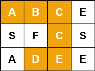
Input: board = [["A","B","C","E"],["S","F","C","S"],["A","D","E","E"]], word = "ABCCED" Output: true
Example 2:
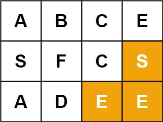
Input: board = [["A","B","C","E"],["S","F","C","S"],["A","D","E","E"]], word = "SEE" Output: true
Example 3:

Input: board = [["A","B","C","E"],["S","F","C","S"],["A","D","E","E"]], word = "ABCB" Output: false
Constraints:
m =board.length=n = board[i].length1 <m, n <= 6=1 <word.length <= 15=boardandwordconsists of only lowercase and uppercase English letters.
Follow up: Could you use search pruning to make your solution faster
with a larger board?
※ 2.10.7.1. Constraints and Edge Cases
- allowed directions are only N,S,E,W so no diagonals
※ 2.10.7.2. My Solution (Code)
This is the optimal code:
1: class Solution: 2: │ def exist(self, board: List[List[str]], word: str) -> bool: 3: │ │ ROWS, COLS = len(board), len(board[0]) 4: │ │ 5: │ │ def backtrack(r, c, k): 6: │ │ │ if k == len(word): 7: │ │ │ │ return True 8: │ │ │ if (r < 0 or r >= ROWS or 9: │ │ │ │ c < 0 or c >= COLS or 10: │ │ │ │ board[r][c] != word[k]): 11: │ │ │ │ return False 12: │ │ │ temp, board[r][c] = board[r][c], "#" # mark as visited 13: │ │ │ 14: │ │ │ # careful on the valid direction: 15: │ │ │ for dr, dc in [(-1,0),(1,0),(0,-1),(0,1)]: 16: │ │ │ │ if backtrack(r + dr, c + dc, k + 1): 17: │ │ │ │ │ # undo the temp overwrite: 18: │ │ │ │ │ board[r][c] = temp 19: │ │ │ │ │ 20: │ │ │ │ │ return True 21: │ │ │ │ │ 22: │ │ │ board[r][c] = temp 23: │ │ │ return False 24: │ │ │ 25: │ │ # allow any cell to be a viable start cell: 26: │ │ for row in range(ROWS): 27: │ │ │ for col in range(COLS): 28: │ │ │ │ if backtrack(row, col, 0): 29: │ │ │ │ │ return True 30: │ │ return False 31:
- Time Complexity:
Let \(m\), \(n\) = board dimensions, \(L\) =
len(word).- Each cell can start a new search: \(O(m * n)\) start positions.
- For each search, you may visit up to \(L\) steps, and at each step at most 4 neighbors.
- In the strictest sense: \(O(m * n * (3^{L}))\)
- (Why 3? After the first letter, movement doesn’t go back to previous cell.)
- Space Complexity:
- Call stack: can go as deep as \(O(L)\) recursion.
- Board is modified in-place (marker), so no extra structures.
※ 2.10.7.2.1. Initial Flawed Versions
The idea is right, some execution misses
1: class Solution: 2: │ def exist(self, board: List[List[str]], word: str) -> bool: 3: │ │ # path will be coordinates 4: │ │ # we can temp mark used with some marker 5: │ │ # fn returns a bool 6: │ │ def backtrack(row, col, path): 7: │ │ │ word_idx = len(path) 8: │ │ │ char = word[word_idx] 9: │ │ │ 10: │ │ │ if board[row][col] != char: 11: │ │ │ │ return False 12: │ │ │ │ 13: │ │ │ if board[row][col] == char and len(path) == len(word): 14: │ │ │ │ return True 15: │ │ │ │ 16: │ │ │ # neighbour generation + neighbour validity check: 17: │ │ │ valid_coords = [(row + dy, col + dx) for dx in range(-1, 2) for dy in range(-1, 2) if 0 <= row + dy < len(board[0]) and 0 <= col + dx < len(board[0][0]) and board[row + dy][col + dx] != "X"] 18: │ │ │ 19: │ │ │ for row_idx, col_idx in valid_coords: 20: │ │ │ │ # choose: 21: │ │ │ │ path.append((row_idx, col_idx)) 22: │ │ │ │ original = board[row][col] 23: │ │ │ │ # mark as used to avoid adding it into search space: 24: │ │ │ │ board[row][col] = "X" 25: │ │ │ │ if backtrack(row_idx, col_idx, path): 26: │ │ │ │ │ return True 27: │ │ │ │ │ 28: │ │ │ │ path.pop() 29: │ │ │ │ board[row][col] = original 30: │ │ │ │ 31: │ │ │ return False 32: │ │ │ 33: │ │ return any(backtrack(start_row, start_col, []) for start_row in range(0, len(board)) for start_col in range(0, len(board[0])))
Improvements:
- just have a fixed
ROW, COLS = len(board), len(board[0])that you can keep referring to - neighbour generation and neighbour validity can be split instead of being the same expression
- neighbour generation: my version allows extra diagonals, that doesn’t follow the question constraints
- base case: just return if
word_idx =len(word)=
- path isn’t actually needed here
1: class Solution: 2: │ def exist(self, board: List[List[str]], word: str) -> bool: 3: │ │ ROWS, COLS = len(board), len(board[0]) 4: │ │ 5: │ │ def backtrack(row, col, word_idx): 6: │ │ │ # If completed the word, return True 7: │ │ │ if word_idx == len(word): 8: │ │ │ │ return True 9: │ │ │ # Out of bounds or already visited or char does not match 10: │ │ │ if (row < 0 or row >= ROWS or 11: │ │ │ │ col < 0 or col >= COLS or 12: │ │ │ │ board[row][col] != word[word_idx]): 13: │ │ │ │ return False 14: │ │ │ │ 15: │ │ │ # Mark the cell as visited 16: │ │ │ temp = board[row][col] 17: │ │ │ board[row][col] = "X" 18: │ │ │ # Try all four directions 19: │ │ │ for dx, dy in [(-1,0),(1,0),(0,-1),(0,1)]: 20: │ │ │ │ if backtrack(row + dx, col + dy, word_idx + 1): 21: │ │ │ │ │ board[row][col] = temp 22: │ │ │ │ │ return True 23: │ │ │ board[row][col] = temp 24: │ │ │ return False 25: │ │ │ 26: │ │ # allow any cell to be the starting point 27: │ │ for start_row in range(ROWS): 28: │ │ │ for start_col in range(COLS): 29: │ │ │ │ if backtrack(start_row, start_col, 0): # start search at each cell 30: │ │ │ │ │ return True 31: │ │ │ │ │ 32: │ │ return False
※ 2.10.7.3. My Approach/Explanation
Similar decision tree searching.
We just need to mark the usage as we recurse down to reduce the search space.
※ 2.10.7.4. My Learnings/Questions
- the neighbour generation have to be careful!
- here, the path use was not necessary
- Alternatives / Extensions:
- Trie-Based Solution (for MANY words):
- For problems like Word Search II (multiple words to seek), build a Trie of all words, then DFS from each cell, pruning whenever the current path is not a prefix.
- Prunes search space substantially in large multi-word queries.
- Bitmask for Visited State (for very large boards): Use an integer or 2D bitmap for visited, but with current constraints, in-place marking is fastest and simplest.
- DFS iterative but too complex to implement the logic for that.
- Trie-Based Solution (for MANY words):
In a recursive approach, boundary checks should always be first before accessing the board cell.
Boundary checks: Always best practice to put them at the start of the function, before any further logic.
QQ: why is it not better to do the validity check before we do the recursive call? wouldn’t we help save the overheads from extra function calls?
AA: Answer: In this problem, the only way a neighbor “becomes” invalid (out of bounds, already visited, wrong char, etc.) is by definition of the recursive function’s base case.
The function is short; overhead is minimal.
Putting the check inside recursion, rather than before calling, keeps the core logic very simple and DRY (don’t repeat yourself). Otherwise, you would need to repeat all criteria in every caller.
Performance-wise, due to Python’s function call overhead, you could check up front, but the difference is tiny for this problem’s input size.
Readability and simplicity usually outweigh the marginal gain:
QQ: Follow up: search pruning for larger boards also answer the extension question in the original problem
AA: Answer: For this single-word search, you could do a small optimization by first scanning the whole board to ensure all letters in word are present in sufficient quantity. If not, return False early.
For MUCH larger problems or when searching many words at once, use a Trie:
- Build a Trie of all target words.
- For each cell, DFS along prefixes in the Trie, pruning paths that are not prefixes.
- This allows one DFS to efficiently search for multiple words (see LeetCode 212: Word Search II).
※ 2.10.7.5. Retros
※ 2.10.7.5.1.
Okay some speed learnings:
for all the grid movement directionality stuff, don’t use generators and all, just use for loop iterators. We want to avoid the CREATION of extra generators for every loop of the backtracked function.
very fast solution:
Show/Hide Python Code1: 2: class Solution: 3: │ def exist(self, board: List[List[str]], word: str) -> bool: 4: │ │ ROWS, COLS = len(board), len(board[0]) 5: │ │ 6: │ │ def backtrack(r, c, k): 7: │ │ │ if k == len(word): 8: │ │ │ │ return True 9: │ │ │ if (r < 0 or r >= ROWS or 10: │ │ │ │ c < 0 or c >= COLS or 11: │ │ │ │ board[r][c] != word[k]): 12: │ │ │ │ return False 13: │ │ │ temp, board[r][c] = board[r][c], "#" # mark as visited 14: │ │ │ 15: │ │ │ # careful on the valid direction: 16: │ │ │ for dr, dc in [(-1,0),(1,0),(0,-1),(0,1)]: 17: │ │ │ │ if backtrack(r + dr, c + dc, k + 1): 18: │ │ │ │ │ # undo the temp overwrite: 19: │ │ │ │ │ board[r][c] = temp 20: │ │ │ │ │ 21: │ │ │ │ │ return True 22: │ │ │ │ │ 23: │ │ │ board[r][c] = temp 24: │ │ │ return False 25: │ │ │ 26: │ │ # allow any cell to be a viable start cell: 27: │ │ for row in range(ROWS): 28: │ │ │ for col in range(COLS): 29: │ │ │ │ if backtrack(row, col, 0): 30: │ │ │ │ │ return True 31: │ │ return False 32: │ │ 33:
slow solution:
Show/Hide Python Code1: class Solution: 2: │ def exist(self, board: List[List[str]], word: str) -> bool: 3: │ │ ROWS, COLS = len(board), len(board[0]) 4: │ │ DIRS = [(1, 0), (-1, 0), (0, 1), (0, -1)] 5: │ │ n = len(word) 6: │ │ 7: │ │ # early exit just incase 8: │ │ if (ROWS * COLS < n): 9: │ │ │ return False 10: │ │ │ 11: │ │ def backtrack(row, col, idx): 12: │ │ │ # endstates: 13: │ │ │ if idx == n: 14: │ │ │ │ return True 15: │ │ │ │ 16: │ │ │ # validity checks: 17: │ │ │ if is_invalid:=(not (0 <= row < ROWS and 0 <= col < COLS) or not board[row][col] == word[idx]): 18: │ │ │ │ return False 19: │ │ │ │ 20: │ │ │ tmp, board[row][col] = board[row][col], "*" 21: │ │ │ # choose from choices: 22: │ │ │ for n_r, n_c in ((row + dr, col + dc) for dr, dc in DIRS): 23: │ │ │ │ if found:=(backtrack(n_r, n_c, idx + 1)): 24: │ │ │ │ board[row][col] = tmp 25: │ │ │ │ │ return found 26: │ │ │ │ │ 27: │ │ │ board[row][col] = tmp 28: │ │ │ 29: │ │ │ return False 30: │ │ │ 31: │ │ for r in range(ROWS): 32: │ │ │ for c in range(COLS): 33: │ │ │ │ if backtrack(r, c, 0): 34: │ │ │ │ │ return True 35: │ │ return False
※ 2.10.8. [70] Palindrome Partitioning (131) almost partitioning pruning
Given a string s, partition s such that every substring of the
partition is a palindrome. Return all possible palindrome
partitioning of s.
Example 1:
Input: s = "aab" Output: [["a","a","b"],["aa","b"]]
Example 2:
Input: s = "a" Output: [["a"]]
Constraints:
1 <s.length <= 16=scontains only lowercase English letters.
※ 2.10.8.1. Constraints and Edge Cases
<list constraints, input limits, or tricky edge cases here>
※ 2.10.8.2. My Solution (Code)
※ 2.10.8.2.1. Iteration Attempt
This failed to understand the question, I can’t sort it because need to follow substring == contiguous region
1: class Solution: 2: │ def partition(self, s: str) -> List[List[str]]: 3: │ │ res = [] 4: │ │ 5: │ │ def is_palindrome(target:str): 6: │ │ │ return target == target[::-1] 7: │ │ │ 8: │ │ │ 9: │ │ # path is just a string here 10: │ │ def backtrack(start_idx, path): 11: │ │ │ # add to res if path subset is a palindrome 12: │ │ │ if is_palindrome(path): 13: │ │ │ │ res.append(path) 14: │ │ │ │ 15: │ │ │ if start_idx >= len(s): 16: │ │ │ │ return 17: │ │ │ │ 18: │ │ │ for choice_idx in range(start_idx, len(s)): 19: │ │ │ │ # skip siblings 20: │ │ │ │ if choice_idx > start_idx and s[choice_idx] == s[choice_idx - 1]: 21: │ │ │ │ │ continue 22: │ │ │ │ │ 23: │ │ │ │ # choose: 24: │ │ │ │ path += (s[choice_idx]) 25: │ │ │ │ backtrack(choice_idx + 1, path) 26: │ │ │ │ 27: │ │ │ │ # backtrack: 28: │ │ │ │ path = path[:-1] 29: │ │ │ return 30: │ │ │ 31: │ │ # sort for semantic sibling skips 32: │ │ s = "".join(sorted(list(s))) 33: │ │ backtrack(0, "") 34: │ │ 35: │ │ return res
1: class Solution: 2: │ def partition(self, s: str) -> List[List[str]]: 3: │ │ partitions = [] 4: │ │ 5: │ │ def is_palindrome(target:str): 6: │ │ │ return target == target[::-1] 7: │ │ │ 8: │ │ # path is builder of the current paritioning 9: │ │ # all elements in the path should be palindromes already 10: │ │ def backtrack(start_idx, path): 11: │ │ │ if start_idx > len(s): 12: │ │ │ │ partitions.append(path[:]) 13: │ │ │ │ return 14: │ │ │ │ 15: │ │ │ # choice_idx is exclusive right bound 16: │ │ │ for choice_idx in range(start_idx, len(s) + 1): 17: │ │ │ │ choice = s[start_idx:choice_idx] 18: │ │ │ │ if not is_palindrome(choice): 19: │ │ │ │ │ continue 20: │ │ │ │ # choose it: 21: │ │ │ │ path.append(choice) 22: │ │ │ │ backtrack(choice_idx + 1, path) 23: │ │ │ │ 24: │ │ │ │ # backtrack: 25: │ │ │ │ path.pop() 26: │ │ │ │ 27: │ │ backtrack(0, []) 28: │ │ 29: │ │ return partitions
Problems:
base condition: suppose
start_idxis for the first possible choice of doing a “yes, partition” then whenstart_idx =len(s)= then we’ve reached the final “partition slot” and we have to take it. It’s already a valid partition.That’s why we need to register/record this current partitions
Off-by-one error in the recursive call: Problem:
choice_idxis the exclusive upper bound, so after slicings[start_idx:choice_idx], the next substring should start atchoice_idx, notchoice_idx + 1.Fix: You should call
backtrack(choice_idx, path), notbacktrack(choice_idx + 1, path).clearer loop ranges
range(start_idx, len(s) + 1)so sub-strings include up to and including the full string.can be clearer still
If we do minor tweaks to this, it will work:
1: class Solution: 2: │ def partition(self, s: str) -> List[List[str]]: 3: │ │ partitions = [] 4: │ │ 5: │ │ def is_palindrome(target:str): 6: │ │ │ return target == target[::-1] 7: │ │ │ 8: │ │ # path is builder of the current paritioning 9: │ │ # all elements in the path should be palindromes already 10: │ │ def backtrack(start_idx, path): 11: │ │ │ if start_idx == len(s): 12: │ │ │ │ partitions.append(path[:]) 13: │ │ │ │ return 14: │ │ │ │ 15: │ │ │ # choice_idx is exclusive right bound, that's why the left range is start_idx + 1 16: │ │ │ for choice_idx in range(start_idx + 1, len(s) + 1): 17: │ │ │ │ choice = s[start_idx:choice_idx] 18: │ │ │ │ if not is_palindrome(choice): 19: │ │ │ │ │ continue 20: │ │ │ │ # choose it: 21: │ │ │ │ path.append(choice) 22: │ │ │ │ backtrack(choice_idx, path) 23: │ │ │ │ # backtrack: 24: │ │ │ │ path.pop() 25: │ │ │ │ 26: │ │ backtrack(0, []) 27: │ │ 28: │ │ return partitions
Fixing the problems gives us this:
1: class Solution: 2: │ def partition(self, s: str) -> List[List[str]]: 3: │ │ partitions = [] 4: │ │ 5: │ │ def is_palindrome(target:str): 6: │ │ │ return target == target[::-1] 7: │ │ │ 8: │ │ # path is builder of the current paritioning 9: │ │ # all elements in the path should be palindromes already 10: │ │ def backtrack(start_idx, path): 11: │ │ │ if start_idx == len(s): 12: │ │ │ │ partitions.append(path[:]) 13: │ │ │ │ return 14: │ │ │ │ 15: │ │ │ # choice_idx is exclusive right bound 16: │ │ │ for choice_idx in range(start_idx + 1, len(s) + 1): 17: │ │ │ │ choice = s[start_idx:choice_idx] 18: │ │ │ │ if not is_palindrome(choice): 19: │ │ │ │ │ continue 20: │ │ │ │ # choose it: 21: │ │ │ │ path.append(choice) 22: │ │ │ │ backtrack(choice_idx, path) 23: │ │ │ │ # backtrack: 24: │ │ │ │ path.pop() 25: │ │ │ │ 26: │ │ backtrack(0, []) 27: │ │ 28: │ │ return partitions 29:
And we can polish it slightly to be:
1: class Solution: 2: │ def partition(self, s: str) -> List[List[str]]: 3: │ │ result = [] 4: │ │ 5: │ │ def is_palindrome(sub): 6: │ │ │ return sub == sub[::-1] 7: │ │ │ 8: │ │ def backtrack(start, path): 9: │ │ │ if start == len(s): 10: │ │ │ │ result.append(path[:]) 11: │ │ │ │ return 12: │ │ │ │ 13: │ │ │ for end in range(start+1, len(s)+1): 14: │ │ │ │ substr = s[start:end] 15: │ │ │ │ if is_palindrome(substr): 16: │ │ │ │ │ path.append(substr) 17: │ │ │ │ │ backtrack(end, path) 18: │ │ │ │ │ path.pop() 19: │ │ │ │ │ 20: │ │ backtrack(0, []) 21: │ │ return result
※ 2.10.8.2.2. Cache optimisation
So for the palindrome checks, we can try to improve the performance using a lru cache
(or just a dict would be fine as well)
1: from functools import lru_cache 2: 3: class Solution: 4: │ def partition(self, s: str): 5: │ │ partitions = [] 6: │ │ 7: │ │ @lru_cache(None) 8: │ │ def is_palindrome(left: int, right: int) -> bool: 9: │ │ │ # Checks if s[left:right] is a palindrome 10: │ │ │ return s[left:right] == s[left:right][::-1] 11: │ │ │ 12: │ │ def backtrack(start_idx: int, current_partition: list): 13: │ │ │ if start_idx == len(s): 14: │ │ │ │ partitions.append(list(current_partition)) 15: │ │ │ │ return 16: │ │ │ │ 17: │ │ │ for end_idx in range(start_idx + 1, len(s) + 1): 18: │ │ │ │ if is_palindrome(start_idx, end_idx): 19: │ │ │ │ │ current_partition.append(s[start_idx:end_idx]) 20: │ │ │ │ │ backtrack(end_idx, current_partition) 21: │ │ │ │ │ current_partition.pop() 22: │ │ │ │ │ 23: │ │ backtrack(0, []) 24: │ │ return partitions
start_idx: current position in the string to start partitioning
end_idx: the (exclusive) end index for the candidate substring
current_partition: accumulated list of palindromic substrings for the current path
partitions: master list collecting all valid palindrome partitions
※ 2.10.8.3. My Approach/Explanation
- we’re choosing the cut points and just iterating.
- adding things only if it’s a valid palindrome, so the accumulator (path) only consists of palindromes within it.
※ 2.10.8.4. My Learnings/Questions
- optimisations:
- lru cache ( or just straight use of dict ) to avoid the duplicate
is_palindrome()checks for an already-checked string
- lru cache ( or just straight use of dict ) to avoid the duplicate
- the off-by-one gotchas are so annoying:
summary of Off-by-one intuition for palindrome partitioning:
Show/Hide Quotestart_idxis where your next cut starts.choice_idxis exclusive—like all Python slices.Cut from
[start_idx:choice_idx], testing allchoice_idxinrange(start_idx+1, len(s)+1)When
start_idx =len(s)=, you’ve split the whole string (base case!)- idea behind it:
- need to be able to intuit what the variables mean:
start_idx: The starting index for the next substring —i.e., the leftmost position you can partition from at this recursion.choice_idx: the right exclusive bound for the current substring (follows same interval style as python slices)
- because of the definitions,
- Our base case is when
start_idx =len(s)=: This means we’ve partitioned up to (and past) the final character—i.e., the whole string has been broken up into palindromes. - our loop for the choices is actually just choosing the right boundaries, that’s why it’s
range(start_idx + 1, len(s) + 1)instead ofrange(start_idx, len(s) + 1)
- Our base case is when
- need to be able to intuit what the variables mean:
You are very close! These classic recursion/backtracking off-by-one “gotchas” are a rite of passage for everyone.
You’re basically just choosing the “cut points” one after another, and yes, the off-by-ones here are classic recursion headaches
※ 2.10.8.5. [Optional] Additional Context
<e.g., “I struggled with X”, “I want to know about alternative algorithms”, etc.>
※ 2.10.9. [71] Letter Combinations of a Phone Number (17)
Given a string containing digits from 2-9 inclusive, return all
possible letter combinations that the number could represent. Return the
answer in any order.
A mapping of digits to letters (just like on the telephone buttons) is given below. Note that 1 does not map to any letters.

Example 1:
Input: digits = "23" Output: ["ad","ae","af","bd","be","bf","cd","ce","cf"]
Example 2:
Input: digits = "" Output: []
Example 3:
Input: digits = "2" Output: ["a","b","c"]
Constraints:
0 <digits.length <= 4=digits[i]is a digit in the range['2', '9'].
※ 2.10.9.1. Constraints and Edge Cases
- empty input is also valid, so we can early return this.
※ 2.10.9.2. My Solution (Code)
※ 2.10.9.2.1. Optimal Recursive DFS (backtracking)
1: class Solution: 2: │ def letterCombinations(self, digits: str) -> List[str]: 3: │ │ 4: │ │ # early return case, empty input: 5: │ │ if not digits: 6: │ │ │ return [] 7: │ │ │ 8: │ │ char_to_choices = { 9: │ │ │ "2": list("abc"), 10: │ │ │ "3": list("def"), 11: │ │ │ "4": list("ghi"), 12: │ │ │ "5": list("jkl"), 13: │ │ │ "6": list("mno"), 14: │ │ │ "7": list("pqrs"), 15: │ │ │ "8": list("tuv"), 16: │ │ │ "9": list("wxyz"), 17: │ │ } 18: │ │ 19: │ │ combis = [] 20: │ │ 21: │ │ def backtrack(path): 22: │ │ │ if len(path) == len(digits): 23: │ │ │ │ combis.append("".join(path[:])) 24: │ │ │ │ return 25: │ │ │ │ 26: │ │ │ choices = char_to_choices[digits[len(path)]] 27: │ │ │ for choice in choices: 28: │ │ │ │ # choose it: 29: │ │ │ │ path.append(choice) 30: │ │ │ │ backtrack(path) 31: │ │ │ │ 32: │ │ │ │ # backtrack: 33: │ │ │ │ path.pop() 34: │ │ │ │ 35: │ │ backtrack([]) 36: │ │ return combis
- Time and Space Complexity
Let \(n\) =
len(digits).- Time complexity:
- Each digit expands the number of combinations by up to 4 (since “7” and “9” have 4 letters).
- The total number of combinations is at most \(4n\).
- For each combination, building the string takes \(O(n)\) time due to the join.
- So worst-case runtime: \(O(4n * n)\)
- Space complexity:
- Recursion stack: up to \(O(n)\)
- Output: up to \(4n\) strings of length n \(\implies O(n * 4n)\)
- Given the constraint (at most 4 digits), this is very efficient and safe.
- Time complexity:
- python idioms:
Slightly more idiomatic:
Use
"".join(path)(no[:]needed; path is not shared).
※ 2.10.9.2.2. Alternative: Iterative BFS style
We iteratively grow the frontier of combos for each digit.
1: class Solution: 2: │ def letterCombinations(self, digits: str) -> List[str]: 3: │ │ if not digits: 4: │ │ │ return [] 5: │ │ mapping = { 6: │ │ │ "2": "abc", "3": "def", "4": "ghi", "5": "jkl", 7: │ │ │ "6": "mno", "7": "pqrs", "8": "tuv", "9": "wxyz" 8: │ │ } 9: │ │ res = [""] 10: │ │ for digit in digits: 11: │ │ │ tmp = [] 12: │ │ │ for comb in res: 13: │ │ │ │ for ch in mapping[digit]: 14: │ │ │ │ │ tmp.append(comb + ch) 15: │ │ │ res = tmp 16: │ │ return res 17:
※ 2.10.9.3. My Approach/Explanation
- this is great, the key idea here is to just have an options map and for each current node in the decision-tree, use that options map to figure out the pool of choices we can make.
- there’s no need to prune anything from the choices pool
※ 2.10.9.4. My Learnings/Questions
- for the options map creation,
"abc".split()is wrong because it just yields[ "abc" ]. The correct way is to just - for the BFS iterative alternative example, we can start merging the graph ideas as well and use terms like “frontier” now.
※ 2.10.9.5. [Optional] Additional Context
Finally, not JUST the intuition is right – the implementation is too!
※ 2.10.10. [72] ⭐️ N-Queens (51) hard almost redo pruning board matrix chess
The n-queens puzzle is the problem of placing n queens on an n x n
chessboard such that no two queens attack each other.
Given an integer n, return all distinct solutions to the n-queens
puzzle. You may return the answer in any order.
Each solution contains a distinct board configuration of the n-queens’
placement, where 'Q' and '.' both indicate a queen and an empty
space, respectively.
Example 1:
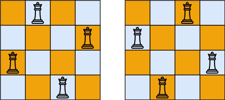
Input: n = 4 Output: [[".Q..","...Q","Q...","..Q."],["..Q.","Q...","...Q",".Q.."]] Explanation: There exist two distinct solutions to the 4-queens puzzle as shown above
Example 2:
Input: n = 1 Output: [["Q"]]
Constraints:
1 <n <= 9=
※ 2.10.10.1. Constraints and Edge Cases
<list constraints, input limits, or tricky edge cases here>
※ 2.10.10.2. My Solution (Code)
※ 2.10.10.2.1. Iterations
I didn’t get the execution right the first time, but I iterated on it. I was close
1: class Solution: 2: │ def solveNQueens(self, n: int) -> List[List[str]]: 3: │ │ # each element is a stringified board 4: │ │ res = [] 5: │ │ 6: │ │ def path_to_board(path): 7: │ │ │ board = [] 8: │ │ │ for row_idx in range(n): 9: │ │ │ │ row = "" 10: │ │ │ │ for col_idx in range(n): 11: │ │ │ │ │ row+= "Q" if (row_idx, col_idx) in path else "." 12: │ │ │ │ board.append(row) 13: │ │ │ return board 14: │ │ │ 15: │ │ def is_valid_placement(r, c, existing_path): 16: │ │ │ for multiplier in range(n): 17: │ │ │ │ diff = multiplier * 1 18: │ │ │ │ up_diff = r - diff 19: │ │ │ │ down_diff = r + diff 20: │ │ │ │ right_diff = c + diff 21: │ │ │ │ left_diff = c - diff 22: │ │ │ │ 23: │ │ │ │ if 0 <= up_diff < n and 0 <= right_diff < n: 24: │ │ │ │ │ top_right = (r - diff, c + diff) 25: │ │ │ │ │ if top_right in existing_path: 26: │ │ │ │ │ │ return False 27: │ │ │ │ │ │ 28: │ │ │ │ if 0 <= up_diff < n and 0 <= left_diff < n: 29: │ │ │ │ │ top_left = (r - diff, c - diff) 30: │ │ │ │ │ if top_left in existing_path: 31: │ │ │ │ │ │ return False 32: │ │ │ │ │ │ 33: │ │ │ │ if 0 <= down_diff < n and 0 <= right_diff < n: 34: │ │ │ │ │ bottom_right = (r + diff, c + diff) 35: │ │ │ │ │ if bottom_right in existing_path: 36: │ │ │ │ │ │ return False 37: │ │ │ │ │ │ 38: │ │ │ │ if 0 <= down_diff < n and 0 <= left_diff < n: 39: │ │ │ │ │ bottom_left = (r + diff, c - diff) 40: │ │ │ │ │ if bottom_left in existing_path: 41: │ │ │ │ │ │ return False 42: │ │ │ │ │ │ 43: │ │ │ return True 44: │ │ │ 45: │ │ # path is a list of queens that we've set 46: │ │ def backtrack(row_idx, path): 47: │ │ │ # done building path, add if valid else ignore 48: │ │ │ if row_idx == n : 49: │ │ │ │ if len(path) == n: 50: │ │ │ │ │ res.append(path_to_board(path)) 51: │ │ │ │ return 52: │ │ │ │ 53: │ │ │ # choices for placement for this row, validity check done here too: 54: │ │ │ choices = [(row_idx, col_idx) for col_idx in range(n) if is_valid_placement(row_idx, col_idx, path)] 55: │ │ │ 56: │ │ │ for choice in choices: 57: │ │ │ │ # choose: 58: │ │ │ │ path.append(choice) 59: │ │ │ │ backtrack(row_idx + 1, path) 60: │ │ │ │ # backtrack: 61: │ │ │ │ path.pop() 62: │ │ │ return 63: │ │ │ 64: │ │ backtrack(0, []) 65: │ │ 66: │ │ return res
Problems:
- Redundant / Over-complicated Diagonal checking
- You generate all four diagonals for every “step” (all multipliers from 0 to n-1) from every queen, searching outwards and checking all reachable diagonal squares.
- In the N-Queens problem (where you always place one queen per row in an incremental order), you only need to check previous rows—never need to check rows after the current one!
- Checking in both directions is not necessary, we can let the search space help improve our efficiency
- With the “one row at a time” method, you only place queens row by row, from top to bottom.
- All possible attacks come from previous rows, so you only need to check upwards diagonals, the same column, and optionally previous rows (actually, you only need to check the diagonals and columns if you’ve already placed queens row by row).
- Inefficient comparisons with existing queen
- Your method checks all multipliers for all four diagonals, causing unnecessary work and making the code error-prone.
It’s a membership check that we care about:
The problem can be solved in \(O(1)\) per check using sets (for columns and diagonals) instead of repeated scans.
- Not checking column unicity
- by placing queens row by row, column collisions are not ruled out except via the path check.
In this case, we want to do the history check via threaded variables, that’s why i overloaded the parameters.
Also we need to keep in mind the trick about how to store diagonals easily
1: class Solution: 2: │ def solveNQueens(self, n: int) -> List[List[str]]: 3: │ │ boards = [] 4: │ │ def format(queens): 5: │ │ │ board = [["." for _ in range(n)] for _ in range(n)] 6: │ │ │ for r, c in queens: 7: │ │ │ │ board[r][c] = 'Q' 8: │ │ │ return ["".join(row) for row in board] 9: │ │ │ 10: │ │ # current board is a set: 11: │ │ # all the queens in curr_board are already valid: 12: │ │ def backtrack(curr_row, curr_queens, curr_cols, curr_pos_diags, curr_neg_diags): 13: │ │ │ if curr_row == n: 14: │ │ │ │ boards.append(format(curr_queens)) 15: │ │ │ │ return 16: │ │ │ │ 17: │ │ │ for r,c in [(curr_row, col_idx) for col_idx in range(n)]: 18: │ │ │ │ # if it matches anything existing 19: │ │ │ │ if c in curr_cols or (r + c) in curr_pos_diags or (r - c) in curr_neg_diags: 20: │ │ │ │ │ continue 21: │ │ │ │ │ 22: │ │ │ │ # choose this: 23: │ │ │ │ curr_queens.append((r,c)) 24: │ │ │ │ curr_cols.add(c) 25: │ │ │ │ curr_pos_diags.add(r + c) 26: │ │ │ │ curr_neg_diags.add(r - c) 27: │ │ │ │ 28: │ │ │ │ # call 29: │ │ │ │ backtrack(curr_row + 1, curr_queens, curr_cols, curr_pos_diags, curr_neg_diags) 30: │ │ │ │ # backtrack: 31: │ │ │ │ curr_queens.pop() 32: │ │ │ │ curr_cols.remove(c) 33: │ │ │ │ curr_pos_diags.remove(r + c) 34: │ │ │ │ curr_neg_diags.remove(r - c) 35: │ │ │ │ 36: │ │ backtrack(0, [], set(), set(), set()) 37: │ │ 38: │ │ return boards
- Let \(n\) be the board size.
- Time complexity:
- The theoretical upper bound is \(O(n!)\) because at each row you might (initially) have \(n\) options, then n−1n−1, etc. The sets and pruning cut many “dead” branches early, but still, worst-case is \(O(n!)\).
- Space complexity:
- Recursion stack: \(O(n)\) (as deep as the board height)
- Sets/lists: \(O(n)\) (for each of columns, pos and neg diagonals, and the queen positions)
- Results: up to the number of valid solutions × \(O(n^{2})\) for the output boards
- Time complexity:
- For \(n\leq9\), this is well within Python’s execution limits.
We can just track column indices and let the relative idx of that element be the row value. This follows the row-by-row approach that we’ve been using.
1: class Solution: 2: │ def solveNQueens(self, n: int) -> List[List[str]]: 3: │ │ res = [] 4: │ │ def build(cols): 5: │ │ │ return [ 6: │ │ │ │ # using a generator here is useful 7: │ │ │ │ ''.join('Q' if i == c else '.' for i in range(n)) 8: │ │ │ │ for c in cols 9: │ │ │ ] 10: │ │ │ 11: │ │ def backtrack(row, cols, pos_diag, neg_diag): 12: │ │ │ if row == n: 13: │ │ │ │ res.append(build(cols)) 14: │ │ │ │ return 15: │ │ │ for c in range(n): 16: │ │ │ │ # unsafe positions: 17: │ │ │ │ if c in cols or (row + c) in pos_diag or (row - c) in neg_diag: 18: │ │ │ │ │ continue 19: │ │ │ │ │ 20: │ │ │ │ # use it 21: │ │ │ │ backtrack( 22: │ │ │ │ │ row + 1, 23: │ │ │ │ │ cols + [c], 24: │ │ │ │ │ pos_diag | {row + c}, 25: │ │ │ │ │ neg_diag | {row - c} 26: │ │ │ │ ) 27: │ │ backtrack(0, [], set(), set()) 28: │ │ return res
- Things well done:
- Used sets for \(O(1)\) checks on columns and diagonals.
- Represented board with only a col-index list; row is implicit via recursion depth.
- Used generators/joins for fast row-string creation.
※ 2.10.10.2.2. Alternative: bitmasking solution
1: def solveNQueens(n): 2: │ res = [] 3: │ def dfs(row, cols, diag1, diag2, path): 4: │ │ if row == n: 5: │ │ │ res.append(path[:]) 6: │ │ │ return 7: │ │ for c in range(n): 8: │ │ │ if not (cols & (1<<c)) and not (diag1 & (1<<(row+c))) and not (diag2 & (1<<(row-c+n-1))): 9: │ │ │ │ s = '.'*c + 'Q' + '.'*(n-c-1) 10: │ │ │ │ dfs(row+1, cols|(1<<c), diag1|(1<<(row+c)), diag2|(1<<(row-c+n-1)), path+[s]) 11: │ dfs(0, 0, 0, 0, []) 12: │ return res
Here, each int encodes set membership with bits.
※ 2.10.10.3. My Approach/Explanation
Just see the iterations above.
※ 2.10.10.4. My Learnings/Questions
- TRICK: diagonals on a board can be captured using sets!
- diagonal type 1: positive slope diagonal (bottom left to top-right
/)- For any square
(row, col), all cells on a positive-slope diagonal share the same value forrow + col.
- For any square
- diagonal type 2: negative slope diagonal (top left to bottom-right
\)- For any square
(row, col), all cells on a negative-slope diagonal share the same value forrow - col.
- For any square
- diagonal type 1: positive slope diagonal (bottom left to top-right
Most optimal solutions track three sets: columns, major and minor diagonals.
Some store just the column index per row, rather than (row, col) pairs.
All similar in core logic.
- Also remember strings are immutable so we can’t do
myStr[3] = 'X', so keep the chars as lists and then just join when needed.
※ 2.10.10.5. [Optional] Additional Context
Very close, it’s the tricks in implementation like:
- no need to track rows, that’s implicit
- diagonals can be stored via a single number
these things make or break the implementation, I think it’s just an exposure thing. Pretty happy with myself regardless.
※ 2.10.10.6. Retros
※ 2.10.10.6.1.
I GOT THIS RIGHT AND IN 28MIN!!!!
NO REFERENCE WHATSOEVER. I EVEN HAD A PEE BREAK.
Here’s my solution, with the emplaced comments:
1: class Solution: 2: │ def solveNQueens(self, n: int) -> List[List[str]]: 3: │ │ # board state management: 4: │ │ get_board = lambda: [["."] * n for _ in range(n)] # keep grids, flatten later 5: │ │ ans = [] 6: │ │ 7: │ │ # board state: 8: │ │ # emplacing a queen: to mark the cell as "Q" 9: │ │ # we need to keep track of boards when we finish it. 10: │ │ 11: │ │ 12: │ │ 13: │ │ # path construction (state management): 14: │ │ # keep to one changing dimension ==> we will go from top row to bottom row 15: │ │ # need to keep track of diagonals from TL to BR and TR to BL (2 types of diagonals) 16: │ │ # need to keep track of columns already exploited as well 17: │ │ 18: │ │ boards = [] 19: │ │ 20: │ │ def backtrack(row_idx, cols, diagonals_a, diagonals_b, curr_board): 21: │ │ │ if row_idx >= n: 22: │ │ │ │ # commit the board, create one here: 23: │ │ │ │ board = get_board() 24: │ │ │ │ for (r, c) in curr_board: 25: │ │ │ │ │ board[r][c] = 'Q' 26: │ │ │ │ boards.append(["".join(row) for row in board]) 27: │ │ │ │ return 28: │ │ │ │ 29: │ │ │ # pick this row, what column? 30: │ │ │ for col_idx in range(n): 31: │ │ │ │ if col_idx in cols: # taken col 32: │ │ │ │ │ continue 33: │ │ │ │ diagonal_a, diagonal_b = row_idx + col_idx, row_idx - col_idx 34: │ │ │ │ 35: │ │ │ │ if diagonal_a in diagonals_a: 36: │ │ │ │ │ continue 37: │ │ │ │ │ 38: │ │ │ │ if diagonal_b in diagonals_b: 39: │ │ │ │ │ continue 40: │ │ │ │ │ 41: │ │ │ │ # when to commit? 42: │ │ │ │ 43: │ │ │ │ 44: │ │ │ │ # this is an option, we either pick it or we don't: 45: │ │ │ │ cols.add(col_idx) 46: │ │ │ │ diagonals_a.add(diagonal_a) 47: │ │ │ │ diagonals_b.add(diagonal_b) 48: │ │ │ │ curr_board.add((row_idx, col_idx)) 49: │ │ │ │ backtrack(row_idx + 1, cols, diagonals_a, diagonals_b, curr_board) 50: │ │ │ │ 51: │ │ │ │ # backtrack on it: 52: │ │ │ │ cols.discard(col_idx) 53: │ │ │ │ diagonals_a.discard(diagonal_a) 54: │ │ │ │ diagonals_b.discard(diagonal_b) 55: │ │ │ │ curr_board.discard((row_idx, col_idx)) 56: │ │ │ │ 57: │ │ │ return 58: │ │ │ 59: │ │ backtrack(0, set(), set(), set(), set()) 60: │ │ 61: │ │ return boards
here’s a cleaner version of it
1: from typing import List 2: 3: class Solution: 4: │ def solveNQueens(self, n: int) -> List[List[str]]: 5: │ │ ans = [] 6: │ │ board = [["."] * n for _ in range(n)] 7: │ │ 8: │ │ def backtrack(r: int, cols: set, pos_diag: set, neg_diag: set): 9: │ │ │ if r == n: 10: │ │ │ │ ans.append(["".join(row) for row in board]) 11: │ │ │ │ return 12: │ │ │ │ 13: │ │ │ for c in range(n): 14: │ │ │ │ if c in cols or (r + c) in pos_diag or (r - c) in neg_diag: 15: │ │ │ │ │ continue 16: │ │ │ │ │ 17: │ │ │ │ # place queen 18: │ │ │ │ board[r][c] = "Q" 19: │ │ │ │ cols.add(c) 20: │ │ │ │ pos_diag.add(r + c) 21: │ │ │ │ neg_diag.add(r - c) 22: │ │ │ │ 23: │ │ │ │ backtrack(r + 1, cols, pos_diag, neg_diag) 24: │ │ │ │ 25: │ │ │ │ # remove queen (backtrack) 26: │ │ │ │ board[r][c] = "." 27: │ │ │ │ cols.remove(c) 28: │ │ │ │ pos_diag.remove(r + c) 29: │ │ │ │ neg_diag.remove(r - c) 30: │ │ │ │ 31: │ │ backtrack(0, set(), set(), set()) 32: │ │ return ans
※ 2.10.11. [Depth-1] Sudoku Solver (37) hard sudoku dimension_flattening_index
Write a program to solve a Sudoku puzzle by filling the empty cells.
A sudoku solution must satisfy all of the following rules:
- Each of the digits
1-9must occur exactly once in each row. - Each of the digits
1-9must occur exactly once in each column. - Each of the digits
1-9must occur exactly once in each of the 93x3sub-boxes of the grid.
The '.' character indicates empty cells.
Example 1:
Constraints:
board.length =9=board[i].length =9=board[i][j]is a digit or'.'.- It is guaranteed that the input board has only one solution.
※ 2.10.11.1. Constraints and Edge Cases
- they want inplace changes
- they guarantee there’s an answer => recursive calls need to be short circuited
※ 2.10.11.2. My Solution (Code)
※ 2.10.11.2.1. v0: correct, 30ish mins
I’m so proud of myself.
I got the intuition right, by slowing down and writing the marker comments.
1: class Solution: 2: │ def solveSudoku(self, board: List[List[str]]) -> None: 3: │ │ """ 4: │ │ Do not return anything, modify board in-place instead. 5: │ │ """ 6: │ │ n = 9 7: │ │ 8: │ │ # find what to preproces: 9: │ │ # fill all empty cells. For each empty cell, I will have some options, and I will carry on 10: │ │ # decision tree: level / iteration ==> slot 11: │ │ # need to keep track of the entire board that we are accumulating and we can just read off that board. 12: │ │ # diagonals don't matter 13: │ │ 14: │ │ # preproc: 15: │ │ # the empty slots themselves 16: │ │ ROWS, COLS = 9, 9 17: │ │ empty_slots = [(r, c) for r in range(ROWS) for c in range(COLS) if board[r][c] == '.'] 18: │ │ 19: │ │ res = None 20: │ │ 21: │ │ # backtracking: everythign before slot index will have been emplaced 22: │ │ def backtrack(slot_idx, board): 23: │ │ │ # done filling the slots: 24: │ │ │ if slot_idx >= len(empty_slots): 25: │ │ │ │ return True 26: │ │ │ │ 27: │ │ │ # i want to fill in this slot_idx, what are my options: 28: │ │ │ row, col = slot = empty_slots[slot_idx] 29: │ │ │ row_vals = {board[row][c] for c in range(COLS) if board[row][c] != "."} 30: │ │ │ col_vals = {board[r][col] for r in range(ROWS) if board[r][col] != "."} 31: │ │ │ 32: │ │ │ block_row_start, block_col_start = (row // 3) * 3, (col // 3) * 3 33: │ │ │ block_vals = {board[r][c] for r in range(block_row_start, block_row_start + 3) for c in range(block_col_start, block_col_start + 3) if board[r][c] != "."} 34: │ │ │ 35: │ │ │ # can't fill this in: 36: │ │ │ options = set(str(i) for i in range(1, 10)) - row_vals - col_vals - block_vals 37: │ │ │ if not options: 38: │ │ │ │ return False 39: │ │ │ │ 40: │ │ │ # if not options: 41: │ │ │ for option in options: 42: │ │ │ │ # i pick that option: 43: │ │ │ │ board[row][col] = str(option) 44: │ │ │ │ if backtrack(slot_idx + 1, board): 45: │ │ │ │ │ return True 46: │ │ │ │ │ 47: │ │ │ │ # backtrack on that: 48: │ │ │ │ board[row][col] = "." 49: │ │ │ │ 50: │ │ │ return False 51: │ │ │ 52: │ │ backtrack(0, board)
I visualised the decision tree to be layer by layer where each layer is a bunch of options for a paticular
slot_idxI’m just getting the options each time and if there are None, I reach a deadend in the decision tree traversal.
when I manage to set values for each slot, then I know that I’ve come to my answer, so I return
the short circuiting part was necessary here.
the calculation of block values took some time:
Show/Hide Python Code1: │ │ block_row_start, block_col_start = (row // 3) * 3, (col // 3) * 3 2: │ │ │ block_vals = {board[r][c] for r in range(block_row_start, block_row_start + 3) for c in range(block_col_start, block_col_start + 3) if board[r][c] != "."}
we can precompute the sets instead of building new each time and calculate them when we are building the empty slots: this makes it a lot faster
Show/Hide Python Code1: DIGITS = set("123456789") 2: 3: # Precompute occupied digits for rows, cols, boxes 4: rows = [set() for _ in range(ROWS)] 5: cols = [set() for _ in range(COLS)] 6: boxes = [set() for _ in range(ROWS)] 7: 8: # .. 9: # when building it: 10: │ │ 11: │ │ empty_slots = [] 12: │ │ for r in range(ROWS): 13: │ │ │ for c in range(COLS): 14: │ │ │ │ val = board[r][c] 15: │ │ │ │ if val == ".": 16: │ │ │ │ │ empty_slots.append((r, c)) 17: │ │ │ │ else: 18: │ │ │ │ │ rows[r].add(val) 19: │ │ │ │ │ cols[c].add(val) 20: │ │ │ │ │ boxes[(r//3)*3 + (c//3)].add(val)
※ 2.10.11.2.2. v1: optimal solution:
1: class Solution: 2: │ def solveSudoku(self, board: List[List[str]]) -> None: 3: │ │ """ 4: │ │ Do not return anything, modify board in-place instead. 5: │ │ """ 6: │ │ ROWS, COLS = 9, 9 7: │ │ DIGITS = set("123456789") 8: │ │ 9: │ │ empty_slots = [] 10: │ │ rows, cols, boxes = [set() for _ in range(ROWS)], [set() for _ in range(COLS)], [set() for _ in range(ROWS)] 11: │ │ 12: │ │ # now we preprocess: 13: │ │ for r in range(ROWS): 14: │ │ │ for c in range(COLS): 15: │ │ │ │ val = board[r][c] 16: │ │ │ │ if val == '.': 17: │ │ │ │ │ empty_slots.append((r, c)) 18: │ │ │ │ else: 19: │ │ │ │ │ rows[r].add(val) 20: │ │ │ │ │ cols[c].add(val) 21: │ │ │ │ │ box_idx = ((r // 3) * 3) + (c // 3) # lmao 22: │ │ │ │ │ boxes[box_idx].add(val) 23: │ │ │ │ │ 24: │ │ # now we figure out how to backtrack: 25: │ │ def backtrack(idx=0): 26: │ │ │ # end-state, we aredone: 27: │ │ │ if idx == len(empty_slots): 28: │ │ │ │ return True 29: │ │ │ │ 30: │ │ │ r, c = empty_slots[idx] 31: │ │ │ box_idx = ((r // 3) * 3) + (c // 3) 32: │ │ │ 33: │ │ │ # gather options: 34: │ │ │ options = DIGITS - rows[r] - cols[c] - boxes[box_idx] 35: │ │ │ 36: │ │ │ # pick the option: 37: │ │ │ for option in options: 38: │ │ │ │ board[r][c] = option 39: │ │ │ │ rows[r].add(option) 40: │ │ │ │ cols[c].add(option) 41: │ │ │ │ boxes[box_idx].add(option) 42: │ │ │ │ 43: │ │ │ │ # short circuiting return: 44: │ │ │ │ if backtrack(idx + 1): 45: │ │ │ │ │ return True 46: │ │ │ │ │ 47: │ │ │ │ # else reset: 48: │ │ │ │ board[r][c] = "." 49: │ │ │ │ rows[r].remove(option) 50: │ │ │ │ cols[c].remove(option) 51: │ │ │ │ boxes[box_idx].remove(option) 52: │ │ │ │ 53: │ │ │ return False 54: │ │ │ 55: │ │ backtrack()
※ 2.10.11.3. My Approach/Explanation
See v0 above
※ 2.10.11.4. My Learnings/Questions
- accuracy trick: Block calculations:
have to multiply the thing by 3 as well, so it’s
idx = (block_idx) * num_blocksand this gives
Show/Hide Python Code1: │ │ block_row_start, block_col_start = (row // 3) * 3, (col // 3) * 3 2: │ │ │ block_vals = {board[r][c] for r in range(block_row_start, block_row_start + 3) for c in range(block_col_start, block_col_start + 3) if board[r][c] != "."}
or even better, look at the trick used in the optimal solution, were we flatten it into a single dimension:
get_box_idx = lambda r,c: (r//3) * 3 + (c//3)
Sudoku solving is more on searching (and requiring global search) and that’s why we can’t apply greedy approaches for it.
Summary: Sudoku solving is more naturally framed as constraint satisfaction and backtracking rather than pure greedy, although heuristics inspired by greedy can improve efficiency by ordering variable assignment.
Sudoku solving via backtracking is a search problem, not a classical greedy problem.
Greedy algorithms pick locally optimal choices hoping for a global solution. In Sudoku, greedy can sometimes fill some cells but doesn’t guarantee a full solution due to dependencies.
Backtracking explores all candidate solutions systematically with pruning; it guarantees correctness.
Some techniques in Sudoku solving resemble greedy steps (like filling cells with only one possible value), but the overall solver must backtrack when conflicts arise.
※ 2.10.11.5. [Optional] Additional Context
<e.g., “I struggled with X”, “I want to know about alternative algorithms”, etc.>
※ 2.11. Heap / Priority Queue
| Headline | Time | ||
|---|---|---|---|
| Total time | 4:26 | ||
| Heap / Priority Queue | 4:26 | ||
| [73] Kth Largest Element in a Stream… | 0:13 | ||
| [74] Last Stone Weight (1046) | 0:12 | ||
| [75] K Closest Points to Origin (973) | 0:06 | ||
| [76] ⭐️ Kth Largest Element in an… | 0:04 | ||
| [77] Task Scheduler (621) | 0:40 | ||
| [78] Design Twitter (355) | 0:21 | ||
| [79] Find Median from Data Stream (295) | 2:50 |
※ 2.11.1. General Notes
※ 2.11.1.1. Fundamentals
※ 2.11.1.2. Tricks
- Euclidean distance comparisons: we can just use the squared distances and avoid the sqrt operation. This will allow us to save a lot of resources.
- Quickselect is always an option for us if we want to find “smallest/largest” while partially sorting instead of complete sorting
- Double heap approach is optimal for general data-streams.
- We can pass in a lambda for the nsmallest comparator.
E.g.
return heapq.nsmallest(k, points, key=lambda p: p[0]**2 + p[1]**2)
※ 2.11.1.3. Interesting Extra Things
the stone throwing in the “Last Stone Weight” problem has interesting mathematical foundations in Minimum Subset Sum Difference problems which have a wide range of usage.
Here’s some context on it:
Show/Hide Python Code1: The **Last Stone Weight** problem, while presented as a process of smashing the two largest stones repeatedly, is deeply connected to a classic challenge in computer science and combinatorial optimization: the **Minimum Subset Sum Difference** problem (sometimes called the **Partition Problem**) [2][5][6][9]. This mathematical foundation not only reveals deeper insights into the stone-smashing game's mechanics but also encompasses a family of real-world partitioning problems. 2: 3: ## The Partition Problem and Why It Matters 4: 5: ### Problem Definition 6: 7: Given a set (or multiset) of positive integers, you are asked to: 8: - Split the multiset into two subsets, $$ S_1 $$ and $$ S_2 $$, 9: - Minimize the absolute difference between the sums of these two subsets: $$ | \text{sum}(S_1) - \text{sum}(S_2) | $$ [2][5][9]. 10: 11: #### Example 12: 13: > Input: [1, 6, 11, 14: > Possible partition: S1 = [1][6][5] (sum 12), S2 = (sum 11). Difference: 1 (minimum possible for this set) [2][5]. 15: 16: ### Importance 17: 18: This formulation directly models: 19: - **Load balancing:** Assigning jobs/tasks of different weights to two machines. 20: - **Scheduling:** Ensuring two teams have near-equal workload. 21: - **Resource allocation:** Packing goods into two containers with almost equal weight. 22: - **Cryptography:** Underpins the hardness of some cryptographic schemes [9]. 23: 24: It's also a fundamental theoretical problem, being **NP-complete** in its decision form, and its approximation and variations inform much of the research in pseudo-polynomial time algorithms [9]. 25: 26: ## Last Stone Weight as a Partition Problem 27: 28: ### Connection 29: 30: - Repeatedly smashing the two heaviest stones in the "Last Stone Weight" game is equivalent to **continually reducing the difference** between two subsets of the multiset. 31: - If you simulate all possible smash orders, the *minimal possible weight* of the last remaining stone is precisely the minimum achievable absolute difference between the sums of any two partitions of the original set [5][6][9]. 32: 33: #### Intuitive Example 34: 35: Suppose stones: [2, 7, 4, 1,[8][1]. 36: - The *sequence* of stone smashes, no matter how you order them, can only reduce the set towards its minimal achievable difference (the subset sum difference). 37: - Thus: **lastStoneWeight = min |sum(S1) - sum(S2)| over all partitions.** 38: 39: ## **Algorithmic Solutions** 40: 41: ### 1. **Dynamic Programming (DP): Subset Sum** 42: 43: The most common approach—a direct adaptation of the **Subset Sum Problem** [2][5][8][9]: 44: 45: - Compute the total sum $$ S $$. 46: - Try to find a subset whose sum is as close as possible to $$ \frac{S}{2} $$. 47: - For each element, decide whether to include it in $$ S_1 $$ (otherwise it goes to $$ S_2 $$). 48: - Use a DP array `dp[i][j]` to record whether a subset of the first `i` elements can sum to `j`. 49: 50: #### Key DP Recurrence 51: 52: For `arr[]`: 53: - **State:** `dp[i][j] = True` if sum `j` is achievable with first `i` items. 54: - **Transition:** 55: │ $$ 56: │ dp[i][j] = dp[i-1][j] \quad \text{(don't take arr[i])} 57: │ $$ 58: │ $$ 59: │ dp[i][j] |= dp[i-1][j-arr[i-1]] \quad \text{(take arr[i])} 60: │ $$ 61: │ 62: - Final answer: 63: │ The **minimum** $$ | S - 2 * j | $$ for all achievable `j` in `dp[n][0 .. S//2]` [2][5]. 64: │ 65: #### Example Python Snippet 66: 67: ```python 68: def min_subset_sum_diff(arr): 69: │ S = sum(arr) 70: │ n = len(arr) 71: │ dp = [False] * (S//2 + 1) 72: │ dp[0] = True 73: │ for num in arr: 74: │ │ for j in range(S//2, num - 1, -1): 75: │ │ dp[j] = dp[j] or dp[j - num] 76: │ for j in range(S//2, -1, -1): 77: │ │ if dp[j]: 78: │ │ return S - 2*j 79: ``` 80: 81: #### Time Complexity 82: - **O(n*S)** (pseudo-polynomial: efficient for small weights, intractable for very large numbers). 83: 84: ### 2. **Meet-in-the-Middle (Bitmask DP) and Variants** 85: 86: For larger arrays or tighter constraints, especially when each subset must be the same size ("Partition Array Into Two Arrays to Minimize Sum Difference" [6]): 87: - **Generate all subset sums** via bitmask on halves of the array (split the array, generate all possible subset sums for each half). 88: - For each possible count in the left half, find the closest matching count subset-sum in the right half to minimize the difference [6]. 89: 90: ## **Contrast With Heap Simulation** 91: 92: ### Heap-based Simulation 93: 94: - Implements the stone-smashing process exactly (always removing the two heaviest). 95: - Efficient and correct for the "Last Stone Weight" *as described* in the problem statement. 96: - **However:** Heap simulation gives only *one possible outcome*, but, perhaps surprisingly, that outcome always matches the minimal achievable difference for any partition of the stones. 97: 98: ### DP/Partition-based Approach 99: 100: - Abstracts the "smashing" to choosing subsets, seeking the minimal difference **directly**. 101: - Guarantees the mathematically minimal difference, regardless of the "smashing order". 102: - Useful for problems that demand optimal partitioning, not just simulation. 103: 104: ## **Summary: Why This Matters** 105: 106: - The **Minimum Subset Sum Difference** problem models an **extremely common dilemma**—dividing resources, workloads, or weights *as evenly as possible*. 107: - Its solutions (DP, meet-in-the-middle, exact vs. approximate) are pillars of combinatorial optimization. 108: - Many "simulation" problems, like Last Stone Weight, are **masked forms** of subset/partition problems; understanding this link illuminates new solution strategies and deeper theory. 109: - The connection explains **why the heap approach works**: in smashing the two largest, you're effectively simulating the process of minimizing the partition difference. 110: 111: Understanding both approaches—and recognizing their equivalence and differences—prepares you for a wide array of allocation, partition, and resource-balancing scenarios encountered across theoretical and applied domains [2][5][6][9]. 112: 113: [1] https://www.geeksforgeeks.org/dsa/minimum-subset-sum-difference-problem-with-subset-partitioning/ 114: [2] https://www.geeksforgeeks.org/dsa/partition-a-set-into-two-subsets-such-that-the-difference-of-subset-sums-is-minimum/ 115: [3] https://www.youtube.com/watch?v=GS_OqZb2CWc 116: [4] https://leetcode.com/problems/partition-array-into-two-arrays-to-minimize-sum-difference/ 117: [5] https://www.techiedelight.com/minimum-sum-partition-problem 118: [6] https://algo.monster/liteproblems/2035 119: [7] https://stackoverflow.com/questions/69921958/partition-a-set-into-two-subsets-so-that-the-difference-of-the-sum-is-minimum-an 120: [8] https://www.designgurus.io/course-play/grokking-dynamic-programming/doc/minimum-subset-sum-difference 121: [9] https://en.wikipedia.org/wiki/Partition_problem 122: [10] https://www.youtube.com/watch?v=WJUXGJ4pGtM
※ 2.11.1.4. Sources of Error
※ 2.11.1.4.1. Gotchas in Python Heap Usage
- It’s Always a Min-Heap: Must negate values for max-heap behavior — easy to forget or get sign errors.
- Heap vs. Sorted List: The list maintained by
heapqonly guarantees that the root of the heap (first element) is the smallest; the rest of the list is not fully sorted
- Tuples for Priority: If items are tuples, Python compares element-wise, so
(priority, counter, item)is a common pattern to avoid problems if multiple elements share the same priority (e.g., tie-breaker by counter for stable order) - Custom Objects: Directly pushing objects without defining
__lt__(less-than) will result in errors if Python can’t compare them- For custom classes, either supply tuples
(priority, object)or implement__lt__.
- For custom classes, either supply tuples
- Heap is Not Thread-safe: Use
queue.PriorityQueueif you need thread-safety, but it’s slower Removing Arbitrary Elements:
heapqdoes not support efficient removal of arbitrary elements other than the smallest;solutions require marking elements as “removed” (soft-delete) or rebuilding the heap.
- Updating Priorities: No built-in method to decrease/increase priority except by removing and reinserting the updated tuple/object.
- Returning Original (Insertion) Order needs a tie-breaker: For elements of equal priority, if you want insertion order preserved, add a tie-breaker (like a unique index or counter).
- Heap Invariants: Operations like
heappushandheappopkeep the heap property but do not guarantee that the internal list is fully sorted.
※ 2.11.2. [73] Kth Largest Element in a Stream (703)
You are part of a university admissions office and need to keep track of
the kth highest test score from applicants in real-time. This helps to
determine cut-off marks for interviews and admissions dynamically as new
applicants submit their scores.
You are tasked to implement a class which, for a given integer k,
maintains a stream of test scores and continuously returns the =k=th
highest test score after a new score has been submitted. More
specifically, we are looking for the =k=th highest score in the sorted
list of all scores.
Implement the KthLargest class:
KthLargest(int k, int[] nums)Initializes the object with the integerkand the stream of test scoresnums.int add(int val)Adds a new test scorevalto the stream and returns the element representing thek=^{=th} largest element in the pool of test scores so far.
Example 1:
Input:
[“KthLargest”, “add”, “add”, “add”, “add”, “add”]
[[3, [4, 5, 8, 2]], [3], [5], [10], [9], [4]]
Output: [null, 4, 5, 5, 8, 8]
Explanation:
KthLargest kthLargest = new KthLargest(3, [4, 5, 8, 2]);
kthLargest.add(3); / return 4
kthLargest.add(5); / return 5
kthLargest.add(10); / return 5
kthLargest.add(9); / return 8
kthLargest.add(4); // return 8
Example 2:
Input:
[“KthLargest”, “add”, “add”, “add”, “add”]
[[4, [7, 7, 7, 7, 8, 3]], [2], [10], [9], [9]]
Output: [null, 7, 7, 7, 8]
Explanation:
KthLargest kthLargest = new KthLargest(4, [7, 7, 7, 7, 8, 3]);
kthLargest.add(2); / return 7
kthLargest.add(10); / return 7
kthLargest.add(9); / return 7
kthLargest.add(9); / return 8
Constraints:
0 <nums.length <= 10=41 <k <= nums.length + 1=-10=^{=4}= <= nums[i] <= 10=4-10=^{=4}= <= val <= 10=4- At most
10=^{=4} calls will be made toadd.
※ 2.11.2.1. Constraints and Edge Cases
- whenever we’re accessing the heap, we should do a nullcheck. This is because at the point of init,
k > len(nums).
※ 2.11.2.2. My Solution (Code)
※ 2.11.2.2.1. Iterations
this was the attempt, with the problems annotated within
1: import heapq 2: 3: class KthLargest: 4: │ 5: │ def __init__(self, k: int, nums: List[int]): 6: │ │ # max heap, so negated # ← not actually negated 7: │ │ self.k = k 8: │ │ heapq.heapify(nums) # ← works for min-heap 9: │ │ self.scores = nums 10: │ │ self.ans = heapq.nlargest(k, self.scores)[0] # ← O(n log k), inefficient, unnecessary 11: │ │ 12: │ def add(self, val: int) -> int: 13: │ │ heapq.heappush(self.scores, val) 14: │ │ 15: │ │ if val <= self.ans: 16: │ │ │ return self.ans 17: │ │ │ 18: │ │ self.ans = heapq.nlargest(self.k, self.scores)[0] 19: │ │ return self.ans
Also the shortcut is incorrect
Your “shortcut” using self.ans in add() is incorrect:
- When val <= self.ans, you still need to recompute the kth largest, because adding (or the heap growing past k) can change which is kth.
we just need to keep the top k, not the entire list
however, assuming that the inefficiencies are alright, here’s how to make this approach work :
1: import heapq 2: 3: class KthLargest: 4: │ 5: │ def __init__(self, k: int, nums: list[int]): 6: │ │ self.k = k 7: │ │ self.scores = nums 8: │ │ heapq.heapify(self.scores) 9: │ │ 10: │ def add(self, val: int) -> int: 11: │ │ heapq.heappush(self.scores, val) 12: │ │ # Always compute kth largest freshly (may be inefficient but is correct) 13: │ │ kth_largest = heapq.nlargest(self.k, self.scores)[-1] 14: │ │ return kth_largest 15:
Remember
1: import heapq 2: 3: class KthLargest: 4: │ 5: │ def __init__(self, k: int, nums: List[int]): 6: │ │ self.k = k 7: │ │ heapq.heapify(nums) 8: │ │ 9: │ │ while len(nums) > k: 10: │ │ │ heapq.heappop(nums) 11: │ │ │ 12: │ │ self.heap = nums 13: │ │ # with k elements, the item at heap[0] is the kth largest in the population 14: │ │ 15: │ def add(self, val: int) -> int: 16: │ │ heapq.heappush(self.heap, val) 17: │ │ while (len(self.heap) > self.k): 18: │ │ │ heapq.heappop(self.heap) 19: │ │ │ 20: │ │ return self.heap[0] 21: │ │ 22: # Your KthLargest object will be instantiated and called as such: 23: # obj = KthLargest(k, nums) 24: #
I actually have a short-circuited version for the add function that goes like so:
1: │ def add(self, val: int) -> int: 2: │ │ # short circuit if the heap is filled with k elements and the incoming element is smaller than the kth largest: 3: │ │ if self.heap and len(self.heap) >= self.k and val < self.heap[0]: 4: │ │ │ return self.heap[0] 5: │ │ │ 6: │ │ heapq.heappush(self.heap, val) 7: │ │ while (len(self.heap) > self.k): 8: │ │ │ heapq.heappop(self.heap) 9: │ │ │ 10: │ │ return self.heap[0]
This shortcircuit has a tricky guard because the heap MUST have at least k elements else the guard maybe buggy.
This can be buggy, be careful of that
That’s one of the edge cases to consider.
- Time and Space Complexity Analysis
- Time Complexity: Initialization: \(O(N * \log(N))\) for heapify and at most \(k\) pops, but you can do \(O(N)\) for heapify plus \(O((N−k)logN)\) for excess pops.
add(val): Each call is \(O(logk)\) – heap insert and possibly a pop if the heap is too big.- Space Complexity: \(O(k)\) for the minheap.
- Improvements:
we could have just done a single pop for the
add(). Because we’re always adding one by one, so it’s a single addition each time, and at most a single element more than \(k\)Show/Hide Python Code1: def add(self, val: int) -> int: 2: │ heapq.heappush(self.heap, val) 3: │ if len(self.heap) > self.k: 4: │ │ heapq.heappop(self.heap) 5: │ return self.heap[0]
1: import heapq 2: class KthLargest: 3: │ def __init__(self, k: int, nums: list[int]): 4: │ │ self.k = k 5: │ │ self.heap = nums 6: │ │ heapq.heapify(self.heap) 7: │ │ while len(self.heap) > self.k: 8: │ │ │ heapq.heappop(self.heap) 9: │ │ │ 10: │ def add(self, val: int) -> int: 11: │ │ heapq.heappush(self.heap, val) 12: │ │ if len(self.heap) > self.k: 13: │ │ │ heapq.heappop(self.heap) 14: │ │ return self.heap[0] 15:
※ 2.11.2.3. My Approach/Explanation
They’re asking just to keep a leaderboard of size k, that’s all we need to do.
We can use a minheap for this and keep the size fixed at k. All the values from the population should have a chance to enter the heap so that we can do the ordering automatically.
Based on the heap invariants, the head the heap (root of the heap) is guaranteed to be ordered so the first element is always going to be the \(k^{th}\) largest as long as we keep the size fixed.
※ 2.11.2.4. My Learnings/Questions
- Intuition
- Heap Intuition
- A heap of size k always contains the k largest items seen so far.
- The smallest in the heap is the kth largest.
- Any new value is only relevant if it could displace the current kth largest.
- Heap Intuition
- the edge case of k < len(nums) means that the list needs to be allowed to build up – what an interesting edge case!
- The version using
heapq.nlargest()insideadd()is inefficient (\(O(Nlogk)\) per call) and not suitable for large streams. - Don’t short-circuit: always update the heap, let the structure handle the kth order!
- Alternative approaches
- Balanced BST, multiset or custom data structure to maintain ordering, but you’d still get \(O(logn)\) per operation, and minheap is more compact and idiomatic.
- Insertion sort / repeated sorting is naive and inefficient (\(O(NlogN)\) per add).
- If data is truly massive and persistent, other stream processing techniques (like external memory sorting) could apply, but for normal coding interviews and online judge problems, the heap approach is best
※ 2.11.2.5. [Optional] Additional Context
<e.g., “I struggled with X”, “I want to know about alternative algorithms”, etc.>
※ 2.11.3. [74] Last Stone Weight (1046)
You are given an array of integers stones where stones[i] is the
weight of the i=^{=th} stone.
We are playing a game with the stones. On each turn, we choose the
heaviest two stones and smash them together. Suppose the heaviest two
stones have weights x and y with x < y=. The result of this smash
is:
- If
x =y=, both stones are destroyed, and - If
x !y=, the stone of weightxis destroyed, and the stone of weightyhas new weighty - x.
At the end of the game, there is at most one stone left.
Return the weight of the last remaining stone. If there are no stones
left, return 0.
Example 1:
Input: stones = [2,7,4,1,8,1] Output: 1 Explanation: We combine 7 and 8 to get 1 so the array converts to [2,4,1,1,1] then, we combine 2 and 4 to get 2 so the array converts to [2,1,1,1] then, we combine 2 and 1 to get 1 so the array converts to [1,1,1] then, we combine 1 and 1 to get 0 so the array converts to [1] then that's the value of the last stone.
Example 2:
Input: stones = [1] Output: 1
Constraints:
1 <stones.length <= 30=1 <stones[i] <= 1000=
※ 2.11.3.1. Constraints and Edge Cases
Nothing fancy, no empty cases to handle either.
※ 2.11.3.2. My Solution (Code)
1: import heapq 2: 3: class Solution: 4: │ def lastStoneWeight(self, stones: List[int]) -> int: 5: │ │ # max heap 6: │ │ stones = [-stone for stone in stones] 7: │ │ heapq.heapify(stones) 8: │ │ 9: │ │ while len(stones) > 1: 10: │ │ │ y = -(heapq.heappop(stones)) 11: │ │ │ x = -(heapq.heappop(stones)) 12: │ │ │ if x == y: 13: │ │ │ │ continue 14: │ │ │ if x < y: 15: │ │ │ │ new_stone = y - x 16: │ │ │ │ heapq.heappush(stones, -(new_stone)) 17: │ │ │ │ 18: │ │ return 0 if not stones else -stones[0]
Cleaned up version:
1: import heapq 2: 3: class Solution: 4: │ def lastStoneWeight(self, stones: list[int]) -> int: 5: │ │ stones = [-s for s in stones] 6: │ │ heapq.heapify(stones) 7: │ │ 8: │ │ while len(stones) > 1: 9: │ │ │ first = -heapq.heappop(stones) # Largest 10: │ │ │ second = -heapq.heappop(stones) # Next largest 11: │ │ │ if first != second: 12: │ │ │ │ heapq.heappush(stones, -(first - second)) 13: │ │ │ │ 14: │ │ return -stones[0] if stones else 0
- Time Complexity
- Building the heap: \(O(n)\)
- Each iteration (collision):
- Pop two: \(2×O(log n)\)
- Push (if needed): \(O(log n)\)
- There can be at most \(n-1\) steps (since each collision reduces stone count).
- Total: \(O(n) + O(n log n) = O(n log n)\)
- Space Complexity
- Heap of up to n items: \(O(n)\)
- No extra auxiliary space.
※ 2.11.3.3. My Approach/Explanation
We just keep a max heap by negating at entry and exit of the heap.
Let a while loop handle it.
Carry out the collisions (while loop iteration is a collision).
Return accordingly.
※ 2.11.3.4. My Learnings/Questions
intuition:
“Always combine the two biggest: this is exactly what a max-heap is for.”
Mathematical “Partition” Solution Variant: This stone smashing problem is related to the minimum subset sum difference (partition problem).
- The last possible stone weight is the minimum possible positive difference of a subset partitioning.
- But: The heap simulation is still the practical/expected coding approach and matches the collision rules literally.
- DP partition solutions fit better in variations where the goal is minimum difference rather than smashing process.
Here’s a deeper dive on it
Show/Hide Md CodeThe **Last Stone Weight** problem, while presented as a process of smashing the two largest stones repeatedly, is deeply connected to a classic challenge in computer science and combinatorial optimization: the **Minimum Subset Sum Difference** problem (sometimes called the **Partition Problem**) [2][5][6][9]. This mathematical foundation not only reveals deeper insights into the stone-smashing game's mechanics but also encompasses a family of real-world partitioning problems. ## The Partition Problem and Why It Matters ### Problem Definition Given a set (or multiset) of positive integers, you are asked to: - Split the multiset into two subsets, $$ S_1 $$ and $$ S_2 $$, - Minimize the absolute difference between the sums of these two subsets: $$ | \text{sum}(S_1) - \text{sum}(S_2) | $$ [2][5][9]. #### Example > Input: [1, 6, 11, > Possible partition: S1 = [1][6][5] (sum 12), S2 = (sum 11). Difference: 1 (minimum possible for this set) [2][5]. ### Importance This formulation directly models: - **Load balancing:** Assigning jobs/tasks of different weights to two machines. - **Scheduling:** Ensuring two teams have near-equal workload. - **Resource allocation:** Packing goods into two containers with almost equal weight. - **Cryptography:** Underpins the hardness of some cryptographic schemes [9]. It's also a fundamental theoretical problem, being **NP-complete** in its decision form, and its approximation and variations inform much of the research in pseudo-polynomial time algorithms [9]. ## Last Stone Weight as a Partition Problem ### Connection - Repeatedly smashing the two heaviest stones in the "Last Stone Weight" game is equivalent to **continually reducing the difference** between two subsets of the multiset. - If you simulate all possible smash orders, the *minimal possible weight* of the last remaining stone is precisely the minimum achievable absolute difference between the sums of any two partitions of the original set [5][6][9]. #### Intuitive Example Suppose stones: [2, 7, 4, 1,[8][1]. - The *sequence* of stone smashes, no matter how you order them, can only reduce the set towards its minimal achievable difference (the subset sum difference). - Thus: **lastStoneWeight = min |sum(S1) - sum(S2)| over all partitions.** ## **Algorithmic Solutions** ### 1. **Dynamic Programming (DP): Subset Sum** The most common approach—a direct adaptation of the **Subset Sum Problem** [2][5][8][9]: - Compute the total sum $$ S $$. - Try to find a subset whose sum is as close as possible to $$ \frac{S}{2} $$. - For each element, decide whether to include it in $$ S_1 $$ (otherwise it goes to $$ S_2 $$). - Use a DP array `dp[i][j]` to record whether a subset of the first `i` elements can sum to `j`. #### Key DP Recurrence For `arr[]`: - **State:** `dp[i][j] = True` if sum `j` is achievable with first `i` items. - **Transition:** │ $$ │ dp[i][j] = dp[i-1][j] \quad \text{(don't take arr[i])} │ $$ │ $$ │ dp[i][j] |= dp[i-1][j-arr[i-1]] \quad \text{(take arr[i])} │ $$ │ - Final answer: │ The **minimum** $$ | S - 2 * j | $$ for all achievable `j` in `dp[n][0 .. S//2]` [2][5]. │ #### Example Python Snippet ```python def min_subset_sum_diff(arr): │ S = sum(arr) │ n = len(arr) │ dp = [False] * (S//2 + 1) │ dp[0] = True │ for num in arr: │ │ for j in range(S//2, num - 1, -1): │ │ │ dp[j] = dp[j] or dp[j - num] │ for j in range(S//2, -1, -1): │ │ if dp[j]: │ │ │ return S - 2*j ``` #### Time Complexity - **O(n*S)** (pseudo-polynomial: efficient for small weights, intractable for very large numbers). ### 2. **Meet-in-the-Middle (Bitmask DP) and Variants** For larger arrays or tighter constraints, especially when each subset must be the same size ("Partition Array Into Two Arrays to Minimize Sum Difference" [6]): - **Generate all subset sums** via bitmask on halves of the array (split the array, generate all possible subset sums for each half). - For each possible count in the left half, find the closest matching count subset-sum in the right half to minimize the difference [6]. ## **Contrast With Heap Simulation** ### Heap-based Simulation - Implements the stone-smashing process exactly (always removing the two heaviest). - Efficient and correct for the "Last Stone Weight" *as described* in the problem statement. - **However:** Heap simulation gives only *one possible outcome*, but, perhaps surprisingly, that outcome always matches the minimal achievable difference for any partition of the stones. ### DP/Partition-based Approach - Abstracts the "smashing" to choosing subsets, seeking the minimal difference **directly**. - Guarantees the mathematically minimal difference, regardless of the "smashing order". - Useful for problems that demand optimal partitioning, not just simulation. ## **Summary: Why This Matters** - The **Minimum Subset Sum Difference** problem models an **extremely common dilemma**—dividing resources, workloads, or weights *as evenly as possible*. - Its solutions (DP, meet-in-the-middle, exact vs. approximate) are pillars of combinatorial optimization. - Many "simulation" problems, like Last Stone Weight, are **masked forms** of subset/partition problems; understanding this link illuminates new solution strategies and deeper theory. - The connection explains **why the heap approach works**: in smashing the two largest, you're effectively simulating the process of minimizing the partition difference. Understanding both approaches—and recognizing their equivalence and differences—prepares you for a wide array of allocation, partition, and resource-balancing scenarios encountered across theoretical and applied domains [2][5][6][9]. [1] https://www.geeksforgeeks.org/dsa/minimum-subset-sum-difference-problem-with-subset-partitioning/ [2] https://www.geeksforgeeks.org/dsa/partition-a-set-into-two-subsets-such-that-the-difference-of-subset-sums-is-minimum/ [3] https://www.youtube.com/watch?v=GS_OqZb2CWc [4] https://leetcode.com/problems/partition-array-into-two-arrays-to-minimize-sum-difference/ [5] https://www.techiedelight.com/minimum-sum-partition-problem [6] https://algo.monster/liteproblems/2035 [7] https://stackoverflow.com/questions/69921958/partition-a-set-into-two-subsets-so-that-the-difference-of-the-sum-is-minimum-an [8] https://www.designgurus.io/course-play/grokking-dynamic-programming/doc/minimum-subset-sum-difference [9] https://en.wikipedia.org/wiki/Partition_problem [10] https://www.youtube.com/watch?v=WJUXGJ4pGtM
※ 2.11.4. [75] K Closest Points to Origin (973)
Given an array of points where points[i] = [x=_{=i}=, y=i=]=
represents a point on the X-Y plane and an integer k, return the k
closest points to the origin (0, 0).
The distance between two points on the X-Y plane is the Euclidean
distance (i.e.,
√(x=_{=1}= - x=2=)=2= + (y=1= - y=2=)=2).
You may return the answer in any order. The answer is guaranteed to be unique (except for the order that it is in).
Example 1:
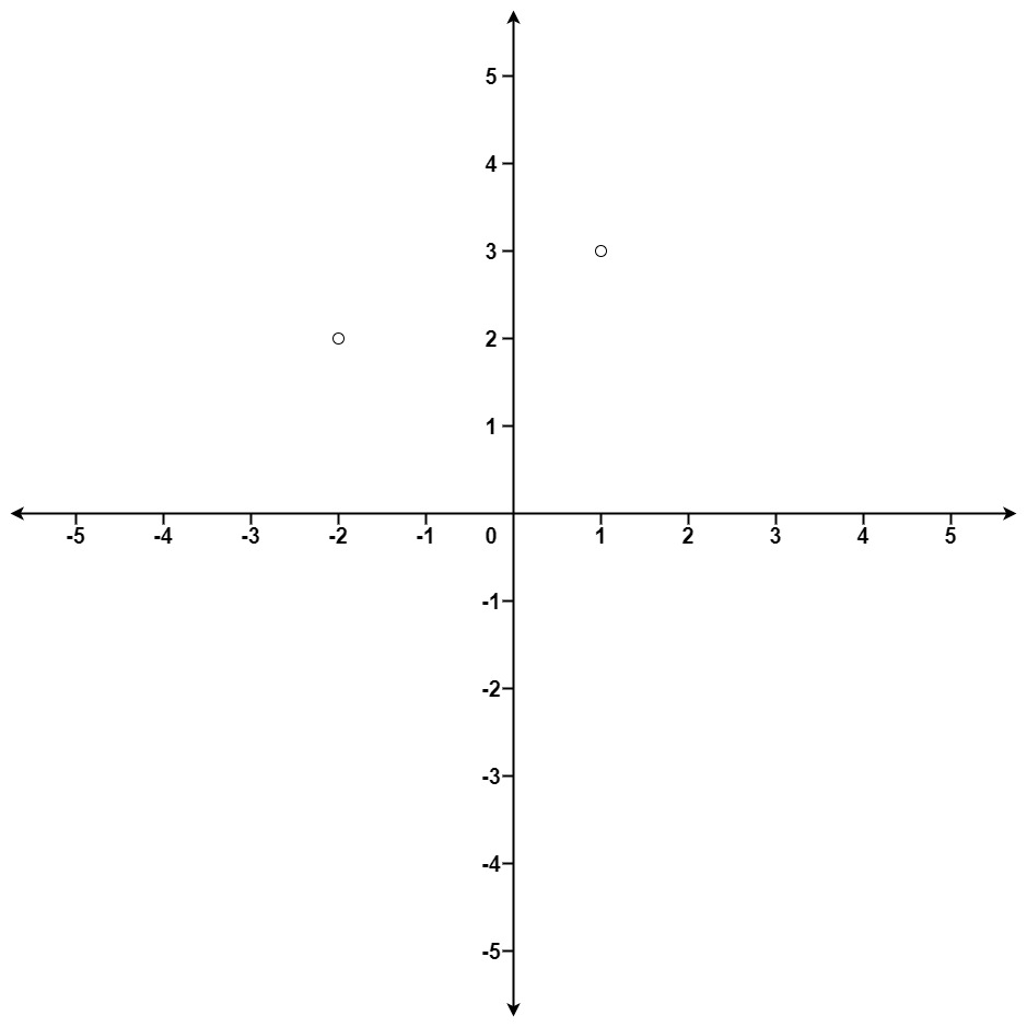
Input: points = [[1,3],[-2,2]], k = 1 Output: [[-2,2]] Explanation: The distance between (1, 3) and the origin is sqrt(10). The distance between (-2, 2) and the origin is sqrt(8). Since sqrt(8) < sqrt(10), (-2, 2) is closer to the origin. We only want the closest k = 1 points from the origin, so the answer is just [[-2,2]].
Example 2:
Input: points = [[3,3],[5,-1],[-2,4]], k = 2 Output: [[3,3],[-2,4]] Explanation: The answer [[-2,4],[3,3]] would also be accepted.
Constraints:
1 <k <= points.length <= 10=4-10=^{=4}= <= x=i=, y=i= <= 10=4
※ 2.11.4.1. Constraints and Edge Cases
- nothing fancy
※ 2.11.4.2. My Solution (Code)
1: import math 2: import heapq 3: 4: class Solution: 5: │ def kClosest(self, points: List[List[int]], k: int) -> List[List[int]]: 6: │ │ points = [(math.sqrt((point[0] ** 2) + (point[1] ** 2)), point) for point in points] 7: │ │ heapq.heapify(points) 8: │ │ 9: │ │ return [tup[1] for tup in heapq.nsmallest(k, points)]
- Time Complexity:
- Calculating distances for all n points: \(O(n)\)
- Building the paired list: \(O(n)\)
heapq.nsmallest(k, ...):- Even though it takes a heap-based approach for small k, in the worst case (large k), it does \(O(n log k)\) operations, so overall:
- \(O(n log k)\)
- So the total is \(O(n log k)\).
- Space Complexity:
- Space for storing pairs: \(O(n)\)
- Space for heap during nsmallest: up to \(O(k)\)
- Output: \(O(k)\)
- Overall: \(O(n)\)
※ 2.11.4.2.1. Optimal (no sqrt, no separate reformatting)
1: import heapq 2: class Solution: 3: │ def kClosest(self, points: list[list[int]], k: int) -> list[list[int]]: 4: │ │ return heapq.nsmallest(k, points, key=lambda p: p[0]**2 + p[1]**2)
looks like we don’t need to heapify this directly first.
※ 2.11.4.2.2. Optimal (maxheap if k << n)
1: import heapq 2: class Solution: 3: │ def kClosest(self, points: list[list[int]], k: int) -> list[list[int]]: 4: │ │ # Maintain a max-heap of size k (heap stores -(distance, point)) 5: │ │ heap = [] 6: │ │ for p in points: 7: │ │ │ dist = -(p[0] ** 2 + p[1] ** 2) 8: │ │ │ if len(heap) < k: 9: │ │ │ │ heapq.heappush(heap, (dist, p)) 10: │ │ │ else: 11: │ │ │ │ heapq.heappushpop(heap, (dist, p)) 12: │ │ return [item[1] for item in heap]
※ 2.11.4.3. My Approach/Explanation
We just keep a minheap and use the order statistics functions (nsmallest()) using that.
※ 2.11.4.4. My Learnings/Questions
- Key TRICK: the sqrt is not needed, we can just use the squared distances and it will be much faster.
- Key Trick: we can pass the lambda to the key for nsmallest!
- Alternatives
Sorting
Simply sort all points by distance and return the first k.
Time: \(O(n log n)\)
Space: \(O(n)\)
Less efficient if \(k << n\).
Quickselect (partial sort) [best possible] Use a variation of the quickselect algorithm to find the k-th smallest distance, then collect all points with distance less than or equal to this.
Average time: \(O(n)\)
Space: \(O(1)\) (in-place, if allowed)
This is optimal for very large n and small k, and is the best possible, but is more elaborate to implement.
※ 2.11.5. [76] ⭐️ Kth Largest Element in an Array (215) redo quick_select_algo
Given an integer array nums and an integer k, return the
k=^{=th} largest element in the array.
Note that it is the k=^{=th} largest element in the sorted order, not
the k=^{=th} distinct element.
Can you solve it without sorting?
Example 1:
Input: nums = [3,2,1,5,6,4], k = 2 Output: 5
Example 2:
Input: nums = [3,2,3,1,2,4,5,5,6], k = 4 Output: 4
Constraints:
1 <k <= nums.length <= 10=5-10=^{=4}= <= nums[i] <= 10=4
※ 2.11.5.1. Constraints and Edge Cases
<list constraints, input limits, or tricky edge cases here>
※ 2.11.5.2. My Solution (Code)
※ 2.11.5.2.1. inferior, pedestrian solution using heapq
Technically this is sorting via a priority queue though
1: import heapq 2: 3: class Solution: 4: │ def findKthLargest(self, nums: List[int], k: int) -> int: 5: │ │ return heapq.nlargest(k, nums)[-1] 6:
Time complexity: \(O(n log k)\) where n = len(nums).
Space complexity: \(O(k)\) for the heap storage.
So if k is large, then it’s better to not use this and to use quickselect.
※ 2.11.5.2.2. correct, easy to understand heapq solution
this uses the API for heapq more expressively
1: import heapq 2: class Solution: 3: def findKthLargest(self, nums, k): 4: heap = [] 5: for num in nums: 6: │ │ if len(heap) < k: 7: │ │ heapq.heappush(heap, num) 8: │ │ else: 9: │ │ if num > heap[0]: 10: │ │ │ │ heapq.heapreplace(heap, num) 11: │ │ │ │ 12: return heap[0]
※ 2.11.5.2.3. optimal solution using quickselect
Quickselect has an average time complexity of \(O(n)\) linear. Space-wise it’s all in place modifications so \(O(1)\) space.
It does the finding without a full sorting.
1: import random 2: from typing import List 3: 4: class Solution: 5: │ def findKthLargest(self, nums: List[int], k: int) -> int: 6: │ │ def quickselect(left, right, target): 7: │ │ │ if left == right: 8: │ │ │ │ return nums[left] 9: │ │ │ pivot_index = random.randint(left, right) 10: │ │ │ # Partition around pivot and return final pivot position 11: │ │ │ new_pivot = partition(left, right, pivot_index) 12: │ │ │ if new_pivot == target: 13: │ │ │ │ return nums[new_pivot] 14: │ │ │ elif new_pivot < target: 15: │ │ │ │ return quickselect(new_pivot + 1, right, target) 16: │ │ │ else: 17: │ │ │ │ return quickselect(left, new_pivot - 1, target) 18: │ │ │ │ 19: │ │ │ │ 20: │ │ def partition(left, right, pivot_index): 21: │ │ │ """ 22: │ │ │ Returns the pivot idx after paritioning left and right segments based on the element values. 23: │ │ │ 24: │ │ │ The property it maintains thereafter is the all to the right of pivot are STRICTLY MORE THAN pivot. 25: │ │ │ 26: │ │ │ All the left of hte pivot are STRICTLY LESS THAN pivot. 27: │ │ │ """ 28: │ │ │ pivot_value = nums[pivot_index] 29: │ │ │ nums[pivot_index], nums[right] = nums[right], nums[pivot_index] 30: │ │ │ store_index = left 31: │ │ │ for i in range(left, right): 32: │ │ │ │ if nums[i] < pivot_value: 33: │ │ │ │ │ nums[store_index], nums[i] = nums[i], nums[store_index] 34: │ │ │ │ │ store_index += 1 35: │ │ │ # move pivot to its final place 36: │ │ │ nums[store_index], nums[right] = nums[right], nums[store_index] 37: │ │ │ 38: │ │ │ return store_index 39: │ │ │ 40: │ │ n = len(nums) 41: │ │ target = n - k # index of k-th largest in sorted order 42: │ │ 43: │ │ return quickselect(0, n - 1, target)
※ 2.11.5.3. My Approach/Explanation
I just gave a pedestrian solution for this.
I can’t imagine a non-sorting approach to this, I’d imagine just doing a partition k times or something.
※ 2.11.5.4. My Learnings/Questions
The optimal average time complexity solution is typically Quickselect, which has expected linear time \(O(n)\). Careful on the use of it though, it should have the index conversion like so: Index conversion
The k-th largest element is at index
len(nums) - kif you sorted in ascending order.Quickselect is meant to find the k-th smallest element: index ksmallest-1
key edge case: Further Issues to Consider
In rare cases of all-equal elements or poor pivots, Quickselect can hit max recursion depth or degrade to \(O(n^{2})\). But with random pivots as shown, this is rare.
- Not sure why I consistently don’t pass the last few edge cases with quickselect implementation. Likely a recursion depth problem so an iterative implementation of quickselect would have worked.
- Classic quickselect works using k-smallest actually:
- Choose a pivot.
- Partition so
left: < pivot,store_index: =pivot=,right: > pivot. - The position of the pivot after partition tells you how many elements are smaller: the pivot is at index p.
- If
p =desired index=, you’ve found your answer.
※ 2.11.5.5. [Optional] Additional Context
※ 2.11.6. [77] Task Scheduler (621) almost redo greedy priority_queue
You are given an array of CPU tasks, each labeled with a letter from A
to Z, and a number n. Each CPU interval can be idle or allow the
completion of one task. Tasks can be completed in any order, but there’s
a constraint: there has to be a gap of at least n intervals between
two tasks with the same label.
Return the minimum number of CPU intervals required to complete all tasks.
Example 1:
Input: tasks = [“A”,“A”,“A”,“B”,“B”,“B”], n = 2
Output: 8
Explanation: A possible sequence is: A -> B -> idle -> A -> B -> idle -> A -> B.
After completing task A, you must wait two intervals before doing A again. The same applies to task B. In the 3rd interval, neither A nor B can be done, so you idle. By the 4th interval, you can do A again as 2 intervals have passed.
Example 2:
Input: tasks = [“A”,“C”,“A”,“B”,“D”,“B”], n = 1
Output: 6
Explanation: A possible sequence is: A -> B -> C -> D -> A -> B.
With a cooling interval of 1, you can repeat a task after just one other task.
Example 3:
Input: tasks = [“A”,“A”,“A”, “B”,“B”,“B”], n = 3
Output: 10
Explanation: A possible sequence is: A -> B -> idle -> idle -> A -> B -> idle -> idle -> A -> B.
There are only two types of tasks, A and B, which need to be separated by 3 intervals. This leads to idling twice between repetitions of these tasks.
Constraints:
1 <tasks.length <= 10=4tasks[i]is an uppercase English letter.0 <n <= 100=
※ 2.11.6.1. Constraints and Edge Cases
<list constraints, input limits, or tricky edge cases here>
※ 2.11.6.2. My Solution (Code)
※ 2.11.6.2.1. Iterations
This aproach is a time-simulation approach. This might work, there might be alternatives to this as well.
- Intent:
- I should have a priority list of factors in descending order of importance e.g. number of jobs left, cooldown, task
- I need to have a PQ such that I get tasks with most number of jobs first, if tied, then least cooldown. If no such element exists, I must have a no-op.
- I keep a counter and just increment it whenever I can and that’s how I eventually can get the priority queue to be empty and all the jobs to have been completed.
1: import heapq 2: from collections import Counter 3: 4: class Solution: 5: │ def leastInterval(self, tasks: List[str], n: int) -> int: 6: │ │ # -freq, wait_for, task 7: │ │ priority = [(-freq, 0, task) for task, freq in Counter(tasks).items()] 8: │ │ heapq.heapify(priority) 9: │ │ 10: │ │ count = 0 11: │ │ 12: │ │ while priority: 13: │ │ │ # check if this needs to be a no-op: 14: │ │ │ is_noop = not any(wait_for == 0 for neg_num_jobs_left, wait_for, task in priority) 15: │ │ │ backlog = [] 16: │ │ │ if is_noop: 17: │ │ │ │ count += 1 18: │ │ │ │ for _ in range(len(priority)): 19: │ │ │ │ │ neg_num_jobs_left, wait_for, task = heapq.heappop(priority) 20: │ │ │ │ │ heapq.heappush(backlog, (neg_num_jobs_left, wait_for - 1, task)) 21: │ │ │ else: 22: │ │ │ │ count += 1 23: │ │ │ │ neg_num_jobs_left, wait_for, task = heapq.heappop(priority) 24: │ │ │ │ # if interval is alright, we do the job now 25: │ │ │ │ if wait_for == 0: 26: │ │ │ │ │ if not neg_num_jobs_left == 0: 27: │ │ │ │ │ │ heapq.heappush(backlog, (neg_num_jobs_left + 1, n, task)) 28: │ │ │ │ # can't do the job: 29: │ │ │ │ else: 30: │ │ │ │ │ heapq.heappush(backlog, (neg_num_jobs_left, wait_for - 1, task)) 31: │ │ │ │ │ 32: │ │ │ priority = backlog[:] 33: │ │ │ 34: │ │ return count
- Problems:
Cooldown Management Bug Problem:
When you idle (no-op), you decrement all
wait_forof all tasks. But when you do a real task, you only update the specific task’s cooldown and potentially add it back with a reset cooldown.Why it’s broken: In a correct simulation, all non-executable tasks have their cooldown decremented every time step—regardless of whether you do an actual job or idle.
But in your code: When you do a task, you forget to decrement the cooldowns for the other tasks for this time step!
Swapping out the whole priority queue as
priority = backlog[:]each loopYou’re creating a new heap list every loop, instead of maintaining a single evolving heap. While this does not break the heap invariant (as long as you use heapq.heappush), it introduces inefficiency by making unnecessary copies and extra memory allocations.
Frequent copying is inefficient and a sign you’re not making best use of the heap’s structure and capabilities.
If you use
heapq.heappushto build backlog (as in your code), then backlog is a valid heap at the end of each loop.Making a shallow copy (with
priority = backlog[:]) simply copies the heap-ordered list; the new priority retains the heap property.The heap invariant is preserved. There’s no step in your code that breaks this property.
Logic when updating job frequencies
When you do a job, you increment
neg_num_jobs_left + 1(since they are stored as negative; correct).However, you only re-add
if not neg_num_jobs_left =0=. But when your counter is negative numbers, that’s only true when it’s 0, which means all jobs for that task are done. That’s fine.Omitted Edge Cases
What if
n=0? Your code still does a bunch of unnecessary prioritizing/idling logic when we can just process all tasks at once.Inefficiency and Complexity
The process is actually a simulation of every time step and can be \(\mathcal{O}(\text{total time} \cdot T)\), which can be larger than the optimal \(\mathcal{O}(N)\) approach.
- Complexity Analysis
- Time: In worst case, at each time unit you re-heapify all tasks. So, worst-case \(O(N^2 \log N)\) (since priority could be up to \(O(N)\) long, and this happens up to \(O(\text{answer})\) times, which can itself be up to \(O(Nn)\) if tasks are spread far apart).
- Space: \(O(N)\) for the heap and any auxiliary structures.
- Shortcomings:
- You’re simulating one step at a time and manually handling all cooldowns and re-heapifying, causing lots of redundant computation.
- Rebuilding the priority queue every loop (priority = backlog[:]) is not optimal heap usage.
- The isnoop approach is correct for the general simulation but is over-complicated for this problem.
- Possible fixes:
- Use two queues: one for available tasks and one for tasks in cooldown (with timestamps).
- Instead of decrementing all cooldowns each time, store the “next valid” time for each cooling task.
1: import heapq 2: from collections import Counter, deque 3: 4: class Solution: 5: │ def leastInterval(self, tasks: List[str], n: int) -> int: 6: │ │ freqs = Counter(tasks) 7: │ │ pq = [(-cnt, task) for task, cnt in freqs.items()] 8: │ │ heapq.heapify(pq) 9: │ │ cooldown = deque() # (ready_time, -cnt, task) 10: │ │ time = 0 11: │ │ while pq or cooldown: 12: │ │ │ time += 1 13: │ │ │ if pq: 14: │ │ │ │ cnt, task = heapq.heappop(pq) 15: │ │ │ │ if cnt + 1: # more left 16: │ │ │ │ │ cooldown.append((time + n, cnt + 1, task)) 17: │ │ │ if cooldown and cooldown[0][0] == time: 18: │ │ │ │ _, next_cnt, next_task = cooldown.popleft() 19: │ │ │ │ heapq.heappush(pq, (next_cnt, next_task)) 20: │ │ return time 21:
You do not actually need to simulate every second or manage explicit cooldowns for fairness. You can get the answer by:
- Greedily picking the most frequent tasks first, and placing them as far apart as needed.
- The “idle time” only needs to be added if some time slots cannot be filled by other tasks.
Formula:
Let:
\(f_{max}=\) frequency of the most common task,
\(n_{max}=\) number of tasks that appear \(f_{max}\) times.
Then : Minimal time = \(\text{max}((f_{max} - 1) \times (n + 1) + n_{max},\text{total tasks})\)
Because you arrange the most frequent tasks in a way that forces at least \(n\) intervals between them.
So the optimal solution to this can be:
1: from collections import Counter 2: 3: class Solution: 4: │ def leastInterval(self, tasks: List[str], n: int) -> int: 5: │ │ freqs = Counter(tasks) 6: │ │ f_max = max(freqs.values()) 7: │ │ n_max = sum(1 for freq in freqs.values() if freq == f_max) 8: │ │ part_len = f_max - 1 9: │ │ empty_slots = part_len * (n + 1) 10: │ │ res = part_len * (n + 1) + n_max 11: │ │ return max(res, len(tasks))
Or to be even more concise:
1: from collections import Counter 2: 3: class Solution: 4: │ def leastInterval(self, tasks: List[str], n: int) -> int: 5: │ │ freq = Counter(tasks).values() 6: │ │ max_freq = max(freq) 7: │ │ num_max = sum(f == max_freq for f in freq) 8: │ │ return max((max_freq - 1) * (n + 1) + num_max, len(tasks))
※ 2.11.6.3. My Approach/Explanation
The intuition here is that for the PQ, we can take the factors that matter to us and have a heapq for it We can manage the cooldowns in a FIFO approach and that’s why we can use the deque.
※ 2.11.6.4. My Learnings/Questions
- python:
- Copying a heapified list preserves the heap property. No need to heapify a copy of a heap.
In Python, a “heap” is just a list with the heap property maintained.
If you copy a list (using
list.copy(),[:], or thelist()constructor), you get a new list with all the elements in the same order as the old one.If the original was a heap, the copy is still a heap (because the order is identical), as long as you don’t modify the new list in a way that breaks heap invariants without using heapq methods.
- This is a greedy problem, just have to make the best choice we can make now
Approach:
We either solve it using the mathematical (counting-based) approach or the time-simulation approach.
The time-simulation approach is my preferred solution because it will apply to the general case and it’s more intuitive.
- Intuition behind the math approach:
Mathematical Intuition
- Tasks with max frequency are the “bottleneck” in the schedule.
- You must ensure at least n intervals between repeats of the most common task.
- Fill all “cooldown slots” with other tasks if you can; otherwise, you must idle.
- The formula computes the time needed if you strictly alternate max-tasks and idle slots, possibly filling them with other tasks, otherwise falling back to the total number of tasks.
- Learnings from the time simulation approach:
- The cooldown queue is good to use
- Intent:
- Use a max heap for available tasks (by remaining count).
- Use a cooldown queue: tasks coming off cooldown after their next valid time.
- At each interval:
- Pop ready tasks, schedule them.
- Move tasks whose cooldown expired back to heap.
- This is more complicated and slower than the math solution but provides insight.
- We can probably just do an early return if
n==0
※ 2.11.6.5. [Optional] Additional Context
The mathematical approach is not intuitive to me.
I should be alright with that because the math approach is more for contests.
※ 2.11.7. [78] Design Twitter (355) K_way_merge
Design a simplified version of Twitter where users can post tweets,
follow/unfollow another user, and is able to see the 10 most recent
tweets in the user’s news feed.
Implement the Twitter class:
Twitter()Initializes your twitter object.void postTweet(int userId, int tweetId)Composes a new tweet with IDtweetIdby the useruserId. Each call to this function will be made with a uniquetweetId.List<Integer> getNewsFeed(int userId)Retrieves the10most recent tweet IDs in the user’s news feed. Each item in the news feed must be posted by users who the user followed or by the user themself. Tweets must be ordered from most recent to least recent.void follow(int followerId, int followeeId)The user with IDfollowerIdstarted following the user with IDfolloweeId.void unfollow(int followerId, int followeeId)The user with IDfollowerIdstarted unfollowing the user with IDfolloweeId.
Example 1:
Input ["Twitter", "postTweet", "getNewsFeed", "follow", "postTweet", "getNewsFeed", "unfollow", "getNewsFeed"] [[], [1, 5], [1], [1, 2], [2, 6], [1], [1, 2], [1]] Output [null, null, [5], null, null, [6, 5], null, [5]] Explanation Twitter twitter = new Twitter(); twitter.postTweet(1, 5); // User 1 posts a new tweet (id = 5). twitter.getNewsFeed(1); // User 1's news feed should return a list with 1 tweet id -> [5]. return [5] twitter.follow(1, 2); // User 1 follows user 2. twitter.postTweet(2, 6); // User 2 posts a new tweet (id = 6). twitter.getNewsFeed(1); // User 1's news feed should return a list with 2 tweet ids -> [6, 5]. Tweet id 6 should precede tweet id 5 because it is posted after tweet id 5. twitter.unfollow(1, 2); // User 1 unfollows user 2. twitter.getNewsFeed(1); // User 1's news feed should return a list with 1 tweet id -> [5], since user 1 is no longer following user 2.
Constraints:
1 <userId, followerId, followeeId <= 500=0 <tweetId <= 10=4- All the tweets have unique IDs.
- At most
3 * 10=^{=4} calls will be made topostTweet,getNewsFeed,follow, andunfollow. - A user cannot follow himself.
※ 2.11.7.1. Constraints and Edge Cases
- the tweet ids will be unique but not necessarily maintaining an order – we need a global counter for tweets
- assume all sequential operations
※ 2.11.7.2. My Solution (Code)
※ 2.11.7.2.1. Iterations
1: from collections import defaultdict 2: import heapq 3: 4: class User: 5: │ def __init__(self, uid=None): 6: │ │ self.id = uid 7: │ │ self.following = set() 8: │ │ 9: class Twitter: 10: │ 11: │ def __init__(self): 12: │ │ self.tweet_count = 0 13: │ │ 14: │ │ self.uid_to_user = defaultdict(User) 15: │ │ 16: │ │ all_tweets = [] 17: │ │ # max heap of elements = (-count, userId, tweetId) 18: │ │ heapq.heapify(all_tweets) 19: │ │ self.all_tweets = all_tweets 20: │ │ 21: │ │ 22: │ def postTweet(self, userId: int, tweetId: int) -> None: 23: │ │ self.tweet_count += 1 24: │ │ heapq.heappush(self.all_tweets, (-self.tweet_count, userId, tweetId)) 25: │ │ 26: │ def getNewsFeed(self, userId: int) -> List[int]: 27: │ │ return heapq.nsmallest(10, self.all_tweets, key=lambda val: val[1] == userId or val[1] in self.uid_to_user[userId].following) 28: │ │ 29: │ def follow(self, followerId: int, followeeId: int) -> None: 30: │ │ self.uid_to_user[followerId].following.add(followeeId) 31: │ │ 32: │ │ 33: │ def unfollow(self, followerId: int, followeeId: int) -> None: 34: │ │ self.uid_to_user[followerId].following.remove(followeeId) 35: │ │ 36: │ │ 37: │ │ 38: │ │ 39: # Your Twitter object will be instantiated and called as such: 40: # obj = Twitter() 41: # obj.postTweet(userId,tweetId) 42: # param_2 = obj.getNewsFeed(userId) 43: # obj.follow(followerId,followeeId) 44: # obj.unfollow(followerId,followeeId)
This uses heapq.merge()
1: from collections import defaultdict 2: import heapq 3: 4: class Twitter: 5: │ 6: │ def __init__(self): 7: │ │ self.tweet_count = 0 8: │ │ # list of tuples (countIdx, tweetId, userId) 9: │ │ self.uid_to_tweets = defaultdict(list) 10: │ │ self.uid_to_following = defaultdict(set) 11: │ │ 12: │ def postTweet(self, userId: int, tweetId: int) -> None: 13: │ │ self.tweet_count += 1 14: │ │ self.uid_to_tweets[userId].append((self.tweet_count, tweetId, userId)) 15: │ │ 16: │ def getNewsFeed(self, userId: int) -> List[int]: 17: │ │ # get following 18: │ │ # ls = *[self.uid_to_tweets[uid] for uid in (self.uid_to_following[userId] | {userId})] 19: │ │ posts = heapq.merge(*[self.uid_to_tweets[uid] for uid in (self.uid_to_following[userId] | {userId})]) 20: │ │ 21: │ │ return [tid for cid, tid, uid in heapq.nlargest(10, posts)] 22: │ │ 23: │ def follow(self, followerId: int, followeeId: int) -> None: 24: │ │ self.uid_to_following[followerId].add(followeeId) 25: │ │ 26: │ │ return 27: │ │ 28: │ │ 29: │ def unfollow(self, followerId: int, followeeId: int) -> None: 30: │ │ self.uid_to_following[followerId].discard(followeeId) 31: │ │ 32: │ │ return 33: │ │ 34: # Your Twitter object will be instantiated and called as such: 35: # obj = Twitter() 36: # obj.postTweet(userId,tweetId) 37: # param_2 = obj.getNewsFeed(userId) 38: # obj.follow(followerId,followeeId) 39: #
Here’s a cleaner version:
1: from collections import defaultdict 2: import heapq 3: 4: class Twitter: 5: │ def __init__(self): 6: │ │ self.tweet_count = 0 7: │ │ self.uid_to_tweets = defaultdict(list) 8: │ │ self.uid_to_following = defaultdict(set) 9: │ │ 10: │ def postTweet(self, userId: int, tweetId: int) -> None: 11: │ │ self.tweet_count += 1 12: │ │ self.uid_to_tweets[userId].append((self.tweet_count, tweetId, userId)) 13: │ │ 14: │ def getNewsFeed(self, userId: int) -> list[int]: 15: │ │ posts = heapq.merge(*(self.uid_to_tweets[uid] 16: │ │ │ │ │ │ │ │ for uid in self.uid_to_following[userId] | {userId})) 17: │ │ │ │ │ │ │ │ 18: │ │ return [post[1] for post in heapq.nlargest(10, posts)] 19: │ │ 20: │ def follow(self, followerId: int, followeeId: int) -> None: 21: │ │ self.uid_to_following[followerId].add(followeeId) 22: │ │ 23: │ def unfollow(self, followerId: int, followeeId: int) -> None: 24: │ │ self.uid_to_following[followerId].discard(followeeId) 25:
Complexity Analysis Consider key methods:
postTweet:
O(1): append to a list.
follow/unfollow:
O(1): set add/discard.
getNewsFeed(userId):
There are at most 500 users.
Merging at most 501 lists (own + all followees) — most will be short, realistically.
heapq.merge is a generators-based merge: to pull k elements from the merged stream is O(k log m) for m input lists IF each list is already sorted.
Then, heapq.nlargest(10, …) actually pulls everything from the merged iterator to find the top 10. In the worst case, if each user and their followees have 10,000 tweets, the newsfeed generation could be up to O(F * T), with F=num followed+1 and T=number of tweets per user (so in pathological test cases, up to ~5,000,000 scan-steps for getNewsFeed, but in practice much less).
This avoids iterating whole lists and guarantees O(#users × log #users × 10) for getNewsFeed.
1: from collections import defaultdict 2: import heapq 3: 4: class Twitter: 5: │ def __init__(self): 6: │ │ self.time = 0 7: │ │ self.user_tweets = defaultdict(list) 8: │ │ self.following = defaultdict(set) 9: │ │ 10: │ def postTweet(self, userId: int, tweetId: int) -> None: 11: │ │ self.time += 1 12: │ │ self.user_tweets[userId].append((self.time, tweetId)) 13: │ │ 14: │ def getNewsFeed(self, userId: int) -> list[int]: 15: │ │ result = [] 16: │ │ # We'll build a heap of (timestamp, tweetId, whose_list, index) 17: │ │ heap = [] 18: │ │ users = self.following[userId].copy() 19: │ │ users.add(userId) 20: │ │ for uid in users: 21: │ │ │ tweets = self.user_tweets[uid] 22: │ │ │ if tweets: 23: │ │ │ │ # push last tweet (most recent), track index 24: │ │ │ │ ts, tid = tweets[-1] 25: │ │ │ │ heapq.heappush(heap, (-ts, tid, uid, len(tweets) - 1)) 26: │ │ while heap and len(result) < 10: 27: │ │ │ ts, tid, uid, idx = heapq.heappop(heap) 28: │ │ │ result.append(tid) 29: │ │ │ if idx > 0: 30: │ │ │ │ prev_ts, prev_tid = self.user_tweets[uid][idx - 1] 31: │ │ │ │ heapq.heappush(heap, (-prev_ts, prev_tid, uid, idx - 1)) 32: │ │ return result 33: │ │ 34: │ def follow(self, followerId: int, followeeId: int): 35: │ │ if followerId != followeeId: 36: │ │ │ self.following[followerId].add(followeeId) 37: │ │ │ 38: │ def unfollow(self, followerId: int, followeeId: int): 39: │ │ self.following[followerId].discard(followeeId)
※ 2.11.7.3. My Approach/Explanation
- just following things, keep a user-specific ordered list so that it can be merged based on followee-ship.
※ 2.11.7.4. My Learnings/Questions
- python:
- nice use of the generators
when using heapq.merge(), we can pass in multiple iterables (sublists) and it will merge them all. The original sublists must be ordered in the first place
QQ: what other conditions need to be met for the heapq.merge() to work well?
AA:
heapq.merge()takes multiple already sorted iterables (lists/streams).Each iterable must be sorted in ascending order (by default comparator or by key, if given — Python 3.5+ allows key, but Leetcode Python is generally older and does not).
If you want to merge by descending order, you must store the items in descending order (e.g., negative timestamps), or just use
heapq.nlargestafter merge as you did.All merged iterables must have comparable elements (e.g., your (timestamp, …) tuples).
The merged output itself is a generator yielding items in merged order (ascending by default).
If any input list is not sorted,
heapq.mergewill produce incorrect output!- when removing from a set, use
discardif the item is not guaranteed to be in the set else there will be aKeyError
※ 2.11.8. [79] Find Median from Data Stream (295) hard double_heap_method
The median is the middle value in an ordered integer list. If the size of the list is even, there is no middle value, and the median is the mean of the two middle values.
- For example, for
arr = [2,3,4], the median is3. - For example, for
arr = [2,3], the median is(2 + 3) / 2 = 2.5.
Implement the MedianFinder class:
MedianFinder()initializes theMedianFinderobject.void addNum(int num)adds the integernumfrom the data stream to the data structure.double findMedian()returns the median of all elements so far. Answers within10=^{-5=} of the actual answer will be accepted.
Example 1:
Input ["MedianFinder", "addNum", "addNum", "findMedian", "addNum", "findMedian"] [[], [1], [2], [], [3], []] Output [null, null, null, 1.5, null, 2.0] Explanation MedianFinder medianFinder = new MedianFinder(); medianFinder.addNum(1); // arr = [1] medianFinder.addNum(2); // arr = [1, 2] medianFinder.findMedian(); // return 1.5 (i.e., (1 + 2) / 2) medianFinder.addNum(3); // arr[1, 2, 3] medianFinder.findMedian(); // return 2.0
Constraints:
-10=^{=5}= <= num <= 10=5- There will be at least one element in the data structure before
calling
findMedian. - At most
5 * 10=^{=4} calls will be made toaddNumandfindMedian.
Follow up:
- If all integer numbers from the stream are in the range
[0, 100], how would you optimize your solution? - If
99%of all integer numbers from the stream are in the range[0, 100], how would you optimize your solution?
※ 2.11.8.1. Constraints and Edge Cases
Nothing fancy here
※ 2.11.8.2. My Solution (Code)
※ 2.11.8.2.1. wrong v1: NO BALANCING
This almost works, except one of the heap can end up getting only the elements.
If we don’t rebalance the entries then it won’t work well.
1: import heapq 2: 3: class MedianFinder: 4: │ def __init__(self): 5: │ │ self.left_max_heap = [] 6: │ │ self.right_min_heap = [] 7: │ │ self.size = 0 8: │ │ 9: │ def addNum(self, num: int) -> None: 10: │ │ curr_med = self.findMedian() 11: │ │ # add to left_max_heap 12: │ │ if num < curr_med: 13: │ │ │ heapq.heappush(self.left_max_heap, -num) 14: │ │ else: 15: │ │ │ heapq.heappush(self.right_min_heap, num) 16: │ │ │ 17: │ │ self.size += 1 18: │ │ 19: │ def findMedian(self) -> float: 20: │ │ if not self.size: 21: │ │ │ return -float('inf') 22: │ │ │ 23: │ │ # odd: 24: │ │ if self.size % 2 != 0: 25: │ │ │ return self.right_min_heap[0] 26: │ │ │ 27: │ │ else: 28: │ │ │ 29: │ │ │ return (self.right_min_heap[0] + (-self.left_max_heap[0])) / 2
- Problems
You never balance the two heaps
The essence of this approach is to keep the sizes of
left_max_heapandright_min_heapwithin 1 of each other, so the median is always at the tops of the heaps.In your code, you only add to one or the other but never do the crucial re-balancing step.
This quickly leads to lopsided heaps and incorrect median calculations.
The use of findMedian is error-prone findMedian can fail/cause error
At the start, or if all elements went to one side (because of bug 1), you might index an empty heap.
For the first insert,
.findMedian()is called before any elements are added, socurr_med = self.findMedian()raisesIndexError.Wrong median logic:
After rebalancing, in standard convention
right_min_heapis allowed to be larger by at most 1 element. But your code assumes if odd size, the median is alwaysright_min_heap, which is only correct if you preserve that property.Since the rebalancing is not happening now, that property is not being maintained.
※ 2.11.8.2.2. correct v2: WITH BALANCING
Fixes from the errors made:
Show/Hide Python Codeimport heapq class MedianFinder: │ def __init__(self): │ │ self.left_max_heap = [] │ │ self.right_min_heap = [] │ │ │ def addNum(self, num: int) -> None: │ │ """ │ │ Approach: │ │ │add to left heap, │ │ │take max from left heap and shift to right heap │ │ │rebalance if necessary │ │ """ │ │ heapq.heappush(self.left_max_heap, -num) │ │ heapq.heappush(self.right_min_heap, -heapq.heappop(self.left_max_heap)) │ │ │ │ # rebalancing step: if right is more than the left beyond + 1 │ │ if len(self.right_min_heap) > len(self.left_max_heap) + 1: │ │ │ heapq.heappush(self.left_max_heap, -heapq.heappop(self.right_min_heap)) │ │ │ │ def findMedian(self) -> float: │ │ # the odd number case: │ │ if len(self.right_min_heap) > len(self.left_max_heap): │ │ │ │ │ │ return float(self.right_min_heap[0]) │ │ │ │ │ # even number case │ │ else: │ │ │ return (self.right_min_heap[0] - self.left_max_heap[0]) / 2.0
- Complexity Analysis
- addNum: \(O(log n)\) per operation (heap push/pop)
- findMedian: \(O(1)\)
- Space: \(O(n)\), all values are stored (half in each heap).
Slightly more common idiom with cleaned up naming
1: import heapq 2: 3: class MedianFinder: 4: │ def __init__(self): 5: │ │ self.small = [] # Max heap (as negative numbers) 6: │ │ self.large = [] # Min heap 7: │ │ 8: │ def addNum(self, num: int) -> None: 9: │ │ # Python heapq is minheap, so push negative for maxheap 10: │ │ heapq.heappush(self.small, -num) 11: │ │ # All numbers in small must be <= numbers in large 12: │ │ heapq.heappush(self.large, -heapq.heappop(self.small)) 13: │ │ # Balance: small can be larger by 1 14: │ │ if len(self.large) > len(self.small): 15: │ │ │ heapq.heappush(self.small, -heapq.heappop(self.large)) 16: │ │ │ 17: │ def findMedian(self) -> float: 18: │ │ if len(self.small) > len(self.large): 19: │ │ │ return -self.small[0] 20: │ │ return (self.large[0] - self.small[0]) / 2.0 21:
※ 2.11.8.2.3. correct (bounded range only)
This only works for bounded range
1: class MedianFinder: 2: │ def __init__(self): 3: │ │ self.freq = [0] * 101 # freq[i]: count of number i in [0,100] 4: │ │ self.count = 0 # total number of inserted values 5: │ │ 6: │ def addNum(self, num: int) -> None: 7: │ │ self.freq[num] += 1 8: │ │ self.count += 1 9: │ │ 10: │ def findMedian(self) -> float: 11: │ │ total = self.count 12: │ │ 13: │ │ # Find the median index(es) (0-based in sorted stream) 14: │ │ if total % 2 == 1: 15: │ │ │ median_pos1 = median_pos2 = total // 2 16: │ │ else: 17: │ │ │ median_pos1 = total // 2 - 1 18: │ │ │ median_pos2 = total // 2 19: │ │ │ 20: │ │ # helps us account for the even cases where we'll have 2 values 21: │ │ result = [] 22: │ │ running_count = 0 23: │ │ for value in range(101): # Loop over all possible values 24: │ │ │ running_count += self.freq[value] 25: │ │ │ # Add value to result if we cross the median positions 26: │ │ │ if len(result) == 0 and running_count > median_pos1: 27: │ │ │ │ result.append(value) 28: │ │ │ if len(result) == 1 and running_count > median_pos2: 29: │ │ │ │ result.append(value) 30: │ │ │ │ break 31: │ │ │ │ 32: │ │ return sum(result) / len(result) 33:
freq: List holding the count of each possible value.count: How many numbers are currently stored.running_count: Used to walk through the “virtual sorted array” and find the median positions.median_pos1/median_pos2: The (zero-based) index or indices (since the median is the average of two for even-length lists) in the virtual sorted stream.
※ 2.11.8.3. My Approach/Explanation
Approach is that we just need to keep an idea of left and right areas near the median.
There are 2 cases:
when the overall size of the nums received is
- odd: only need one element
- take the value from the larger heap
- even
- take a value from left and a value from the right and then average them up
※ 2.11.8.4. My Learnings/Questions
- TRICK: double-heap approach is optimal for general data streams
- The intuition for this comes about as soon as we just write out the examples
- The rebalancing is a natural solution to the problem where it’s lopsided
QQ: what are some optimisations I can do here? e.g. can i have a fixed capacity heap? how does the eviction work? Can I have a fixed capacity heap? How would eviction work?
AA: No.
The whole point of the two-heap solution is that, in order to maintain the median at all times, you must know the entire left and right halves of the current data (or at least their roots).
If you keep only the “latest k” (e.g., an LRU) you lose any guarantee you have the real median unless the data stream is known to fit.
For a bounded domain (), use the frequency array!
For a “moving median” window of size k (not this problem), you need a different data structure—like two balanced BST/multisets plus a lazy deletion queue.
- Extension Questions:
- If all integer numbers from the stream are in the range \([0, 100]\), how would you optimize your solution?
- since bounded domains, we can do frequency counting (see the counting solution above)
99% in the range Bucket in freq array, store the rare outliers in a secondary data structure (e.g., another heap or BST).
Fast median finding still, but extra logic to handle cases where the true median actually falls outside the range.
- If all integer numbers from the stream are in the range \([0, 100]\), how would you optimize your solution?
※ 2.11.8.5. [Optional] Additional Context
- I had gotten really tired and motivation was low. Taking a break was absolutely necessary so that I don’t end up cache-thrashing and wasting all the questions that I was about to do.
※ 2.12. Graphs
| Headline | Time | ||
|---|---|---|---|
| Total time | 8:06 | ||
| Graphs | 8:06 | ||
| [80] Number of Islands (200) | 0:51 | ||
| [81] Max Area of Island (695) | 0:21 | ||
| [82] Clone Graph (133) | 0:50 | ||
| [83] Walls and Gates (??) | 0:41 | ||
| [84] Rotting Oranges (994) | 0:23 | ||
| [85] ⭐️ Pacific Atlantic Water Flow… | 1:27 | ||
| [86] Surrounded Regions (130) | 0:38 | ||
| [87] Course Schedule I (207) | 0:17 | ||
| [88] Course Schedule II (210) | 0:22 | ||
| [89] Graph Valid Tree (??) | 0:14 | ||
| [90] Number of Connected Components… | 0:21 | ||
| [91] ⭐️ Redundant Connection (684) | 0:20 | ||
| [92] Word Ladder (127) | 1:21 |
※ 2.12.1. General Notes
※ 2.12.1.1. Fundamentals
※ 2.12.1.1.1. Detecting Bipartite Graphs
Just a basic primitive on what we can do for bi-partite checks. We can phrase this as a graph colouring question where we just have 2 colours to colour every graph with.
So this is a traversal problem, we try to use only two colours so that no connected nodes have the same colour.
DFS is more common:
1: class Solution: 2: │ def isBipartite(self, graph: List[List[int]]) -> bool: 3: │ │ color = [0] * len(graph) # Map node i -> odd=1, even=-1 4: │ │ stack = [] 5: │ │ 6: │ │ for i in range(len(graph)): 7: │ │ │ if color[i] != 0: # already coloured 8: │ │ │ │ continue 9: │ │ │ color[i] = -1 # set initial state, consider it as a source for the DFS 10: │ │ │ 11: │ │ │ stack.append(i) 12: │ │ │ while stack: # DFS through 13: │ │ │ │ node = stack.pop() 14: │ │ │ │ for nei in graph[node]: 15: │ │ │ │ │ if color[node] == color[nei]: # clashing colours 16: │ │ │ │ │ │ return False 17: │ │ │ │ │ elif not color[nei]: # uncoloured, time to colour it 18: │ │ │ │ │ │ stack.append(nei) 19: │ │ │ │ │ │ color[nei] = -1 * color[node] # alternative it 20: │ │ │ │ │ │ 21: │ │ return True
When we want to track many:many relations between two dimensions (e.g. actors and movies )
※ 2.12.1.1.2. Cycle Detection
key problem to solve is: do I have a cycle in my graph?
- To check if there’s a cycle, we need to consider a general cycle (more than just immediate link-back).
This means that we’d need some way to encode 3 states for nodes.
We can encode them in any way we want, just need 3 states:
- Unvisited
- Visiting (currently, in this branch exploration)
- Visited (when leaving it)
- During DFS, if you encounter a node marked as Visiting in the current path, a cycle exists.
This is the DFS with Recursion stack, just that the mental model we’re using here is that we’re colouring nodes to signal the 3 states.
Purely just a framing of the approach here.
If not all nodes are processed (cannot remove all nodes with in-degree 0), the remaining nodes form a cycle.
- Each node starts in its own set.
- For every edge, check if the two ends have the same parent:
- If yes, adding the edge would create a cycle.
- If no, unite their sets.
- Note: Standard Union-Find does not directly apply to directed graph cycle detection.
- Track the parent node on DFS traversal.
- If you REVISIT a neighbor that is not the parent of the current node, you have a cycle.
※ 2.12.1.1.3. Topological Sorting Algorithms
- For every unvisited node, perform a DFS.
- On exit (i.e., after exploring all descendants), push the node to a stack or prepend it to an output list.
- The resulting list (reversed) is the topological order.
- Calculate the in-degree for each node.
- Start with all nodes of in-degree 0 (no prerequisites).
- While the queue is not empty:
- Pop a node, add it to the topo order.
- For each outgoing edge to neighbor:
- Decrement neighbor’s in-degree.
- If in-degree becomes 0, enqueue neighbor.
- If you cannot include all nodes, the graph contains a cycle.
1: from collections import defaultdict, deque 2: from typing import List 3: 4: def kahn_topological_sort(num_nodes: int, edges: List[List[int]]) -> List[int]: 5: │ """ 6: │ Generic Kahn’s Algorithm for Topological Sorting. 7: │ 8: │ Args: 9: │ │ num_nodes: number of vertices (0 to num_nodes-1) 10: │ │ edges: list of [u, v] meaning there is a directed edge u → v 11: │ │ 12: │ Returns: 13: │ │ topo_order: A list of vertices in topologically sorted order. 14: │ │ If there is a cycle, returns an empty list. 15: │ """ 16: │ # Step 1: Build adjacency list and in-degree array 17: │ adj = defaultdict(list) 18: │ in_degree = [0] * num_nodes 19: │ 20: │ for u, v in edges: 21: │ │ adj[u].append(v) 22: │ │ in_degree[v] += 1 23: │ │ 24: │ # Step 2: Initialize queue with nodes having in-degree 0 25: │ queue = deque([i for i in range(num_nodes) if in_degree[i] == 0]) 26: │ topo_order = [] 27: │ 28: │ # Step 3: Process nodes with in-degree 0 29: │ while queue: 30: │ │ node = queue.popleft() 31: │ │ topo_order.append(node) 32: │ │ 33: │ │ # Reduce in-degree for all neighbors 34: │ │ for neighbor in adj[node]: 35: │ │ │ in_degree[neighbor] -= 1 36: │ │ │ if in_degree[neighbor] == 0: 37: │ │ │ │ queue.append(neighbor) 38: │ │ │ │ 39: │ # Step 4: Check if topological sort is possible (no cycle) 40: │ if len(topo_order) == num_nodes: 41: │ │ return topo_order # Valid topological order 42: │ else: 43: │ │ return [] # Cycle detected → no valid topological ordering
- Variant of Kahn’s algorithm.
- Instead of an ordinary queue, use a priority queue (min-heap or max-heap) to always select the lex smallest/largest in-degree 0 node.
- Useful when a specific order is required (e.g., lexicographically smallest topological order).
- Recursively:
- For all available in-degree 0 nodes at the current step:
- Add node to partial order, decrease in-degrees accordingly.
- Recurse.
- Backtrack.
- For all available in-degree 0 nodes at the current step:
- Generates all possible topological sorts.
- Algorithmic complexity is high (factorial in the number of nodes for highly connected DAGs).
- Maintain adjacency matrix.
- Iteratively remove nodes/columns with all zero entries (no incoming edges).
- The removal order gives a possible topological order.
- Remove all in-degree 0 nodes as a “layer.”
- Repeat on the residual graph.
- Each layer can be processed in parallel.
- Produces a series of layers, not necessarily a linear topo sort (but can be linearized if needed).
| Algorithm | Can Detect Cycles | Produces Topo Order | Notes |
|---|---|---|---|
| DFS with Rec Stack/Coloring | Yes | Yes | Canonical, easy to implement |
| Kahn’s Algorithm (BFS In-degree) | Yes | Yes | Canonical, popular in interviews |
| Modified Kahn’s with Priority Queue | Yes | Yes | For lex order or weighted DAGs |
| Enumerating All Topo Sorts | - | Yes (all orders) | Higher complexity, not often practical |
| Matrix Method | Yes | Sometimes | Theoretical/academic cases |
| Level-based Traversal | - | Layers | Good for parallel processing |
※ 2.12.1.2. Style
- I like the idea of defining
ROWS,COLS,DIRECTIONSat the top and consistently making references to that. - Naming preferences:
neiandneisfor “neighbour”, “neighbours”- careful about not mixing up american and british spellings
※ 2.12.1.3. Tricks
- Character patterns:
- we can use wildcards to get more branched graph (ref “Word Ladder” problem).
for union find, remember that we can amortize our searches by doing path compression when we call the find operation. Th find operation can be written as :
Show/Hide Python Code1: │ │ def find(x): 2: │ │ │ if parent[x] != x: 3: │ │ │ │ # path compression 4: │ │ │ │ parent[x] = find(parent[x]) 5: │ │ │ return parent[x]
there’s rank based optimisation as well, wherein we track the ranks so that we are always joining the smaller tree to the bigger tree (which is asymptotically similar but practically a lot faster)
- Flood fill algorithm:
TRICK: Memory hack: reuse input
we can reuse the input grid for tracking (e.g. in the floodfill approach for “Number of Islands” problem)
TRICK: reduce search space ASAP
to reduce search spaces, we can ensure that any children added to queues / stacks get marked as visited as we insert into the ds, rather than when we retrieve from the DS.
TRICK: to avoid last-scans for completion, use an aux counter number that we can decrement. IF fully decremented, then the overall state is complete, else it’s an incomplete state.
e.g. Rotting Oranges problem.
※ 2.12.1.4. Useful Algorithms
※ 2.12.1.4.1. Kahn’s Algorithm for Topological Sorting
What is? Kahn’s algorithm is a BFS-based way to perform a topological sort on a Directed Acyclic Graph (DAG).
If the graph contains a cycle, the sort cannot be completed for all nodes.
In this problem, “Can you finish all courses?” is equivalent to: Does a valid topological sort exist (is the graph acyclic)?
- Key Intuition
- Kahn’s algorithm “peels off” nodes that are dependencies for others, one layer at a time.
- If you can’t “peel off” all nodes, the graph has a cycle.
- TLDR;
- Use in-degree to know when nodes/courses are ready to take.
- BFS “depletes” requirements.
- Can’t take all = cycle/unsatisfiable.
Logic Just read the code here:
Show/Hide Python Code1: │ │ from collections import defaultdict, deque 2: │ │ 3: │ │ class Solution: 4: │ │ def canFinish(self, numCourses: int, prerequisites: List[List[int]]) -> bool: 5: │ │ # Build adjacency list and in-degree array 6: │ │ adj = defaultdict(list) 7: │ │ 8: │ │ 9: │ │ # in-degree: For each node, count how many edges point to it = how many prerequisites it has. 10: │ │ in_degree = [0] * numCourses 11: │ │ 12: │ │ for course, pre in prerequisites: 13: │ │ adj[pre].append(course) # prereq → course 14: │ │ in_degree[course] += 1 # course needs one more prereq 15: │ │ 16: │ │ # 1. Find all courses with no prerequisites. Any element in the queue is "ready to be taken" 17: │ │ queue = deque([i for i in range(numCourses) if in_degree[i] == 0]) 18: │ │ visited = 0 # How many courses we've "finished" 19: │ │ 20: │ │ # 2. Process all courses "ready" to be taken 21: │ │ while queue: 22: │ │ node = queue.popleft() 23: │ │ # count as finished / visited 24: │ │ visited += 1 25: │ │ 26: │ │ for neighbor in adj[node]: # All courses that depend on this one 27: │ │ in_degree[neighbor] -= 1 # One prereq is now done! 28: │ │ if in_degree[neighbor] == 0: # this neighbor is not ready to be taken 29: │ │ queue.append(neighbor) 30: │ │ 31: │ │ # 3. If we managed to "take" all courses, there is no cycle! 32: │ │ return visited == numCourses
- How can it detect cycles?
- If there is a cycle, at least one course will never reach in-degree 0 (it always needs a prereq that can’t be finished because it’s part of a loop). So, it will never be placed in the queue.
- At the end, if the number of “visited” courses equals the total number of courses, then it’s possible! Otherwise, there’s a cycle.
※ 2.12.1.4.2. Union Find Algorithm (Disjoint Set Union, DSU)
- Union Find (aka Disjoint Set Union, DSU) is a data structure that efficiently keeps track of elements split into a number of disjoint (non-overlapping) sets.
- It’s mainly used to answer:
- Are nodes a and b in the same group/component?
- If not, unite (merge) their two groups.
- Classic Applications:
- Quickly finding connected components in a graph.
- Detecting cycles in undirected graphs (Redundant Connection, Kruskal’s MST, etc.)
- Intuition
- Think of each element as belonging to a “team”. Initially, every element is the leader (parent) of its own team.
- Each set (team) is represented internally by a root node (“representative”).
- All nodes in the same set are ultimately linked to the same root via parent pointers.
- Think of each element as belonging to a “team”. Initially, every element is the leader (parent) of its own team.
- Basic operations:
find(x): What’s the root (leader) of the set that contains x?union(x, y): Merge the two sets that contain x and y, so they’re now a single groupThis gives us the following skeleton for the algo:
Show/Hide Python Code1: │ class UnionFind: 2: │ │ def __init__(self, n): 3: │ │ │ # Initially, every node is its own parent (root of itself) 4: │ │ │ self.parent = [i for i in range(n)] 5: │ │ │ 6: │ │ def find(self, x): 7: │ │ │ # Traverse parent pointers until you find a root (parent[x] == x) 8: │ │ │ while self.parent[x] != x: 9: │ │ │ │ x = self.parent[x] 10: │ │ │ return x 11: │ │ │ 12: │ │ def union(self, x, y): 13: │ │ │ # Shift the root of y's set to point to the root of x's set 14: │ │ │ rootX = self.find(x) 15: │ │ │ rootY = self.find(y) 16: │ │ │ if rootX != rootY: 17: │ │ │ │ self.parent[rootY] = rootX 18:
We can just use an array of indices for the parent tracking
- Optimization:
Path Compression when
findis called When doing a find, we can update parents on the path to point directly to the root so that the future queries are faster. It’s this amortisation that helps makes things fast!Show/Hide Python Code1: def find(self, x): 2: if self.parent[x] != x: 3: │ self.parent[x] = self.find(self.parent[x]) # Path compression! 4: return self.parent[x]
Keeping track of ranks to attach smaller tree to bigger tree, keep height small
Show/Hide Python Code1: │class UnionFind: 2: │ │def __init__(self, n: int): 3: │ │ │# Initially, each node is its own parent and its rank (size) is 1 4: │ │ │self.parent = [i for i in range(n)] 5: │ │ │self.rank = [1] * n # can also track size instead of rank 6: │ │ │ 7: │ │def find(self, x: int) -> int: 8: │ │ │""" 9: │ │ │Find the root of x with path compression. 10: │ │ │""" 11: │ │ │if self.parent[x] != x: 12: │ │ │ │# Path compression: set parent[x] directly to the root 13: │ │ │ │self.parent[x] = self.find(self.parent[x]) 14: │ │ │return self.parent[x] 15: │ │ │ 16: │ │def union(self, x: int, y: int) -> bool: 17: │ │ │""" 18: │ │ │Union the sets containing x and y. 19: │ │ │Returns True if merged, False if already in the same set. 20: │ │ │""" 21: │ │ │rootX = self.find(x) 22: │ │ │rootY = self.find(y) 23: │ │ │ 24: │ │ │if rootX == rootY: 25: │ │ │ │return False # already connected 26: │ │ │ │ 27: │ │ │# Union by rank (attach smaller tree to bigger tree) 28: │ │ │if self.rank[rootX] < self.rank[rootY]: 29: │ │ │ │self.parent[rootX] = rootY 30: │ │ │elif self.rank[rootX] > self.rank[rootY]: 31: │ │ │ │self.parent[rootY] = rootX 32: │ │ │else: 33: │ │ │ │self.parent[rootY] = rootX 34: │ │ │ │self.rank[rootX] += 1 35: │ │ │ │ 36: │ │ │return True 37:
- Detecting cycles in undirected graphs:
If two endpoints of an edge are already in the same set, adding this edge would create a cycle.
- Counting connected components:
After all unions, the number of distinct roots is the number of components
- Kruskal’s MST:
For checking whether adding an edge will create a cycle when building a minimum spanning tree
※ 2.12.1.5. Sources of Error
- Silly, concentration errors:
- the aux ds-es I oddly forget to add things into them
It seems that in most questions, we have to slow down and ask the basic questions. E.g. if graph, what is a node, what is an edge. If directed edge, what does a \(\rightarrow\) b mean.
this is necessary for the correct parsing of our question information. Else we might make silly errors.
Take the Kahn’s Algo from the “Course Schedule I” as an example.
Show/Hide QuoteAs usual, we need to care about the direction of the edge within the DAG. In this, the topo sort a \(\rightarrow\) b means that we do a then we do b. Therefore, if the prereq is given such that a \(\rightarrow\) b meaning that b needs to be done BEFORE a, then the adjacency list we build (which represents the graph) should be b \(\rightarrow\) a since b has to be taken before a is taken.
the learning here is that as usual, keep asking about the basics “what’s the source, what’s the destination, what is the adj list for (for topo) and what is the indegrees for (for guiding our order of traversal)”
※ 2.12.1.6. Canonical Problems
※ 2.12.2. [80] Number of Islands (200) flood_fill reuse_input union_find
Given an m x n 2D binary grid grid which represents a map of =’1’=s
(land) and =’0’=s (water), return the number of islands.
An island is surrounded by water and is formed by connecting adjacent lands horizontally or vertically. You may assume all four edges of the grid are all surrounded by water.
Example 1:
Example 2:
Input: grid = [ ["1","1","0","0","0"], ["1","1","0","0","0"], ["0","0","1","0","0"], ["0","0","0","1","1"] ] Output: 3
Constraints:
m =grid.length=n =grid[i].length=1 <m, n <= 300=grid[i][j]is'0'or'1'.
※ 2.12.2.1. Constraints and Edge Cases
- careful on the inputs, it’s “0” and “1” characters instead of integers.
※ 2.12.2.2. My Solution (Code)
※ 2.12.2.2.1. (too slow) V0: Flood-fill BFS approach with visited tracking
Here I attempt to just go layer by layer
My intent is to just keep finding unvisited islands by iterating through the rows and cols. When I find one, I treat it as a root of a tree and start doing BFS so that I can explore the n-hops from it.
During this iteration, I will be marking the visits I’m making.
Each time I need to iterate this, I increment my island counter.
Now, I’m not sure what part is too slow. Maybe I can just use the existing grid and just mark it as “0” instead of “1”.
1: from collections import deque 2: 3: class Solution: 4: │ def numIslands(self, grid: List[List[str]]) -> int: 5: │ │ ROWS, COLS = len(grid), len(grid[0]) 6: │ │ directions = [(0, -1), (0, 1), (-1, 0), (1, 0)] 7: │ │ 8: │ │ if not ROWS or not COLS: 9: │ │ │ return 0 10: │ │ │ 11: │ │ count = 0 12: │ │ visited = [[grid[row][col] == "0" for col in range(COLS)] for row in range(ROWS)] 13: │ │ 14: │ │ 15: │ │ # (for row in range(len(grid)) for col in range(len(grid[0]))) 16: │ │ def bfs(row, col): 17: │ │ │ queue = deque([(row, col)]) 18: │ │ │ while queue: 19: │ │ │ │ # all in this level: 20: │ │ │ │ for _ in range(len(queue)): 21: │ │ │ │ │ r, c = node = queue.popleft() 22: │ │ │ │ │ visited[r][c] = True 23: │ │ │ │ │ valid_children = ((r + drow, c + dcol) for drow, dcol in directions if 0 <= r + drow < ROWS and 0 <= c + dcol < COLS and not visited[r + drow][c + dcol] and grid[r + drow][c + dcol] == '1') 24: │ │ │ │ │ 25: │ │ │ │ │ for child in valid_children: 26: │ │ │ │ │ │ queue.append(child) 27: │ │ │ │ │ │ 28: │ │ for row in range(ROWS): 29: │ │ │ for col in range(COLS): 30: │ │ │ │ if not visited[row][col] and grid[row][col] == '1': 31: │ │ │ │ │ count += 1 32: │ │ │ │ │ bfs(row, col) 33: │ │ │ │ │ 34: │ │ return count
yes, here’s the implementation where I use the existing grid for the visited tracking. It’s still too slow.
1: from collections import deque 2: 3: class Solution: 4: │ def numIslands(self, grid: List[List[str]]) -> int: 5: │ │ ROWS, COLS = len(grid), len(grid[0]) 6: │ │ directions = [(0, -1), (0, 1), (-1, 0), (1, 0)] 7: │ │ 8: │ │ if not ROWS or not COLS: 9: │ │ │ return 0 10: │ │ │ 11: │ │ count = 0 12: │ │ 13: │ │ 14: │ │ # (for row in range(len(grid)) for col in range(len(grid[0]))) 15: │ │ def bfs(row, col): 16: │ │ │ queue = deque([(row, col)]) 17: │ │ │ while queue: 18: │ │ │ │ # all in this level: 19: │ │ │ │ for _ in range(len(queue)): 20: │ │ │ │ │ r, c = node = queue.popleft() 21: │ │ │ │ │ grid[r][c] = '0' 22: │ │ │ │ │ valid_children = ((r + drow, c + dcol) for drow, dcol in directions if 0 <= r + drow < ROWS and 0 <= c + dcol < COLS and grid[r + drow][c + dcol] == '1') 23: │ │ │ │ │ 24: │ │ │ │ │ for child in valid_children: 25: │ │ │ │ │ │ queue.append(child) 26: │ │ │ │ │ │ 27: │ │ for row in range(ROWS): 28: │ │ │ for col in range(COLS): 29: │ │ │ │ if grid[row][col] == '1': 30: │ │ │ │ │ count += 1 31: │ │ │ │ │ bfs(row, col) 32: │ │ │ │ │ 33: │ │ return count
Perhaps the issue is about it needing an iterative solution to avoid running out of stack frames for the recursive cases.
※ 2.12.2.2.2. v1: Flood-fill BFS, reduce the search space, mark cells as visited earlier!
The main problem with the previous solution was that we had redundant candidates because the children should be marked as visited at the point where they’re being added to the queue.
1: from collections import deque 2: class Solution: 3: │ def numIslands(self, grid: List[List[str]]) -> int: 4: │ │ ROWS, COLS = len(grid), len(grid[0]) 5: │ │ directions = [(0, -1), (0, 1), (-1, 0), (1, 0)] 6: │ │ 7: │ │ if not ROWS or not COLS: 8: │ │ │ return 0 9: │ │ │ 10: │ │ count = 0 11: │ │ 12: │ │ def bfs(row, col): 13: │ │ │ queue = deque([(row, col)]) 14: │ │ │ grid[row][col] = '0' 15: │ │ │ 16: │ │ │ while queue: 17: │ │ │ │ # all in this level: 18: │ │ │ │ for _ in range(len(queue)): 19: │ │ │ │ │ r, c = node = queue.popleft() 20: │ │ │ │ │ valid_children = ((r + drow, c + dcol) for drow, dcol in directions if 0 <= r + drow < ROWS and 0 <= c + dcol < COLS and grid[r + drow][c + dcol] == '1') 21: │ │ │ │ │ 22: │ │ │ │ │ for child in valid_children: 23: │ │ │ │ │ │ grid[child[0]][child[1]] = '0' 24: │ │ │ │ │ │ queue.append(child) 25: │ │ │ │ │ │ 26: │ │ for row in range(ROWS): 27: │ │ │ for col in range(COLS): 28: │ │ │ │ if grid[row][col] == '1': 29: │ │ │ │ │ count += 1 30: │ │ │ │ │ bfs(row, col) 31: │ │ │ │ │ 32: │ │ return count
- Time:
- Every cell is visited once. Adding/removing from the deque is \(O(1)\).
- \(O(N*M)\) where \(N\) = rows and \(M\) = cols.
- Space:
- Only the deque. In the worst case (all land), at most \(O(min(N,M))\) cells are ever in the queue at once (the width/height of an island).
- No extra visited matrix.
- \(O(min(N,M))\) extra, plus input grid.
※ 2.12.2.2.3. v1 (cleaned): Flood-fill BFS
1: def bfs(r, c): 2: │ queue = deque([(r, c)]) 3: │ grid[r][c] = '0' 4: │ while queue: 5: │ │ row, col = queue.popleft() 6: │ │ for dr, dc in directions: 7: │ │ │ nr, nc = row + dr, col + dc 8: │ │ │ if 0 <= nr < ROWS and 0 <= nc < COLS and grid[nr][nc] == '1': 9: │ │ │ │ grid[nr][nc] = '0' 10: │ │ │ │ queue.append((nr, nc)) 11:
※ 2.12.2.2.4. Alternative: Union Find
- Union-Find (Disjoint Set Union, DSU)
- Treat each
'1'cell as a node. “Union” adjacent lands together. - After processing, count the number of “parent” roots left.
- Treat each
- Union-Find Intuition:
- Each node starts as its own parent.
- If two land cells are adjacent, they are “unioned” (connected).
- Islands correspond to numbers of disjoint sets left.
1: class Solution: 2: │ def numIslands(self, grid: List[List[str]]) -> int: 3: │ │ rows, cols = len(grid), len(grid[0]) 4: │ │ parent = {} 5: │ │ 6: │ │ def find(x): 7: │ │ │ if parent[x] != x: 8: │ │ │ │ parent[x] = find(parent[x]) 9: │ │ │ return parent[x] 10: │ │ │ 11: │ │ def union(x, y): 12: │ │ │ parent[find(x)] = find(y) 13: │ │ │ 14: │ │ # preproc: mark all as parent of itself 15: │ │ for r in range(rows): 16: │ │ │ for c in range(cols): 17: │ │ │ │ if grid[r][c] == '1': 18: │ │ │ │ │ parent[(r, c)] = (r, c) 19: │ │ │ │ │ 20: │ │ # accum: do the merging 21: │ │ for r in range(rows): 22: │ │ │ for c in range(cols): 23: │ │ │ │ if grid[r][c] == '1': 24: │ │ │ │ │ for dr, dc in [ (0,1), (1,0) ]: # only right & down to avoid double union 25: │ │ │ │ │ │ nr, nc = r + dr, c + dc 26: │ │ │ │ │ │ if 0 <= nr < rows and 0 <= nc < cols and grid[nr][nc] == '1': 27: │ │ │ │ │ │ │ union((r, c), (nr, nc)) 28: │ │ return len(set(find(x) for x in parent))
here’s the rank-optimised version of this, for completeness sake
1: class Solution: 2: │ def numIslands(self, grid: List[List[str]]) -> int: 3: │ │ rows, cols = len(grid), len(grid[0]) 4: │ │ parent = {} 5: │ │ rank = {} 6: │ │ 7: │ │ def find(x): 8: │ │ │ if parent[x] != x: 9: │ │ │ │ parent[x] = find(parent[x]) # path compression 10: │ │ │ return parent[x] 11: │ │ │ 12: │ │ def union(x, y): 13: │ │ │ rootX, rootY = find(x), find(y) 14: │ │ │ if rootX != rootY: 15: │ │ │ │ if rank[rootX] > rank[rootY]: 16: │ │ │ │ │ parent[rootY] = rootX 17: │ │ │ │ elif rank[rootX] < rank[rootY]: 18: │ │ │ │ │ parent[rootX] = rootY 19: │ │ │ │ else: 20: │ │ │ │ │ parent[rootY] = rootX 21: │ │ │ │ │ rank[rootX] += 1 22: │ │ │ │ │ 23: │ │ # Initialize parent and rank for land cells 24: │ │ for r in range(rows): 25: │ │ │ for c in range(cols): 26: │ │ │ │ if grid[r][c] == '1': 27: │ │ │ │ │ parent[(r, c)] = (r, c) 28: │ │ │ │ │ rank[(r, c)] = 0 29: │ │ │ │ │ 30: │ │ # Union adjacent land cells (right and down to avoid duplicates) 31: │ │ for r in range(rows): 32: │ │ │ for c in range(cols): 33: │ │ │ │ if grid[r][c] == '1': 34: │ │ │ │ │ for dr, dc in [(0, 1), (1, 0)]: 35: │ │ │ │ │ │ nr, nc = r + dr, c + dc 36: │ │ │ │ │ │ if 0 <= nr < rows and 0 <= nc < cols and grid[nr][nc] == '1': 37: │ │ │ │ │ │ │ union((r, c), (nr, nc)) 38: │ │ │ │ │ │ │ 39: │ │ # Count distinct roots representing islands 40: │ │ return len(set(find(x) for x in parent))
※ 2.12.2.2.5. Alternative: Flood Fill DFS
We can use DFS on this as well, here’s the sample recursive DFS
1: class Solution: 2: │ def numIslands(self, grid: List[List[str]]) -> int: 3: │ │ ROWS, COLS = len(grid), len(grid[0]) 4: │ │ def dfs(r, c): 5: │ │ │ if not (0 <= r < ROWS and 0 <= c < COLS) or grid[r][c] == '0': 6: │ │ │ │ return 7: │ │ │ grid[r][c] = '0' 8: │ │ │ for dr, dc in [ (0,1), (0,-1), (1,0), (-1,0) ]: 9: │ │ │ │ dfs(r+dr, c+dc) 10: │ │ count = 0 11: │ │ for r in range(ROWS): 12: │ │ │ for c in range(COLS): 13: │ │ │ │ if grid[r][c] == '1': 14: │ │ │ │ │ count += 1 15: │ │ │ │ │ dfs(r, c) 16: │ │ return count
※ 2.12.2.3. My Approach/Explanation
See the rationale above.
My intuition was just a flood fill, doing it breadth-first.
- Intuition
- BFS/DFS: Flood fill.
- Union-Find: Connect all lands, count the distinct roots.
※ 2.12.2.4. My Learnings/Questions
- Style:
- I like the idea of defining
ROWS, COLS, DIRECTIONSat the top and consistently making references to that.
- I like the idea of defining
The first-reach intuition for me is to look into the flood-fill approaches (BFS or DFS).
Whenever you use BFS or DFS in a grid to label, mark, or count connected components, you are performing a flood-fill, regardless of traversal order. The flood-fill “genre” simply describes what is being accomplished—the traversal method is your implementation choice.
- Fixing the TLE issues:
- my TLE issues:
- Immediately mark a cell as visited (
grid[r][c] = '0') on adding to the queue/stack, NOT after popping. - Only append valid, unvisited and land neighbors to your queue/stack.
- No need for an explicit visited set/list if you mutate the grid.
- BFS/DFS logic must NOT allow revisiting the same cell.
- Immediately mark a cell as visited (
- my TLE issues:
- TRICK: Use the existing grid for visited tracking directly, saves a lot of memory!
- common reasons for Time Limit Exceeded:
redundant considerations for revisiting cells:
If you do not immediately mark a cell visited as soon as it’s processed/added to the queue or stack, you may enqueue it multiple times, leading to exponential blowup in traversal steps
- using the right data structures:
- using list as a queue with
pop()which will incur \(O(n)\) costs per call - If we wish to keep a separate tracker for visited cells, then we actually need to just do member ship checks. A set is good for that.
- however, we can just directly reuse the input grid!
- using list as a queue with
- not handling looping boundaries properly
- common reasons for Time Limit Exceeded:
- Alternative Approaches
- Union Find (Disjoint Set): See summary and code above.
- Intuition: Each island forms a connected component. Union adjacent ’1’s and count the unique parents.
- Recursive DFS: Usual trade-off (can blow stack in Python, but concise).
- Pure BFS vs. Level Order: For grid problems, simply pop/process until the queue is empty instead of doing level-order BFS.
- Union Find (Disjoint Set): See summary and code above.
※ 2.12.2.5. [Optional] Additional Context
Actually I’m happy with this, I had the correct intuition and the correct implementation, just needed that speed hack!
※ 2.12.2.6. Retro
Classic question, BFS is my preferred way of doing this, it’s cleaner than the union find approach in my opinion.
The contraints don’t show anything to account for.
We just need to run it as a “all pairs shortest path kind”
Reduce search space, the tracking DS (queue, stack) should be inserted into when the cell is marked as done.
※ 2.12.3. [81] Max Area of Island (695) flood_fill
You are given an m x n binary matrix grid. An island is a group of
1’s (representing land) connected 4-directionally (horizontal or
vertical.) You may assume all four edges of the grid are surrounded by
water.
The area of an island is the number of cells with a value 1 in the
island.
Return the maximum area of an island in grid. If there is no
island, return 0.
Example 1:
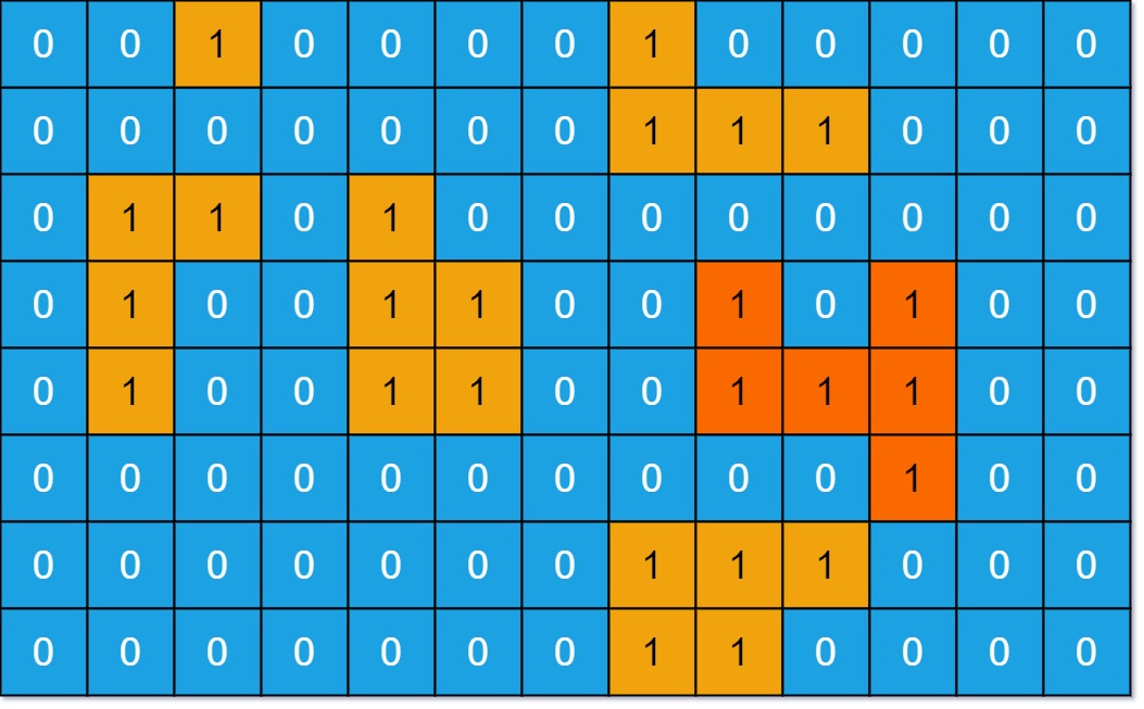
Input: grid = [[0,0,1,0,0,0,0,1,0,0,0,0,0],[0,0,0,0,0,0,0,1,1,1,0,0,0],[0,1,1,0,1,0,0,0,0,0,0,0,0],[0,1,0,0,1,1,0,0,1,0,1,0,0],[0,1,0,0,1,1,0,0,1,1,1,0,0],[0,0,0,0,0,0,0,0,0,0,1,0,0],[0,0,0,0,0,0,0,1,1,1,0,0,0],[0,0,0,0,0,0,0,1,1,0,0,0,0]] Output: 6 Explanation: The answer is not 11, because the island must be connected 4-directionally.
Example 2:
Input: grid = [[0,0,0,0,0,0,0,0]] Output: 0
Constraints:
m =grid.length=n =grid[i].length=1 <m, n <= 50=grid[i][j]is either0or1.
※ 2.12.3.1. Constraints and Edge Cases
- this is flood-fill but different thing that we’re accumulating here (max area)
※ 2.12.3.2. My Solution (Code)
※ 2.12.3.2.1. v1: correct, working iterative BFS flood fill
1: from collections import deque 2: 3: class Solution: 4: │ def maxAreaOfIsland(self, grid: List[List[int]]) -> int: 5: │ │ if not grid or not grid[0]: 6: │ │ │ return 0 7: │ │ │ 8: │ │ area = 0 9: │ │ 10: │ │ ROWS, COLS = len(grid), len(grid[0]) 11: │ │ directions = [(0, 1), (0, -1), (1, 0), (-1, 0)] 12: │ │ 13: │ │ for r in range(ROWS): 14: │ │ │ for c in range(COLS): 15: │ │ │ │ if grid[r][c] == 1: 16: │ │ │ │ │ curr_area = 0 17: │ │ │ │ │ # use as root and carry on: 18: │ │ │ │ │ queue = deque([(r, c)]) 19: │ │ │ │ │ grid[r][c] = 0 20: │ │ │ │ │ curr_area += 1 21: │ │ │ │ │ while queue: 22: │ │ │ │ │ │ r, c = queue.popleft() 23: │ │ │ │ │ │ valid_children = ((r + dr, c + dc) for dr, dc in directions if 0 <= r + dr < ROWS and 0 <= c + dc < COLS and grid[r + dr][c + dc] == 1 ) 24: │ │ │ │ │ │ 25: │ │ │ │ │ │ for child_row, child_col in valid_children: 26: │ │ │ │ │ │ │ # update accumulators (curr_area, visited) 27: │ │ │ │ │ │ │ grid[child_row][child_col] = 0 28: │ │ │ │ │ │ │ curr_area += 1 29: │ │ │ │ │ │ │ 30: │ │ │ │ │ │ │ # enqueue 31: │ │ │ │ │ │ │ queue.append((child_row, child_col)) 32: │ │ │ │ │ │ │ 33: │ │ │ │ │ area = max(area, curr_area) 34: │ │ │ │ │ 35: │ │ return area
- Time:
- Each cell is visited at most once.
- For each land cell, \(O(1)\) per neighbor.
- Total: \(O(m*n)\) (where \(m\) = rows, \(n\) = cols)
- Space:
- The queue holds \(O(\text{area of one island})\) cells at worst, so up to \(O(m*n)\) if the whole grid is one island (rare).
- No explicit visited array; grid is marked in-place.
※ 2.12.3.2.2. alternative v2 DFS:
1: class Solution: 2: │ def maxAreaOfIsland(self, grid: List[List[int]]) -> int: 3: │ │ max_area = 0 4: │ │ rows, cols = len(grid), len(grid[0]) 5: │ │ for r in range(rows): 6: │ │ │ for c in range(cols): 7: │ │ │ │ if grid[r][c] == 1: 8: │ │ │ │ │ stack = [(r, c)] 9: │ │ │ │ │ grid[r][c] = 0 10: │ │ │ │ │ area = 1 11: │ │ │ │ │ while stack: 12: │ │ │ │ │ │ cr, cc = stack.pop() 13: │ │ │ │ │ │ for dr, dc in [(-1,0),(1,0),(0,-1),(0,1)]: 14: │ │ │ │ │ │ │ nr, nc = cr+dr, cc+dc 15: │ │ │ │ │ │ │ if 0 <= nr < rows and 0 <= nc < cols and grid[nr][nc] == 1: 16: │ │ │ │ │ │ │ │ grid[nr][nc] = 0 17: │ │ │ │ │ │ │ │ stack.append((nr, nc)) 18: │ │ │ │ │ │ │ │ area += 1 19: │ │ │ │ │ max_area = max(max_area, area) 20: │ │ return max_area
Recursive DFS will work for these constraints (generous)
1: def dfs(r, c): 2: │ if not (0 <= r < rows and 0 <= c < cols and grid[r][c] == 1): 3: │ │ return 0 4: │ grid[r][c] = 0 5: │ return 1 + sum(dfs(r+dr, c+dc) for dr, dc in directions)
※ 2.12.3.2.3. alternative v3 Union Find
Union Find (Disjoint Set):
Build a parent-pointer mapping for every land cell and union adjacent lands; then, for each root, count how many members its island has. It’s not natural for “area as you traverse”, but possible. Useful for more dynamic problems or when many operations and queries are needed.
It’s more complex of an implementation.
1: class DSU: 2: │ def __init__(self): 3: │ │ self.parent = {} 4: │ │ self.size = {} 5: │ def find(self, x): 6: │ │ if self.parent[x] != x: 7: │ │ │ self.parent[x] = self.find(self.parent[x]) 8: │ │ return self.parent[x] 9: │ def union(self, x, y): 10: │ │ xr, yr = self.find(x), self.find(y) 11: │ │ if xr != yr: 12: │ │ │ self.parent[xr] = yr 13: │ │ │ self.size[yr] += self.size[xr] 14: │ def add(self, x): 15: │ │ if x not in self.parent: 16: │ │ │ self.parent[x] = x 17: │ │ │ self.size[x] = 1 18: │ │ │ 19: # Inside solution, union adjacent '1' cells as you read the grid, 20: # then return max(dsu.size.values()) as the answer if any, else 0.
※ 2.12.3.3. My Approach/Explanation
I’ve done an iterative BFS flood-fill for this, accumulating the max area.
※ 2.12.3.4. My Learnings/Questions
- I am speed.
※ 2.12.3.5. [Optional] Additional Context
I was really fast at implementing this correctly!
※ 2.12.3.6. Retro
-
- Viewed it as running traversals on subgraphs, keeping a local count. Similar to island counting but keeping a local count instead.
- for style, the genexp is harder to read, probably shouldn’t do it.
※ 2.12.4. [82] Clone Graph (133) BFS undirected_graph almost
Given a reference of a node in a connected undirected graph.
Return a deep copy (clone) of the graph.
Each node in the graph contains a value (int) and a list
(List[Node]) of its neighbors.
class Node {
public int val;
public List<Node> neighbors;
}
Test case format:
For simplicity, each node’s value is the same as the node’s index
(1-indexed). For example, the first node with val = 1=, the second
node with val = 2=, and so on. The graph is represented in the test
case using an adjacency list.
An adjacency list is a collection of unordered lists used to represent a finite graph. Each list describes the set of neighbors of a node in the graph.
The given node will always be the first node with val = 1. You must
return the copy of the given node as a reference to the cloned graph.
Example 1:
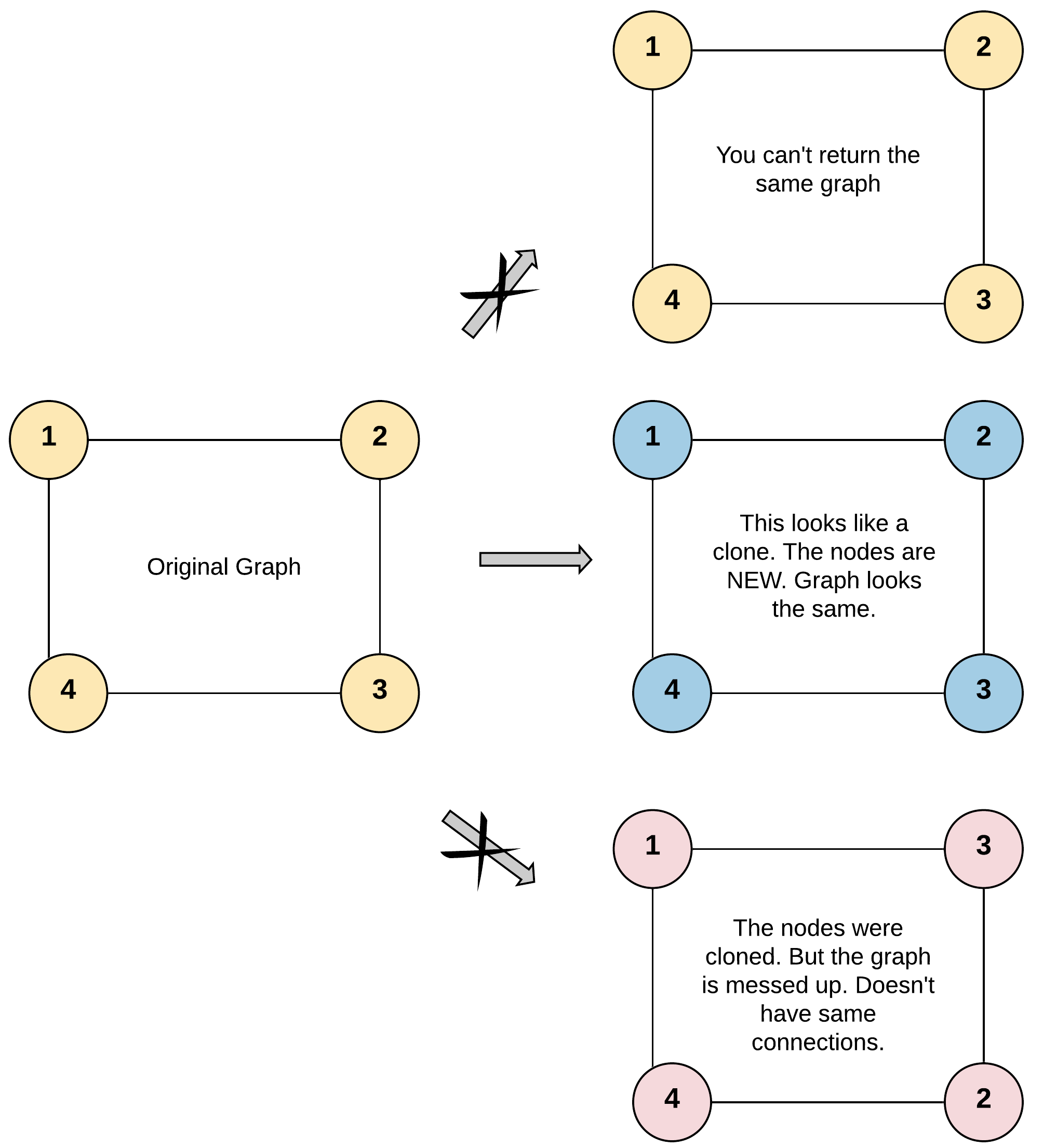
Input: adjList = [[2,4],[1,3],[2,4],[1,3]] Output: [[2,4],[1,3],[2,4],[1,3]] Explanation: There are 4 nodes in the graph. 1st node (val = 1)'s neighbors are 2nd node (val = 2) and 4th node (val = 4). 2nd node (val = 2)'s neighbors are 1st node (val = 1) and 3rd node (val = 3). 3rd node (val = 3)'s neighbors are 2nd node (val = 2) and 4th node (val = 4). 4th node (val = 4)'s neighbors are 1st node (val = 1) and 3rd node (val = 3).
Example 2:
Input: adjList = [[]] Output: [[]] Explanation: Note that the input contains one empty list. The graph consists of only one node with val = 1 and it does not have any neighbors.
Example 3:
Input: adjList = [] Output: [] Explanation: This an empty graph, it does not have any nodes.
Constraints:
- The number of nodes in the graph is in the range
[0, 100]. 1 <Node.val <= 100=Node.valis unique for each node.- There are no repeated edges and no self-loops in the graph.
- The Graph is connected and all nodes can be visited starting from the given node.
※ 2.12.4.1. Constraints and Edge Cases
- rmb the values are 1-idxed but doesn’t matter because we’re just copying it from the old versions.
※ 2.12.4.2. My Solution (Code)
※ 2.12.4.2.1. wrong v0: alright structure for BFS, inaccuracies
This seems to have an alright structure but with some bugs.
1: """ 2: # Definition for a Node. 3: class Node: 4: │ def __init__(self, val = 0, neighbors = None): 5: │ self.val = val 6: │ self.neighbors = neighbors if neighbors is not None else [] 7: """ 8: 9: from collections import deque 10: 11: from typing import Optional 12: class Solution: 13: │ def cloneGraph(self, node: Optional['Node']) -> Optional['Node']: 14: │ │ 15: │ │ if not node: 16: │ │ │ return None 17: │ │ │ 18: │ │ head = node 19: │ │ 20: │ │ old_to_new = {} 21: │ │ visited = set() 22: │ │ 23: │ │ # traverse the adj list: 24: │ │ # queue will only have the old nodes there 25: │ │ queue = deque([node]) 26: │ │ 27: │ │ while queue: 28: │ │ │ node = queue.popleft() 29: │ │ │ 30: │ │ │ if node in old_to_new: 31: │ │ │ │ new = old_to_new[node] 32: │ │ │ else: 33: │ │ │ │ new = Node(val=node.val) 34: │ │ │ │ old_to_new[node] = new 35: │ │ │ │ 36: │ │ │ for n in node.neighbors: 37: │ │ │ │ edge = (node.val, n.val) 38: │ │ │ │ 39: │ │ │ │ if edge in visited: 40: │ │ │ │ │ continue 41: │ │ │ │ else: 42: │ │ │ │ │ visited.add(edge) 43: │ │ │ │ │ if n in old_to_new: 44: │ │ │ │ │ │ new_n = old_to_new[n] 45: │ │ │ │ │ else: 46: │ │ │ │ │ │ new_n = Node(val=n.val) 47: │ │ │ │ │ │ 48: │ │ │ │ │ │ 49: │ │ │ │ │ old_to_new[node].neighbors.append(new_n) 50: │ │ │ │ │ 51: │ │ │ │ │ queue.append(n) 52: │ │ │ │ │ 53: │ │ return old_to_new[head]
- Problems:
MAIN PROBLEM:
not all new nodes are saved in the mapping, that’s why I had an error
- Some improvements:
- You append queue.append(n) no matter what. In a correct BFS, you should only append a node for further traversal if you haven’t already cloned/visited it.
Inefficiency (multiple times in queue, extra work on visited edges)
With this edge-based check you may be visiting more than necessary.
※ 2.12.4.2.2. working v1: fixed minor bug:
by just adding the one that I missed, the correctness bug will be fixed:
1: """ 2: # Definition for a Node. 3: class Node: 4: │ def __init__(self, val = 0, neighbors = None): 5: │ self.val = val 6: │ self.neighbors = neighbors if neighbors is not None else [] 7: """ 8: 9: from collections import deque 10: 11: from typing import Optional 12: class Solution: 13: │ def cloneGraph(self, node: Optional['Node']) -> Optional['Node']: 14: │ │ 15: │ │ if not node: 16: │ │ │ return None 17: │ │ │ 18: │ │ head = node 19: │ │ 20: │ │ old_to_new = {} 21: │ │ visited = set() 22: │ │ 23: │ │ # traverse the adj list: 24: │ │ # queue will only have the old nodes there 25: │ │ queue = deque([node]) 26: │ │ 27: │ │ while queue: 28: │ │ │ node = queue.popleft() 29: │ │ │ 30: │ │ │ if node in old_to_new: 31: │ │ │ │ new = old_to_new[node] 32: │ │ │ else: 33: │ │ │ │ new = Node(val=node.val) 34: │ │ │ │ old_to_new[node] = new 35: │ │ │ │ 36: │ │ │ for n in node.neighbors: 37: │ │ │ │ edge = (node.val, n.val) 38: │ │ │ │ 39: │ │ │ │ if edge in visited: 40: │ │ │ │ │ continue 41: │ │ │ │ else: 42: │ │ │ │ │ visited.add(edge) 43: │ │ │ │ │ if n in old_to_new: 44: │ │ │ │ │ │ new_n = old_to_new[n] 45: │ │ │ │ │ else: 46: │ │ │ │ │ │ new_n = Node(val=n.val) 47: │ │ │ │ │ │ old_to_new[n] = new_n 48: │ │ │ │ │ │ 49: │ │ │ │ │ old_to_new[node].neighbors.append(new_n) 50: │ │ │ │ │ 51: │ │ │ │ │ queue.append(n) 52: │ │ │ │ │ 53: │ │ return old_to_new[head]
※ 2.12.4.2.3. clean, optimal solution (BFS):
- Key Points:
- Track visited nodes by keys in
old_to_new. - Only add to queue if not in mapping.
- Always map the original node to exactly one clone.
- No need for an explicit visited set when using a mapping.
- Track visited nodes by keys in
1: from collections import deque 2: from typing import Optional 3: 4: class Solution: 5: │ def cloneGraph(self, node: Optional['Node']) -> Optional['Node']: 6: │ │ if not node: 7: │ │ │ return None 8: │ │ │ 9: │ │ old_to_new = {} 10: │ │ queue = deque([node]) 11: │ │ old_to_new[node] = Node(val=node.val) 12: │ │ 13: │ │ while queue: 14: │ │ │ cur = queue.popleft() 15: │ │ │ for neighbor in cur.neighbors: 16: │ │ │ │ if neighbor not in old_to_new: 17: │ │ │ │ │ old_to_new[neighbor] = Node(val=neighbor.val) 18: │ │ │ │ │ queue.append(neighbor) 19: │ │ │ │ old_to_new[cur].neighbors.append(old_to_new[neighbor]) 20: │ │ │ │ 21: │ │ return old_to_new[node]
- Let \(N\) = number of nodes; \(E\) = number of edges.
- Time:
- Every node and every edge is visited once (BFS).
- For each node, you iterate over all its neighbors.
- Total: \(O(N+E)\)
- Space:
old_to_newmapping: \(O(N)\)- queue: \(O(N)\) at worst (all nodes enqueued)
- Output: \(O(N+E)\) (if output is counted in space)
- No actual “visited set” is needed beyond the mapping.
- Time:
※ 2.12.4.2.4. clean, optimal Recursive DFS solution
1: class Solution: 2: │ def cloneGraph(self, node: 'Node') -> 'Node': 3: │ │ if not node: 4: │ │ │ return None 5: │ │ old_to_new = {} 6: │ │ def dfs(n): 7: │ │ │ if n in old_to_new: 8: │ │ │ │ return old_to_new[n] 9: │ │ │ copy = Node(n.val) 10: │ │ │ old_to_new[n] = copy 11: │ │ │ for nei in n.neighbors: 12: │ │ │ │ copy.neighbors.append(dfs(nei)) 13: │ │ │ return copy 14: │ │ return dfs(node)
※ 2.12.4.3. My Approach/Explanation
My intent was to use undirected graphs as bidirectional edges, and then to track the edges that have already been navigated.
※ 2.12.4.4. My Learnings/Questions
- Graph cloning just needs to do instance check for nodes, not edges.
- The right way is to track instance identity, not just value.
Use of
visitedmay not apply for the general case:You’re tracking visited edges as
(node.val, n.val), which is not what’s required for graph cloning.This will not work if two different nodes have the same value.
Graph traversal should be node-based, not edge-based.
This can lead to duplicated nodes or missed edges in your clone, especially if val is not unique.
QQ: in which case, can i just keep an edge = (n1, n2) where n1 and n2 are two different nodes? Can I just keep an edge = (n1, n2) where n1 and n2 are two different nodes?
You could track visited edges this way if you were, say, exploring for edge-based properties (like cycle detection), but for graph cloning you only need to clone nodes and link them.
The edge-tracking method is unnecessary complication and can go wrong if you confuse node identity (different node objects, or nodes with same values).
The right way is to use the node’s object identity as the mapping key, as you did in oldtonew.
In which case should I use edge-based visited tracking?
Rare in “clone” scenarios. You use it more for algorithms needing explicit edge visit history (e.g., Eulerian path/circuit, multi-graph algorithms, or truly directed edges you care about visited order).
※ 2.12.4.5. Retros
Just need to do a traversal while keeping some aux nodes and adding the neighbor relationships correctly
Graph traversal is about traversing the nodes, not the edges. Things are usually Hamiltonian in nature.
※ 2.12.5. [83] Walls and Gates (??) multi_source_BFS
> [leetcode description]
Walls and Gates
You are given an m x n grid rooms initialized with these three possible values:
- -1
- A wall or an obstacle.
- 0
- A gate.
- INF
- An empty room. (We use the value ~2147483647~—that is, ~231-1~—to represent INF.)
Fill each empty room with the number of steps to its nearest gate. If it is impossible to reach a gate, keep it as INF.
You may move up, down, left, or right (not diagonally).
You must fill the grid in place (do not return anything).
Example:
Input: rooms = [ [2147483647, -1, 0, 2147483647], [2147483647, 2147483647, 2147483647, -1], [2147483647, -1, 2147483647, -1], [0, -1, 2147483647, 2147483647] ] Output (after function call, 'rooms' is modified to): [ [3, -1, 0, 1], [2, 2, 1, -1], [1, -1, 2, -1], [0, -1, 3, 4] ]
Constraints:
m == rooms.lengthn == rooms[i].length1 <= m, n <= 250rooms[i][j]is -1, 0, or 2147483647 (INF)
Note: A typical solution uses multi-source BFS starting from all gates (cells with value 0) at once.
> [neetcode description]
Islands and Treasure
You are given a \( m \times n \) 2D grid initialized with these three possible values:
- -1 - A water cell that can not be traversed.
- 0 - A treasure chest.
- INF - A land cell that can be traversed. We use the integer `231 - 1 = 2147483647` to represent INF.
Fill each land cell with the distance to its nearest treasure chest. If a land cell cannot reach a treasure chest then the value should remain INF.
Assume the grid can only be traversed up, down, left, or right.
Modify the grid in-place.
Example 1:
Input: [ [2147483647, -1, 0, 2147483647], [2147483647, 2147483647, 2147483647, -1], [2147483647, -1, 2147483647, -1], [0, -1, 2147483647, 2147483647] ] Output: [ [3, -1, 0, 1], [2, 2, 1, -1], [1, -1, 2, -1], [0, -1, 3, 4] ]
Example 2:
Input: [ [0, -1], [2147483647, 2147483647] ] Output: [ [0, -1], [1, 2] ]
Constraints:
m == grid.lengthn == grid[i].length1 <= m, n <= 100grid[i][j]is one of {-1, 0, 2147483647}
Hints & Complexity Guidance
Recommended Time & Space Complexity
You should aim for a solution with O(m * n) time and O(m * n) space, where m is the number of rows and n is the number of columns in the given grid.
Hint 1:
A brute force solution would be to iterate on each land cell and run a BFS from that cell to find the nearest treasure chest. This would be an O((m * n)^2) solution. Can you think of a better way? Sometimes it is not optimal to go from source to destination.
Hint 2: We can see that instead of going from every cell to find the nearest treasure chest, we can do it in reverse. We can just do a BFS from all the treasure chests in grid and just explore all possible paths from those chests. Why? Because in this approach, the treasure chests self-mark the cells level by level and the level number will be the distance from that cell to a treasure chest. We don’t revisit a cell. This approach is called Multi-Source BFS. How would you implement it?
Hint 3:
We insert all the cells (row, col) that represent the treasure chests into the queue. Then, we process the cells level by level, handling all the current cells in the queue at once. For each cell, we mark it as visited and store the current level value as the distance at that cell. We then try to add the neighboring cells (adjacent cells) to the queue, but only if they have not been visited and are land cells.
※ 2.12.5.1. Constraints and Edge Cases
- empty grid early return
※ 2.12.5.2. My Solution (Code)
※ 2.12.5.2.1. [failed] V1: flood fill from multiple sources, one by one
This is a little inconvenient to do because I can’t access it directly on leetcode.
My intent is to just do BFS flood fill from all treasures outwards.
I should be relaxing the estimates and only if I relax the estimates, the node should be added back into the queue.
1: from collections import deque 2: 3: class Solution: 4: │ def islandsAndTreasure(self, grid: List[List[int]]) -> None: 5: │ │ ROWS, COLS = len(grid), len(grid[0]) 6: │ │ DIRS = [(0, -1), (0, 1), (1, 0), (-1, 0)] 7: │ │ 8: │ │ def bfs(r, c): 9: │ │ │ queue = deque([((r,c), 0)]) 10: │ │ │ while queue: 11: │ │ │ │ # get the layer: 12: │ │ │ │ for _ in range(len(queue)): 13: │ │ │ │ │ coord, hop = queue.popleft() 14: │ │ │ │ │ row,col = coord 15: │ │ │ │ │ node = grid[row][col] 16: │ │ │ │ │ if node == -1: 17: │ │ │ │ │ │ continue 18: │ │ │ │ │ else: 19: │ │ │ │ │ │ curr = grid[row][col] 20: │ │ │ │ │ │ if hop < curr: 21: │ │ │ │ │ │ │ grid[row][col] = hop 22: │ │ │ │ │ │ │ queue.extend[((rlw + dr, col + dc), hop + 1) for dr, dc in DIRS if 0 <= row + dr < ROWS and 0 <= col + dc < COLS and grid[row + dr][col + dc] > 0] 23: │ │ │ return 24: │ │ │ 25: │ │ for r in range(ROWS): 26: │ │ │ for c in range(COLS): 27: │ │ │ │ # find treasure chest: 28: │ │ │ │ if grid[r][c] == 0: 29: │ │ │ │ │ bfs(r, c) 30: │ │ return
this solution is flawed because:
- Redundant work:
- You’re running BFS from every gate, and each BFS may repeat efforts of previous ones (updating the same room multiple times if it is in reach of multiple gates).
- Inefficient visitation:
- There’s no tracking of whether a cell has already been set to its optimal value by a different, closer BFS. (You do check hop < curr before updating, but you still may hit the same cell from multiple sources, and add the same cell to the queue more than once per gate.)
- Minor typo:
- In
queue.extend[((rlw + dr, col + dc), hop + 1)...]should bequeue.extend([...]), andrlwshould berow.
- In
- Inefficient time complexity:
- Because each BFS can touch nearly all other cells, worst-case time is O(KNM) where K = number of gates.
※ 2.12.5.2.2. [correct] Multi-source BFS simultaneously
1: from collections import deque 2: 3: def wallsAndGates(rooms): 4: │ if not rooms: 5: │ │ return 6: │ ROWS, COLS = len(rooms), len(rooms[0]) 7: │ queue = deque() 8: │ INF = 2147483647 9: │ 10: │ # Add all gates to queue at distance 0 11: │ for r in range(ROWS): 12: │ │ for c in range(COLS): 13: │ │ │ if rooms[r][c] == 0: 14: │ │ │ │ queue.append((r, c)) 15: │ │ │ │ 16: │ directions = [(-1,0),(1,0),(0,-1),(0,1)] 17: │ 18: │ while queue: 19: │ │ r, c = queue.popleft() 20: │ │ for dr, dc in directions: 21: │ │ │ nr, nc = r+dr, c+dc 22: │ │ │ if 0 <= nr < ROWS and 0 <= nc < COLS and rooms[nr][nc] == INF: 23: │ │ │ │ rooms[nr][nc] = rooms[r][c] + 1 24: │ │ │ │ queue.append((nr, nc)) 25:
Shifted over to the neetcode version:
1: from collections import deque 2: 3: class Solution: 4: │ def islandsAndTreasure(self, grid: List[List[int]]) -> None: 5: │ │ if not grid: 6: │ │ │ return 7: │ │ │ 8: │ │ queue = deque() 9: │ │ ROWS, COLS = len(grid), len(grid[0]) 10: │ │ DIRS = [(0, -1), (0, 1), (1, 0), (-1, 0)] 11: │ │ INF = 2147483647 12: │ │ 13: │ │ # 1: add all gates to queue at distance 0 (multiple source, simultaneous) 14: │ │ for r in range(ROWS): 15: │ │ │ for c in range(COLS): 16: │ │ │ │ # is treasure: 17: │ │ │ │ if grid[r][c] == 0: 18: │ │ │ │ │ queue.append((r, c)) 19: │ │ │ │ │ 20: │ │ while queue: 21: │ │ │ r, c = queue.popleft() 22: │ │ │ candidates = ((r + dr, c + dc) for dr, dc in DIRS if (0 <= r + dr < ROWS) and (0 <= c + dc < COLS) and grid[r + dr][c + dc] == INF) 23: │ │ │ for row, col in candidates: 24: │ │ │ │ grid[row][col] = grid[r][c] + 1 25: │ │ │ │ queue.append((row, col))
NOTE:
Only updates INF cells (unvisited rooms).
As soon as a room is filled, we do not revisit it, since the first traversal is always the shortest, due to BFS’s layer-by-layer nature.
※ 2.12.5.3. My Approach/Explanation
Looks like the optimal solution involves multi-source BFS simultaneously.
※ 2.12.5.4. My Learnings/Questions
key intuition: This is a classic example of “frontier grows out from all sources at once” (multi-source BFS, or ripple fill) being much more efficient than searching from every destination independently.
BFS only works here because the move-cost is always 1, else we would have had to use Dijkstra.
Instead of BFS from every gate individually, do multi-source BFS:
- Enqueue all gates at once as starting points.
- From each gate, expand level-by-level; when a room is visited for the first time (from its nearest gate), assign its distance and do not revisit.
- multi-source BFS is not that different from single-source DFS, it’s just more things to init the queue with.
- alternatives:
- Dijkstra’s algorithm:
Would be needed if cell-to-cell costs were not all 1. Since every movement is cost-1, BFS suffices. Here’s a problem variation for it:
Problem Variation: Weighted Walls and Gates- Suppose each move (to a neighbor cell) has a cost (not always 1).
- Each cell may have an associated cost to enter it (NOT just 0 or 1).
- Find the minimal cost to reach the nearest gate (cell with value 0) for every empty cell (INF).
- Rules
- You may move up/down/left/right.
- Walls (value -1) are impassable.
- Gates (value 0) are your sources.
- Every cell rooms[r][c] > 0 has a cost: you must pay this cost to step INTO the cell from its neighbor.
You must fill each empty cell with the minimum total cost to reach a gate. If a gate is unreachable, leave as INF (2147483647). Sample Input
rooms = [ [2147483647, -1, 0, 2147483647], [2, 2, 1, -1], [2147483647, -1, 3, -1], [0, -1, 1, 1] ]
Here, walking “into” cell (1,0) costs 2, into (1,1) costs 2, into (2,2) costs 3, etc.
So the solution to this would be to use Dijkstra’s Algorithm:
Show/Hide Python Code1: import heapq 2: 3: def wallsAndGatesWeighted(rooms): 4: │ if not rooms or not rooms[0]: 5: │ │ return 6: │ INF = 2147483647 7: │ m, n = len(rooms), len(rooms[0]) 8: │ heap = [] 9: │ # Initialize: all gates at cost 0 10: │ for r in range(m): 11: │ │ for c in range(n): 12: │ │ │ if rooms[r][c] == 0: 13: │ │ │ │ heapq.heappush(heap, (0, r, c)) 14: │ directions = [(-1,0),(1,0),(0,-1),(0,1)] 15: │ visited = set() # For potential cycles 16: │ 17: │ while heap: 18: │ │ curr_cost, r, c = heapq.heappop(heap) 19: │ │ if (r, c) in visited: 20: │ │ │ continue 21: │ │ visited.add((r, c)) 22: │ │ for dr, dc in directions: 23: │ │ │ nr, nc = r + dr, c + dc 24: │ │ │ # Standard bounds & wall checks 25: │ │ │ if ( 26: │ │ │ │ 0 <= nr < m and 0 <= nc < n and 27: │ │ │ │ rooms[nr][nc] != -1 and (nr, nc) not in visited 28: │ │ │ ): 29: │ │ │ │ # If the neighbor is not a gate (don't reassign a 0) 30: │ │ │ │ enter_cost = rooms[nr][nc] if rooms[nr][nc] not in (INF, 0) else 1 31: │ │ │ │ new_cost = curr_cost + enter_cost 32: │ │ │ │ # Only update if found a better (lower) cost 33: │ │ │ │ if rooms[nr][nc] == INF or (rooms[nr][nc] > 0 and new_cost < rooms[nr][nc]): 34: │ │ │ │ │ rooms[nr][nc] = new_cost 35: │ │ │ │ │ heapq.heappush(heap, (new_cost, nr, nc)) 36: │ │ │ │ │ 37: # Example Usage: 38: rooms = [ 39: │ [2147483647, -1, 0, 2147483647], 40: │ [2, 2, 1, -1], 41: │ [2147483647, -1, 3, -1], 42: │ [0, -1, 1, 1] 43: ] 44: wallsAndGatesWeighted(rooms) 45: for row in rooms: 46: │ print(row) 47:
- Suppose each move (to a neighbor cell) has a cost (not always 1).
- DFS:
- Would not guarantee minimal steps for graphs with cycles/ambiguous paths; not appropriate here.
- Dijkstra’s algorithm:
※ 2.12.5.5. Retros
Nothing fancy here, just need to do multiple traversals, each source being a treasure chest.
Simultaneously we can run the multi source BFS, we could have loaded the “height” of the parent within the children but not really necessary here.
If it was differently weighted (and positive), I’d have to run Dijkstra’s with cycle checking.
※ 2.12.6. [84] Rotting Oranges (994) multi_source_BFS simulated_time_frontier
You are given an m x n grid where each cell can have one of three
values:
0representing an empty cell,1representing a fresh orange, or2representing a rotten orange.
Every minute, any fresh orange that is 4-directionally adjacent to a rotten orange becomes rotten.
Return the minimum number of minutes that must elapse until no cell has
a fresh orange. If this is impossible, return -1.
Example 1:
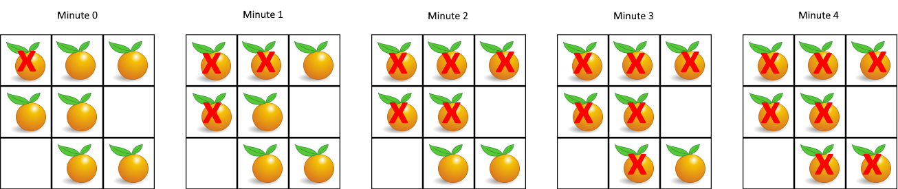
Input: grid = [[2,1,1],[1,1,0],[0,1,1]] Output: 4
Example 2:
Input: grid = [[2,1,1],[0,1,1],[1,0,1]] Output: -1 Explanation: The orange in the bottom left corner (row 2, column 0) is never rotten, because rotting only happens 4-directionally.
Example 3:
Input: grid = [[0,2]] Output: 0 Explanation: Since there are already no fresh oranges at minute 0, the answer is just 0.
Constraints:
m =grid.length=n =grid[i].length=1 <m, n <= 10=grid[i][j]is0,1, or2.
※ 2.12.6.1. Constraints and Edge Cases
- Careful on return values:
- the return val for empty case is 0
- the return val for impossible case is -1
※ 2.12.6.2. My Solution (Code)
※ 2.12.6.2.1. [correct] v0: multi-source BFS
1: from collections import deque 2: 3: class Solution: 4: │ def orangesRotting(self, grid: List[List[int]]) -> int: 5: │ │ if not len(grid) or not len(grid[0]): 6: │ │ │ return 0 7: │ │ │ 8: │ │ ROWS, COLS = len(grid), len(grid[0]) 9: │ │ DIRS = [(0, -1), (0, 1), (1, 0), (-1, 0)] 10: │ │ queue = deque() 11: │ │ 12: │ │ max_t = 0 13: │ │ 14: │ │ # add all rotten sources first: 15: │ │ for r in range(ROWS): 16: │ │ │ for c in range(COLS): 17: │ │ │ │ # if is rotten, start tracking: 18: │ │ │ │ if grid[r][c] == 2: 19: │ │ │ │ │ queue.append(((r, c), 0)) 20: │ │ │ │ │ 21: │ │ while queue: 22: │ │ │ coord, t = queue.popleft() 23: │ │ │ r, c = coord 24: │ │ │ candidates = (((r + dr, c + dc), t + 1) for dr, dc in DIRS if (0 <= r + dr < ROWS) and (0 <= c + dc < COLS) and grid[r + dr][c + dc] == 1) 25: │ │ │ for (row, col), time in candidates: 26: │ │ │ │ max_t = max(max_t, time) 27: │ │ │ │ queue.append(((row, col), time)) 28: │ │ │ │ grid[row][col] = 2 29: │ │ │ │ 30: │ │ return -1 if any(grid[r][c] == 1 for r in range(ROWS) for c in range(COLS)) else max_t
- Complexity Analysis
- Time:
- Each cell is processed at most once. For an
m×ngrid: - \(O(mn)\)
- Each cell is processed at most once. For an
- Space:
- The queue can grow to contain at most \(O(mn)\) cells (in pathological cases).
- So \(O(mn)\) space (input space not counted; queue is the main extra space).
- Time:
※ 2.12.6.2.2. [correct] v0 Cleaned: Multi-Source BFS
1: from collections import deque 2: class Solution: 3: │ def orangesRotting(self, grid: List[List[int]]) -> int: 4: │ │ ROWS, COLS = len(grid), len(grid[0]) 5: │ │ queue = deque() 6: │ │ fresh = 0 7: │ │ for r in range(ROWS): 8: │ │ │ for c in range(COLS): 9: │ │ │ │ if grid[r][c] == 2: 10: │ │ │ │ │ queue.append((r, c, 0)) 11: │ │ │ │ elif grid[r][c] == 1: 12: │ │ │ │ │ fresh += 1 13: │ │ time = 0 14: │ │ while queue: 15: │ │ │ r, c, t = queue.popleft() 16: │ │ │ for dr, dc in [(-1,0),(1,0),(0,-1),(0,1)]: 17: │ │ │ │ nr, nc = r+dr, c+dc 18: │ │ │ │ if 0 <= nr < ROWS and 0 <= nc < COLS and grid[nr][nc] == 1: 19: │ │ │ │ │ grid[nr][nc] = 2 20: │ │ │ │ │ fresh -= 1 21: │ │ │ │ │ queue.append((nr, nc, t+1)) 22: │ │ │ │ │ time = t+1 23: │ │ return -1 if fresh > 0 else time
※ 2.12.6.3. My Approach/Explanation
Once again it’s a multi-source BFS that we’re doing, we just need to track the max hops to get the max time.
※ 2.12.6.4. My Learnings/Questions
- Intuition:
- Any scenario where you want “minute by minute” spread from multiple origins, use Multi-source BFS.
- For minimal steps or “fill” across a grid, BFS is canonically optimal.
- The queue acts as the “simulated time frontier.”
- pythonic:
we could use listcomps for the variable inits:
Show/Hide Python Code1: queue = deque([(r, c, 0) for r in range(ROWS) for c in range(COLS) if grid[r][c] == 2]) 2: fresh = sum(grid[r][c] == 1 for r in range(ROWS) for c in range(COLS))
TRICK: Optimisation: avoiding the last scan for remaining fresh oranges:
To avoid scanning the grid at the end, you could count fresh at the start, decrement as you rot, and finish as soon as
fresh =0=, but your version is reasonable for this grid size.
※ 2.12.6.5. Retros
This is a time simulation using flood-fill. We need to keep track of time, so we keep the time that the orange rots (by using it’s parent’s time) along with the traversal.
The aux counter for fresh is a nifty trick that helps us avoid another scan of the grid to check if all of them are rotten or not.
※ 2.12.7. [85] ⭐️ Pacific Atlantic Water Flow (417) complement_approach flood_fill simulation border_to_center inverse_requirements reachability
There is an m x n rectangular island that borders both the Pacific
Ocean and Atlantic Ocean. The Pacific Ocean touches the island’s
left and top edges, and the Atlantic Ocean touches the island’s right
and bottom edges.
The island is partitioned into a grid of square cells. You are given an
m x n integer matrix heights where heights[r][c] represents the
height above sea level of the cell at coordinate (r, c).
The island receives a lot of rain, and the rain water can flow to neighboring cells directly north, south, east, and west if the neighboring cell’s height is less than or equal to the current cell’s height. Water can flow from any cell adjacent to an ocean into the ocean.
Return a 2D list of grid coordinates result where
result[i] = [r=_{=i}=, c=i=]= denotes that rain water can flow
from cell (r=_{=i}=, c=i=)= to both the Pacific and Atlantic
oceans.
Example 1:
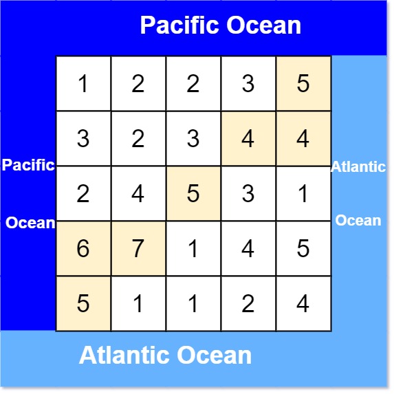
Input: heights = [[1,2,2,3,5],[3,2,3,4,4],[2,4,5,3,1],[6,7,1,4,5],[5,1,1,2,4]]
Output: [[0,4],[1,3],[1,4],[2,2],[3,0],[3,1],[4,0]]
Explanation: The following cells can flow to the Pacific and Atlantic oceans, as shown below:
[0,4]: [0,4] -> Pacific Ocean
[0,4] -> Atlantic Ocean
[1,3]: [1,3] -> [0,3] -> Pacific Ocean
[1,3] -> [1,4] -> Atlantic Ocean
[1,4]: [1,4] -> [1,3] -> [0,3] -> Pacific Ocean
[1,4] -> Atlantic Ocean
[2,2]: [2,2] -> [1,2] -> [0,2] -> Pacific Ocean
[2,2] -> [2,3] -> [2,4] -> Atlantic Ocean
[3,0]: [3,0] -> Pacific Ocean
[3,0] -> [4,0] -> Atlantic Ocean
[3,1]: [3,1] -> [3,0] -> Pacific Ocean
[3,1] -> [4,1] -> Atlantic Ocean
[4,0]: [4,0] -> Pacific Ocean
[4,0] -> Atlantic Ocean
Note that there are other possible paths for these cells to flow to the Pacific and Atlantic oceans.
Example 2:
Input: heights = [[1]] Output: [[0,0]] Explanation: The water can flow from the only cell to the Pacific and Atlantic oceans.
Constraints:
m =heights.length=n =heights[r].length=1 <m, n <= 200=0 <heights[r][c] <= 10=5
※ 2.12.7.1. Constraints and Edge Cases
<list constraints, input limits, or tricky edge cases here>
※ 2.12.7.2. My Solution (Code)
※ 2.12.7.2.1. [incomplete] v0: abandoned attempt
1: class Solution: 2: │ def pacificAtlantic(self, heights: List[List[int]]) -> List[List[int]]: 3: │ │ if not heights or not heights[0]: 4: │ │ │ return [] 5: │ │ ROWS, COLS = len(heights), len(heights[0]) 6: │ │ PAC_DIR = [(-1, 0), (0, -1)] 7: │ │ ATL_DIR = [(0, 1), (1, 0)] 8: │ │ 9: │ │ # tuple: can flow to pacific, can flow to atlantic 10: │ │ flows = [[(None, None) for col in range(COLS)] for row in range(ROWS) ] 11: │ │ 12: │ │ # mark boundaries for pacific: 13: │ │ for r,c in (row, 0) for row in range(ROWS): 14: │ │ │ flows[r][c] = (True, flows[r][c][1]) 15: │ │ │ 16: │ │ for r,c in (0, col) for col in range(COLS): 17: │ │ │ flows[r][c] = (True, flows[r][c][1]) 18: │ │ │ 19: │ │ # mark boundaries for atlantic: 20: │ │ for r,c in (row, COLS - 1) for row in range(ROWS): 21: │ │ │ flows[r][c] = (flows[r][c][0], True) 22: │ │ │ 23: │ │ for r,c in (ROWS - 1, col) for col in range(COLS): 24: │ │ │ flows[r][c] = (flows[r][c][0], True)
※ 2.12.7.2.2. [correct] v1: dual bfs flood fill in inverse direction to determine reachability
this just completest the previous one
1: from collections import deque 2: 3: class Solution: 4: │ def pacificAtlantic(self, heights: List[List[int]]) -> List[List[int]]: 5: │ │ if not heights or not heights[0]: 6: │ │ │ return [] 7: │ │ │ 8: │ │ ROWS, COLS = len(heights), len(heights[0]) 9: │ │ DIRS = [(-1, 0), (1, 0), (0, 1), (0, -1)] 10: │ │ 11: │ │ pacific_visited = [ [False] * COLS for _ in range(ROWS)] 12: │ │ atlantic_visited = [ [False] * COLS for _ in range(ROWS)] 13: │ │ 14: │ │ def bfs(start_coords, visited): 15: │ │ │ queue = deque(start_coords) 16: │ │ │ while queue: 17: │ │ │ │ r, c = queue.popleft() 18: │ │ │ │ visited[r][c] = True 19: │ │ │ │ reachable = ((r + dr, c + dc) for dr, dc in DIRS if 0 <= r + dr < ROWS and 0 <= c + dc < COLS and not visited[r + dr][c + dc] and heights[r + dr][c + dc] >= heights[r][c]) 20: │ │ │ │ for coord in reachable: 21: │ │ │ │ │ queue.append(coord) 22: │ │ │ │ │ 23: │ │ # run bfs for pacific ocean 24: │ │ pacific_start_coords = [(0, c) for c in range(COLS)] + [(r, 0) for r in range(ROWS)] 25: │ │ bfs(pacific_start_coords, pacific_visited) 26: │ │ # run bfs for atlantic ocean 27: │ │ atlantic_start_coords = [(ROWS - 1, c) for c in range(COLS)] + [(r, COLS - 1) for r in range(ROWS)] 28: │ │ bfs(atlantic_start_coords, atlantic_visited) 29: │ │ 30: │ │ return [(r, c) for r in range(ROWS) for c in range(COLS) if pacific_visited[r][c] and atlantic_visited[r][c]]
※ 2.12.7.2.3. [correct] v2: optimised version of v1
Right off the bat, the marking as visited should be done before enqueing not after. This reduces the extra searching and makes things efficient.
from collections import deque class Solution: │ def pacificAtlantic(self, heights: List[List[int]]) -> List[List[int]]: │ │ # early returns for trivial edge case: │ │ if not heights or not heights[0]: │ │ │ return [] │ │ │ │ │ ROWS, COLS = len(heights), len(heights[0]) │ │ DIRS = [(-1,0), (1,0), (0,-1), (0,1)] │ │ │ │ def bfs(starts): │ │ │ visited = set(starts) │ │ │ queue = deque(starts) │ │ │ while queue: │ │ │ │ r, c = queue.popleft() │ │ │ │ # direct for loop is better than generator then for loop: │ │ │ │ for dr, dc in DIRS: │ │ │ │ │ nr, nc = r + dr, c + dc │ │ │ │ │ # is reachable coordinate: │ │ │ │ │ if ( │ │ │ │ │ │ 0 <= nr < ROWS and │ │ │ │ │ │ 0 <= nc < COLS and │ │ │ │ │ │ (nr, nc) not in visited and │ │ │ │ │ │ heights[nr][nc] >= heights[r][c] │ │ │ │ │ ): │ │ │ │ │ │ # mark as visited before enqueing! │ │ │ │ │ │ visited.add((nr, nc)) │ │ │ │ │ │ queue.append((nr, nc)) │ │ │ return visited │ │ │ │ │ pacific_starts = [(0, c) for c in range(COLS)] + [(r, 0) for r in range(ROWS)] │ │ atlantic_starts = [(ROWS-1, c) for c in range(COLS)] + [(r, COLS-1) for r in range(ROWS)] │ │ │ │ pacific_reach = bfs(pacific_starts) │ │ atlantic_reach = bfs(atlantic_starts) │ │ │ │ return [ [r, c] for r, c in (pacific_reach & atlantic_reach) ]
- Complexity Analysis
- Let \(m\) be number of rows and \(n\) be number of columns.
- Time:
- Each BFS runs in \(O(mn)\) (every cell is processed at most once per ocean).
- Total: O(mn)
- Space:
pacific_reach,atlantic_reach, and their queues can each be up to \(O(mn)\).- Total: O(mn)
※ 2.12.7.3. My Approach/Explanation
I’m thinking of doing a BFS on two queues:
- movement towards atlantic
- movement towards pacific
They just have to be done on a separate set of visited.
The key idea here is that instead of focusing on how the water flows, focus on what is reachable from the edges of the map (from the ocean to the cell)
※ 2.12.7.4. My Learnings/Questions
Intuition:
This problem is classic “reverse reachability” for multiple sources — so multi-source BFS or multi-source DFS are always right.
- TRICK: from all ocean-bordering cells, focus on reachability, instead of doing the water flow simulations, so spread reachability only if a neighbour is higher or equal
- pythonic improvements:
Use set comprehensions: For even more clarity when defining the start cells.
Show/Hide Python Code1: pacific_starts = {(0, c) for c in range(COLS)} | {(r, 0) for r in range(ROWS)} 2: atlantic_starts = {(ROWS-1, c) for c in range(COLS)} | {(r, COLS-1) for r in range(ROWS)} 3: pacific_reach = bfs(pacific_starts) 4: atlantic_reach = bfs(atlantic_starts)
- use sets for visited,
- can use set
- opens up the possibility of doing set intersections which are blazingly fast.
- general micro-optimisations:
- mark as visited before enqueing the node
- direct inline loop and not the generator-then-loop implementation
- mark the start points right away, don’t visit them multiple times
※ 2.12.7.5. [Optional] Additional Context
Good example of a ’complement approach’ / ’inverse requirements’ to finding the trick in the question.
※ 2.12.7.6. Retros
We always need to ask the basic questions first, in this case, knowing that it’s a traversal (literal flood fill)
- what’s the source and what’s the destination? here it’s easier to find out the boundaries as the source
- multisource? two separate parallel runs?
This part is beautiful
Show/Hide Python Code1: │ │ pacific_reach = bfs(pacific_starts) 2: │ │ atlantic_reach = bfs(atlantic_starts) 3: │ │ 4: │ │ return [ [r, c] for r, c in (pacific_reach & atlantic_reach) ]
※ 2.12.8. [86] Surrounded Regions (130) bad_question complement_approach intermediate_marks border_to_center
You are given an m x n matrix board containing letters 'X' and
'O', capture regions that are surrounded:
- Connect: A cell is connected to adjacent cells horizontally or vertically.
- Region: To form a region connect every
'O'cell. - Surround: The region is surrounded with
'X'cells if you can connect the region with'X'cells and none of the region cells are on the edge of theboard.
To capture a surrounded region, replace all =’O’=s with =’X’=s in-place within the original board. You do not need to return anything.
Example 1:
Input: board =
[["X","X","X","X"],["X","O","O","X"],["X","X","O","X"],["X","O","X","X"]]
Output:
[["X","X","X","X"],["X","X","X","X"],["X","X","X","X"],["X","O","X","X"]]
Explanation:
 In the above diagram, the bottom region is not captured because it is on
the edge of the board and cannot be surrounded.
In the above diagram, the bottom region is not captured because it is on
the edge of the board and cannot be surrounded.
Example 2:
Input: board = [["X"]]
Output: [["X"]]
Constraints:
m =board.length=n =board[i].length=1 <m, n <= 200=board[i][j]is'X'or'O'.
※ 2.12.8.1. Constraints and Edge Cases
- careful on the char encodings like here it’s an uppercase
'O'and not a'0'
※ 2.12.8.2. My Solution (Code)
※ 2.12.8.2.1. [wrong] V1: misinterpretation
Though I don’t blame myself for this.
1: from collections import deque 2: class Solution: 3: │ def solve(self, board: List[List[str]]) -> None: 4: │ │ """ 5: │ │ Do not return anything, modify board in-place instead. 6: │ │ """ 7: │ │ if not board or not board[0]: 8: │ │ │ return 9: │ │ │ 10: │ │ ROWS, COLS = len(board), len(board[0]) 11: │ │ DIRS = [(0, 1), (0, -1), (1, 0), (-1, 0)] 12: │ │ 13: │ │ 14: │ │ # it's like a flood fill with multiple candidates and we just need to do the swapping 15: │ │ # doing a BFS 16: │ │ def bfs(starts): 17: │ │ │ queue = deque(starts) 18: │ │ │ while queue: 19: │ │ │ │ r, c = queue.popleft() 20: │ │ │ │ neis = [(r + dr, c + dc) for dr, dc in DIRS 21: │ │ │ │ │ │ if (0 <= r + dr < ROWS ) and (0 <= c + dc < COLS)] 22: │ │ │ │ can_connect = any([board[r][c] == 'X' for r, c in neis]) 23: │ │ │ │ if can_connect: 24: │ │ │ │ │ board[r][c] = 'X' 25: │ │ │ │ │ new_candidates = [(r, c) for r,c in neis if board[r][c] == 'O' and 1 <= r < ROWS - 1 and 1 <= c < COLS - 1] 26: │ │ │ │ │ queue.extend(new_candidates) 27: │ │ │ │ │ 28: │ │ starts = {(row, col) for row in range(1, ROWS - 1) for col in range(1, COLS - 1) if board[row][col] == 'O'}
Seems like what the question means is that we need to identify all those that can’t be surrounded. So we need to flood fill from the edge nodes onwards and mark them are “UNSURROUNDABLE”. The rest can just be converted to “SURROUNDABLE” and changed in place.
※ 2.12.8.2.2. [correct] V2: lmao
- Standard approach:
- Flood fill all border-connected ’O’s with a temp value, e.g. ’*’.
- Everything else (’O’) is surrounded and should be converted to ’X’.
- Restore ’*’ back to ’O’.
1: from collections import deque 2: from typing import List 3: 4: class Solution: 5: │ def solve(self, board: List[List[str]]) -> None: 6: │ │ if not board or not board[0]: 7: │ │ │ return 8: │ │ │ 9: │ │ ROWS, COLS = len(board), len(board[0]) 10: │ │ DIRECTIONS = [(-1, 0), (1, 0), (0, -1), (0, 1)] 11: │ │ 12: │ │ def get_border_o_positions(): 13: │ │ │ # All 'O's on the border (first/last row or column) 14: │ │ │ top_bottom = ((row, col) for col in range(COLS) for row in (0, ROWS-1) if board[row][col] == 'O') 15: │ │ │ left_right = ((row, col) for row in range(ROWS) for col in (0, COLS-1) if board[row][col] == 'O') 16: │ │ │ return set(top_bottom) | set(left_right) 17: │ │ │ 18: │ │ def mark_border_connected_region_as_safe(): 19: │ │ │ border_o_positions = get_border_o_positions() 20: │ │ │ queue = deque(border_o_positions) # Multi-source BFS 21: │ │ │ for r, c in border_o_positions: 22: │ │ │ │ board[r][c] = '*' # Mark as safe immediately 23: │ │ │ while queue: 24: │ │ │ │ r, c = queue.popleft() 25: │ │ │ │ for dr, dc in DIRECTIONS: 26: │ │ │ │ │ nr, nc = r + dr, c + dc 27: │ │ │ │ │ if (0 <= nr < ROWS and 0 <= nc < COLS and board[nr][nc] == 'O'): 28: │ │ │ │ │ │ board[nr][nc] = '*' 29: │ │ │ │ │ │ queue.append((nr, nc)) 30: │ │ │ │ │ │ 31: │ │ mark_border_connected_region_as_safe() 32: │ │ 33: │ │ # List comprehensions for postprocessing 34: │ │ for r, c in ((r, c) for r in range(ROWS) for c in range(COLS)): 35: │ │ │ if board[r][c] == 'O': 36: │ │ │ │ board[r][c] = 'X' 37: │ │ │ elif board[r][c] == '*': 38: │ │ │ │ board[r][c] = 'O'
※ 2.12.8.2.3. [correct] V3: mark starting nodes before enqueing
this refers to the starting nodes
1: from collections import deque 2: from typing import List 3: 4: class Solution: 5: │ def solve(self, board: List[List[str]]) -> None: 6: │ │ if not board or not board[0]: 7: │ │ │ return 8: │ │ │ 9: │ │ ROWS, COLS = len(board), len(board[0]) 10: │ │ DIRECTIONS = [(-1, 0), (1, 0), (0, -1), (0, 1)] 11: │ │ 12: │ │ def get_border_o_positions(): 13: │ │ │ # All 'O's on the border (first/last row or column) 14: │ │ │ top_bottom = ((row, col) for col in range(COLS) for row in (0, ROWS-1) if board[row][col] == 'O') 15: │ │ │ left_right = ((row, col) for row in range(ROWS) for col in (0, COLS-1) if board[row][col] == 'O') 16: │ │ │ return set(top_bottom) | set(left_right) 17: │ │ │ 18: │ │ def mark_border_connected_region_as_safe(): 19: │ │ │ border_o_positions = get_border_o_positions() 20: │ │ │ queue = deque() 21: │ │ │ for r, c in border_o_positions: 22: │ │ │ │ # mark as visited before enqueing the start coordinates: 23: │ │ │ │ board[r][c] = '*' 24: │ │ │ │ queue.append((r, c)) 25: │ │ │ while queue: 26: │ │ │ │ r, c = queue.popleft() 27: │ │ │ │ for dr, dc in DIRECTIONS: 28: │ │ │ │ │ nr, nc = r + dr, c + dc 29: │ │ │ │ │ if (0 <= nr < ROWS and 0 <= nc < COLS and board[nr][nc] == 'O'): 30: │ │ │ │ │ │ board[nr][nc] = '*' 31: │ │ │ │ │ │ queue.append((nr, nc)) 32: │ │ │ │ │ │ 33: │ │ mark_border_connected_region_as_safe() 34: │ │ 35: │ │ # List comprehensions for postprocessing 36: │ │ for r, c in ((r, c) for r in range(ROWS) for c in range(COLS)): 37: │ │ │ if board[r][c] == 'O': 38: │ │ │ │ board[r][c] = 'X' 39: │ │ │ elif board[r][c] == '*': 40: │ │ │ │ board[r][c] = 'O' 41:
※ 2.12.8.3. My Approach/Explanation
- Key Intuition
Not All ’O’s Should Be Flipped:
The only ’O’s that should remain are those connected (directly or indirectly) to the border.
Any ’O’ not connected to the border is surrounded and can be safely flipped.
- Reverse the Usual Thinking (Border-to-Center Flood Fill):
- Instead of checking for each ’O’ if it’s surrounded (which would be expensive and complex), you start with every border cell.
- For every ’O’ on the border, use BFS or DFS to “flood fill” all reachable ’O’s and mark them as safe (for example, change to a temporary character like ’*’).
- After this, any non-marked ’O’ must be surrounded—it’s impossible for it to escape to the border—so flip it.
- Final Step:
- Change the marked ’*’ cells back to ’O’.
- All other ’O’s (the surrounded ones) have already been flipped to ’X’.
※ 2.12.8.4. My Learnings/Questions
- this question was a little badly phrased, but the core intuition is to go from border inwards
- nothing new here, it still can be seen as a multi-source BFS that needs to be flood-filled
TRICK:
We can mark intermediate safe states to help us. Here’s it’s the ’*’ that we temporarily tag.
It’s interesting how there’s an intermediate marking state which we then change it back once we have our answers.
※ 2.12.8.5. [Optional] Additional Context
I think i couldn’t comprehend the question properly. I checked the comments on this question and others have a similar judgement that this question is not worded well.
※ 2.12.8.6. Retros
Kind of similar to the oceans one, where the objective is to find out what’s the source and what’s the destination.
We need to go from the borders inwards, that’s the directions.
This also shows how for the mutable types, we may rely on the trick of having some intermediate representation first then finally doing a single pass and meeting the question requirements.
※ 2.12.9. [87] Course Schedule I (207) redo 3_state_visited Kahns_algo topological_sort cycle_detection
There are a total of numCourses courses you have to take, labeled from
0 to numCourses - 1. You are given an array prerequisites where
prerequisites[i] = [a=_{=i}=, b=i=]= indicates that you must
take course b=_{=i} first if you want to take course a=_{=i}.
- For example, the pair
[0, 1], indicates that to take course0you have to first take course1.
Return true if you can finish all courses. Otherwise, return false.
Example 1:
Input: numCourses = 2, prerequisites = [[1,0]] Output: true Explanation: There are a total of 2 courses to take. To take course 1 you should have finished course 0. So it is possible.
Example 2:
Input: numCourses = 2, prerequisites = [[1,0],[0,1]] Output: false Explanation: There are a total of 2 courses to take. To take course 1 you should have finished course 0, and to take course 0 you should also have finished course 1. So it is impossible.
Constraints:
1 <numCourses <= 2000=0 <prerequisites.length <= 5000=prerequisites[i].length =2=0 <a=i=, b=i= < numCourses=- All the pairs prerequisites[i] are unique.
※ 2.12.9.1. Constraints and Edge Cases
- nothing fancy here
※ 2.12.9.2. My Solution (Code)
※ 2.12.9.2.1. [wrong] v0 failed to do the cycle counting
This is incorrect because it fails to do the cycle detection properly in a directed graph DAG
1: from collections import defaultdict, deque 2: class Solution: 3: │ def canFinish(self, numCourses: int, prerequisites: List[List[int]]) -> bool: 4: │ │ visited = set() 5: │ │ 6: │ │ # course to prereqs adj list: 7: │ │ adj = defaultdict(list) 8: │ │ for this, pre in prerequisites: 9: │ │ │ adj[this].append(pre) 10: │ │ │ 11: │ │ │ 12: │ │ courses = set(adj.keys()) 13: │ │ for course in courses: 14: │ │ │ queue = deque([course]) 15: │ │ │ while queue: 16: │ │ │ │ c = queue.popleft() 17: │ │ │ │ # courses.remove(c) 18: │ │ │ │ neis = adj[c] 19: │ │ │ │ for nei in neis: 20: │ │ │ │ │ if (c, nei) in visited: 21: │ │ │ │ │ │ return False 22: │ │ │ │ │ │ 23: │ │ │ │ │ visited.add((c, nei)) 24: │ │ │ │ │ 25: │ │ return True
- Problems:
- not sufficient checking of cycles:
- Doesn’t account for general cycles:
- A pair
(c, nei)in visited does not capture general cycles in the graph; there could be a cycle involving more than two nodes. - BFS won’t work here based on how this has been implemented. You are traversing from each key in adj using a queue, but this doesn’t explore all paths (e.g., 1→2→3→1).
- The notion of adding (c, nei) to visited is insufficient: cycles are about paths, not just edges.
- Even a single self-loop (edge from a node to itself) or longer cycle across several nodes will not be caught.
- A pair
- BFS without keeping track of the current recursion/path set does not detect cycles correctly in a directed graph.
- Doesn’t account for general cycles:
You need to detect if a node is being visited again in the same path, NOT globally.
- doesn’t check all courses
Your
courses = set(adj.keys())only includes courses that have outgoing edges. You also need to consider isolated nodes and all courses 0 through numCourses-1.
- not sufficient checking of cycles:
※ 2.12.9.2.2. [correct] v1: DFS with recursion stack
1: from collections import defaultdict 2: 3: class Solution: 4: │ def canFinish(self, numCourses: int, prerequisites: List[List[int]]) -> bool: 5: │ │ # gen the adjacency list: 6: │ │ adj = defaultdict(list) 7: │ │ for course, pre in prerequisites: 8: │ │ │ adj[course].append(pre) 9: │ │ │ 10: │ │ # init global sets: 11: │ │ visited = set() 12: │ │ # trace curr path 13: │ │ recStack = set() 14: │ │ 15: │ │ def dfs(course): 16: │ │ │ # base case 1: found a cycle: 17: │ │ │ if course in recStack: 18: │ │ │ │ return False 19: │ │ │ # base case 2: this is verified already 20: │ │ │ if course in visited: 21: │ │ │ │ return True 22: │ │ │ │ 23: │ │ │ # choose to go into this: 24: │ │ │ recStack.add(course) 25: │ │ │ for nei in adj[course]: 26: │ │ │ │ # recurse into neighbours 27: │ │ │ │ if not dfs(nei): 28: │ │ │ │ │ return False 29: │ │ │ │ │ 30: │ │ │ # backtrack it 31: │ │ │ recStack.remove(course) 32: │ │ │ visited.add(course) 33: │ │ │ 34: │ │ │ return True 35: │ │ │ 36: │ │ for course in range(numCourses): 37: │ │ │ if not dfs(course): 38: │ │ │ │ return False 39: │ │ │ │ 40: │ │ return True
Pointers:
- we can just use a set directly for the recstack. It’s just trying to track nodes that we are currently on
Alternative style to writing this is to do 3-coloring:
here we encode the state of the cell using 3 states: unvisited, visiting and visited
1: class Solution: 2: │ def canFinish(self, numCourses: int, prerequisites: List[List[int]]) -> bool: 3: │ │ # list of lists, access using relative idx 4: │ │ adj = [[] for _ in range(numCourses)] 5: │ │ 6: │ │ for course, pre in prerequisites: 7: │ │ │ adj[pre].append(course) 8: │ │ │ 9: │ │ # single visited with 3 states, space optimisation! 10: │ │ visited = [0] * numCourses # 0 = unvisited, 1 = visiting, 2 = visited 11: │ │ 12: │ │ def dfs(node): 13: │ │ │ if visited[node] == 1: # Cycle! 14: │ │ │ │ return False 15: │ │ │ │ 16: │ │ │ if visited[node] == 2: 17: │ │ │ │ return True 18: │ │ │ │ 19: │ │ │ visited[node] = 1 20: │ │ │ for neighbor in adj[node]: 21: │ │ │ │ if not dfs(neighbor): 22: │ │ │ │ │ return False 23: │ │ │ │ │ 24: │ │ │ visited[node] = 2 25: │ │ │ 26: │ │ │ return True 27: │ │ │ 28: │ │ for i in range(numCourses): 29: │ │ │ if not dfs(i): 30: │ │ │ │ return False 31: │ │ return True
Interesting things:
- the adj list can just directly be a list of lists instead of needing to be a map
- TRICK: the single visited with 3 states is nifty!
※ 2.12.9.2.3. [correct, optimal] v2: BFS Kahn’s algorithm (in-degree, consuming zero-in-degree nodes)
1: from collections import defaultdict, deque 2: 3: class Solution: 4: │ def canFinish(self, numCourses: int, prerequisites: List[List[int]]) -> bool: 5: │ │ # Build adjacency list and in-degree array 6: │ │ adj = defaultdict(list) 7: │ │ 8: │ │ 9: │ │ # in-degree: For each node, count how many edges point to it = how many prerequisites it has. 10: │ │ in_degree = [0] * numCourses 11: │ │ 12: │ │ for course, pre in prerequisites: 13: │ │ │ adj[pre].append(course) # prereq → course 14: │ │ │ in_degree[course] += 1 # course needs one more prereq 15: │ │ │ 16: │ │ # 1. Find all courses with no prerequisites. Any element in the queue is "ready to be taken" 17: │ │ queue = deque([i for i in range(numCourses) if in_degree[i] == 0]) 18: │ │ visited = 0 # How many courses we've "finished" 19: │ │ 20: │ │ # 2. Process all courses "ready" to be taken 21: │ │ while queue: 22: │ │ │ node = queue.popleft() 23: │ │ │ # count as finished / visited 24: │ │ │ visited += 1 25: │ │ │ 26: │ │ │ for neighbor in adj[node]: # All courses that depend on this one 27: │ │ │ │ in_degree[neighbor] -= 1 # One prereq is now done! 28: │ │ │ │ if in_degree[neighbor] == 0: # this neighbor is not ready to be taken 29: │ │ │ │ │ queue.append(neighbor) 30: │ │ │ │ │ 31: │ │ # 3. If we managed to "take" all courses, there is no cycle! 32: │ │ return visited == numCourses
See summary on Kahn’s Algorithm below.
※ 2.12.9.3. My Approach/Explanation
- I know that this is a topo sort that needs to be done. The objective here is actually to detect if there’s any loops, so we could likely skip the actual topo sorting.
※ 2.12.9.4. My Learnings/Questions
Key Intuition: Any time you need to check for cycles in a directed graph,
DFS with a recursion stack (marking ’currently visiting’) or
Kahn’s algorithm with in-degrees are the main tools.
Honestly my first attempt was pretty dumb because of a lack of depth of thinking in the generic case for cycles that form beyond 2 nodes.
“Visiting an edge again” is not a valid cycle check; you must check for returning to a node currently in the active path.
- TRICKS:
- We can directly use a list of lists for adjacency lists! Remember it!
- The single visited with 3 encoded states prevents a need for two different aux states being managed.
- Alternatively, we could have also used 2 sets for the visited and “visiting” stack
- Kahn’s Algorithm for Topological Sorting
What is? Kahn’s algorithm is a BFS-based way to perform a topological sort on a Directed Acyclic Graph (DAG).
If the graph contains a cycle, the sort cannot be completed for all nodes.
In this problem, “Can you finish all courses?” is equivalent to: Does a valid topological sort exist (is the graph acyclic)?
- Key Intuition
- Kahn’s algorithm “peels off” nodes that are dependencies for others, one layer at a time.
- If you can’t “peel off” all nodes, the graph has a cycle.
- TLDR;
- Use in-degree to know when nodes/courses are ready to take.
- BFS “depletes” requirements.
- Can’t take all = cycle/unsatisfiable.
Logic
Just read the code here:
Show/Hide Python Code1: from collections import defaultdict, deque 2: 3: class Solution: 4: │ def canFinish(self, numCourses: int, prerequisites: List[List[int]]) -> bool: 5: │ │ # Build adjacency list and in-degree array 6: │ │ adj = defaultdict(list) 7: │ │ 8: │ │ 9: │ │ # in-degree: For each node, count how many edges point to it = how many prerequisites it has. 10: │ │ in_degree = [0] * numCourses 11: │ │ 12: │ │ for course, pre in prerequisites: 13: │ │ │ adj[pre].append(course) # prereq → course 14: │ │ │ in_degree[course] += 1 # course needs one more prereq 15: │ │ │ 16: │ │ # 1. Find all courses with no prerequisites. Any element in the queue is "ready to be taken" 17: │ │ queue = deque([i for i in range(numCourses) if in_degree[i] == 0]) 18: │ │ visited = 0 # How many courses we've "finished" 19: │ │ 20: │ │ # 2. Process all courses "ready" to be taken 21: │ │ while queue: 22: │ │ │ node = queue.popleft() 23: │ │ │ # count as finished / visited 24: │ │ │ visited += 1 25: │ │ │ 26: │ │ │ for neighbor in adj[node]: # All courses that depend on this one 27: │ │ │ │ in_degree[neighbor] -= 1 # One prereq is now done! 28: │ │ │ │ if in_degree[neighbor] == 0: # this neighbor is not ready to be taken 29: │ │ │ │ │ queue.append(neighbor) 30: │ │ │ │ │ 31: │ │ # 3. If we managed to "take" all courses, there is no cycle! 32: │ │ return visited == numCourses
- How can it detect cycles?
- If there is a cycle, at least one course will never reach in-degree 0 (it always needs a prereq that can’t be finished because it’s part of a loop). So, it will never be placed in the queue.
- At the end, if the number of “visited” courses equals the total number of courses, then it’s possible! Otherwise, there’s a cycle.
※ 2.12.9.5. [Optional] Additional Context
Needed some time to go through the extra info about different kinds of sorting and such.
※ 2.12.9.6. Retros
-
Okay so I had some misconceptions for Kahn’s
As usual, we need to care about the direction of the edge within the DAG. In this, the topo sort a \(\rightarrow\) b means that we do a then we do b. Therefore, if the prereq is given such that a \(\rightarrow\) b meaning that b needs to be done BEFORE a, then the adjacency list we build (which represents the graph) should be b \(\rightarrow\) a since b has to be taken before a is taken.
the learning here is that as usual, keep asking about the basics “what’s the source, what’s the destination, what is the adj list for (for topo) and what is the indegrees for (for guiding our order of traversal)”
- both the aux dses (adjacency list and the indegree list) is built in a single pass of the requirements.
※ 2.12.10. [88] Course Schedule II (210) Kahn_algo topological_sort
There are a total of numCourses courses you have to take, labeled from
0 to numCourses - 1. You are given an array prerequisites where
prerequisites[i] = [a=_{=i}=, b=i=]= indicates that you must
take course b=_{=i} first if you want to take course a=_{=i}.
- For example, the pair
[0, 1], indicates that to take course0you have to first take course1.
Return the ordering of courses you should take to finish all courses. If there are many valid answers, return any of them. If it is impossible to finish all courses, return an empty array.
Example 1:
Input: numCourses = 2, prerequisites = [[1,0]] Output: [0,1] Explanation: There are a total of 2 courses to take. To take course 1 you should have finished course 0. So the correct course order is [0,1].
Example 2:
Input: numCourses = 4, prerequisites = [[1,0],[2,0],[3,1],[3,2]] Output: [0,2,1,3] Explanation: There are a total of 4 courses to take. To take course 3 you should have finished both courses 1 and 2. Both courses 1 and 2 should be taken after you finished course 0. So one correct course order is [0,1,2,3]. Another correct ordering is [0,2,1,3].
Example 3:
Input: numCourses = 1, prerequisites = [] Output: [0]
Constraints:
1 <numCourses <= 2000=0 <prerequisites.length <= numCourses * (numCourses - 1)=prerequisites[i].length =2=0 <a=i=, b=i= < numCourses=a=_{=i}= != b=i- All the pairs
[a=_{=i}=, b=i=]= are distinct.
※ 2.12.10.1. Constraints and Edge Cases
- need to account for the fact that there might be cycles and we may not be complete, just keep a taken counter each time.
※ 2.12.10.2. My Solution (Code)
※ 2.12.10.2.1. [correct, optimal] V1 Kahn’s Algorithm (BFS)
1: from collections import defaultdict 2: class Solution: 3: │ def findOrder(self, numCourses: int, prerequisites: List[List[int]]) -> List[int]: 4: │ │ adj = defaultdict(list) 5: │ │ 6: │ │ indegree = [0] * numCourses 7: │ │ 8: │ │ # calculate the indegrees: 9: │ │ for course, pre in prerequisites: 10: │ │ │ adj[pre].append(course) 11: │ │ │ indegree[course]+= 1 12: │ │ │ 13: │ │ # find no prereqs: 14: │ │ # ready-queue 15: │ │ queue = deque([course for course in range(numCourses) if indegree[course] == 0]) 16: │ │ 17: │ │ schedule = [] # NB: we can use the length of this as "num visited" to check for cycle, no aux counter variable necessary. 18: │ │ 19: │ │ while queue: 20: │ │ │ node = queue.popleft() 21: │ │ │ schedule.append(node) 22: │ │ │ 23: │ │ │ for neighbor in adj[node]: 24: │ │ │ │ indegree[neighbor] -= 1 25: │ │ │ │ # neighbour ready to be taken: 26: │ │ │ │ if indegree[neighbor] == 0: 27: │ │ │ │ │ queue.append(neighbor) 28: │ │ │ │ │ 29: │ │ # if cycle found: 30: │ │ if not len(schedule) == numCourses: 31: │ │ │ return [] 32: │ │ │ 33: │ │ return schedule
- Improvements:
- since we’re doing the schedule tracking, we can just use
len(schedule), don’t need to keep a special counter for it.
- since we’re doing the schedule tracking, we can just use
- Time and Space Complexity
- Let \(N\) = numCourses, \(E\) = number of prerequisites.
- Time:
- Building adj & indegree: \(O(E)\)
- Initializing queue: \(O(N)\)
- Each course enters/exits the queue once, each edge is visited once → \(O(E + N)\)
- Space:
- adj: \(O(E)\)
- indegree, schedule, and queue: \(O(N)\)
- Total: \(O(E + N)\)
※ 2.12.10.2.2. [correct, optimal] V2 DFS Colouring Approach
1: class Solution: 2: │ def findOrder(self, numCourses, prerequisites): 3: │ │ # Preprep: 4: │ │ # NOTE: maps prereq -> course 5: │ │ adj = [[] for _ in range(numCourses)] 6: │ │ for course, pre in prerequisites: 7: │ │ │ adj[pre].append(course) 8: │ │ state = [0] * numCourses # 0=unvisited, 1=visiting, 2=visited 9: │ │ order = [] 10: │ │ def dfs(node): 11: │ │ │ # detected cycle in the same round! 12: │ │ │ if state[node] == 1: 13: │ │ │ │ return False 14: │ │ │ if state[node] == 2: 15: │ │ │ │ return True 16: │ │ │ │ 17: │ │ │ # mark new as visiting: 18: │ │ │ state[node] = 1 19: │ │ │ for nei in adj[node]: 20: │ │ │ │ # explore depth in neighbours: 21: │ │ │ │ if not dfs(nei): 22: │ │ │ │ │ return False 23: │ │ │ # finally, mark as visited -- this node is ready to be taken 24: │ │ │ state[node] = 2 25: │ │ │ # mark this course as taken 26: │ │ │ order.append(node) 27: │ │ │ 28: │ │ │ return True 29: │ │ │ 30: │ │ for i in range(numCourses): 31: │ │ │ # visite if unvisited: 32: │ │ │ if state[i] == 0: 33: │ │ │ │ if not dfs(i): 34: │ │ │ │ │ return [] 35: │ │ │ │ │ 36: │ │ │ │ │ 37: │ │ return order[::-1]
Important! It’s in reverse order.
Intuition:
DFS runs a search; whenever you “finish” a node (all its dependencies have been visited), add it to the output. The final reverse output is a valid topo order if no cycles.
※ 2.12.10.3. My Approach/Explanation
this is a natural extension to “Course Schedule I”. In the first one, we only checked if a schedule was feasible and we did it by doing a topo sort.
Here, we just need to give the actual toposort schedule. This means that we just need to track the nodes as we’re popping out and store it in a schedules list.
※ 2.12.10.4. My Learnings/Questions
- Kahn’s algo was a little clearer this time but I had to make reference to it.
- No need for the parallel counter variable if we already have an accumulation of the course schedule that we’re taking.
Remember that the DFS Post order approach returns the schedule in reversed order.
- DFS post-order records each node AFTER all nodes reachable from it (its descendants in the graph) are visited.
- So, the post-order puts dependencies AFTER their users.
- But a topological sort requires each dependency appears BEFORE anything depending on it.
- Thus, reverse the post-order to get the correct topological sorting.
Here’s a more verbose explanation, with mental models on it:
Show/Hide Md CodeGreat question! This is both a fundamental and classic point in understanding **DFS-based topological sort**: ## Why do we reverse the post-order to get a valid topological sort? ### **DFS Topological Sort Mechanism** 1. **DFS Traversal:** │ - For each unvisited node, run a DFS. │ - When visiting a node, before you finish, you recursively visit all its neighbors ("dependencies", or "what must come after"). 2. **Post-Order Addition:** │ - Only **after all neighbors have been fully explored** (i.e., after all outgoing edges are finished), you "finish" the node — in DFS terminology, this is "post-order". │ - So you record (append, push) a node to your list or stack **after** exploring all nodes that depend on it. 3. **Building the Order:** │ - As a result, nodes with **no outgoing edges** ("no dependents") get added **first**—but these are actually **leaves** in terms of dependencies. │ ### **Why Reverse the Order?** - Remember: In **topological order**, each node must come **before** all nodes that depend on it. That is, "dependencies first." - But **with DFS**, you finish with each node **after** all the nodes that depend on it have been handled, so they appear **later** in your recording. Thus, the natural "post-order" (the order you append on finishing) gives a **reverse** of the desired topological order. #### **Example** Suppose you have: - `A → B → C` DFS starting at A: - Visit A, │ - Visit B, │ - Visit C (C has no outgoing edges, finish and add to output) │ - Done with B (after C), add to output - Done with A (after B), add to output **Output stack (post-order):** `[C, B, A]` But the correct topological order is `[A, B, C]`. **So, you reverse:** `[C, B, A]` → `[A, B, C]` ### **Intuitive Summary** - **DFS post-order records each node AFTER all nodes reachable from it (its descendants in the graph) are visited.** - So, the post-order puts dependencies AFTER their users. - But a topological sort requires each dependency appears BEFORE anything depending on it. - **Thus, reverse the post-order to get the correct topological sorting.** ### **Code Example** ```python order = [] def dfs(node): │ ... │ for nei in adj[node]: │ │ dfs(nei) │ order.append(node) # post-order append # Reverse it: return order[::-1] ``` ### **Metaphor** Imagine packing for a trip: - Before you pack your suitcase (`A`), you must pack your clean clothes (`B`), but only after you’ve washed them (`C`). - DFS ("finish then record") lists them `[wash, pack clothes, pack suitcase]` = `[C, B, A]` - But to execute, you must do things in the **reverse order**: `[A, B, C]` ## **TL;DR** - **Post-order in DFS adds tasks after their dependencies.** - **Reversing post-order gives dependencies before dependent tasks, which is the required topological order.** If you want a formal proof or a visual step-by-step, just ask!
※ 2.12.10.5. [Optional] Additional Context
I think it’s alright to make a reference to how the structure of the kahn’s algo is done. This part will eventually be more intuitive.
Regardless, I think I could have come up with the DFS colouring approach as well.
※ 2.12.10.6. Retros
- pretty quick, it’s a modification of the first version. Cycle detection is important and we know that Kahn’s algo can be used to detect cycles. How do we detect this? we use the schedule tracking to see if we’ve taken them all.
※ 2.12.11. [89] Graph Valid Tree (??)
This question appears in neet code but is locked in leetcode.
Valid Tree (NeetCode wording)
You are given an integer `n`, where `n` represents the number of nodes in an undirected graph, numbered from `0` to `n - 1`. You are also given a list of edges `edges`, where each edge is a pair `[a, b]` indicating that there is an undirected edge between nodes `a` and `b`.
Return `true` if the edges form a valid tree, and `false` otherwise.
Example 1:
Input: n = 5, edges = [[1],[2],,[1,] Output: true
Example 2:
Input: n = 5, edges = [[1],[1][2],[2],[1,,[1]] Output: false
Graph Valid Tree (LeetCode wording)
Given `n` nodes labeled from `0` to `n - 1` and a list of `edges`, each edge is a pair of nodes `[a, b]` indicating an undirected edge between `a` and `b`.
Write a function to determine if these edges make up a valid tree.
Example 1:
Input: n = 5, edges = [[1],[2],,[1,] Output: true
Example 2:
Input: n = 5, edges = [[1],[1][2],[2],[1,,[1]] Output: false
Constraints:
- `0 <= n <= 2000`
- `edges.length == n - 1` (for a tree)
- `edges[i].length == 2`
- No duplicate edges or self-loops.
Let me know if you want an org-mode block with source code template or hints!
[1] https://neetcode.io/problems/valid-tree?list=neetcode150 [2] https://leetcode.com/problems/graph-valid-tree/descriptio
※ 2.12.11.1. Constraints and Edge Cases
- it’s 0-indexed
- remember to use the quick math check for the early returns: the number of edges in a tree with
nnodes isn - 1, so if we don’t even have that many edges given (exa), we can just early return.
※ 2.12.11.2. My Solution (Code)
1:
※ 2.12.11.2.1. [wrong] v0: not written correctly, correct structure
original intent:
i’m trying to convert an undirected graph into 2 directed edges each
and i’m trying to count the edges as I do a DFS
1: from collections import defaultdict 2: 3: class Solution: 4: │ def validTree(self, n: int, edges: List[List[int]]) -> bool: 5: │ │ 6: │ │ # build bi-directional adjacency list: 7: │ │ adj = defaultdict(list) 8: │ │ for a, b in edges: 9: │ │ │ adj[a].append(b) 10: │ │ │ adj[b].append(a) 11: │ │ │ 12: │ │ # 2 conditions to meet: 13: │ │ # A: it's all connected -- final count should be n 14: │ │ # B: no cycles 15: │ │ stack = [0] 16: │ │ visited = [0] * n 17: │ │ 18: │ │ while stack: 19: │ │ │ node = stack.pop() 20: │ │ │ neis = adj[node] 21: │ │ │ for nei in neis: 22: │ │ │ │ if nei in visited: 23: │ │ │ │ │ return False 24: │ │ │ │ │ 25: │ │ │ │ visited[nei] += 1 26: │ │ │ │ if visited[nei] == 1: 27: │ │ │ │ │ stack.append(nei) 28: │ │ │ │ │ 29: │ │ return all((elem == 2 for elem in visited))
The “visited” array logic is incorrect
You initialize
visited = [0] * nand then try to incrementvisited[nei]on visiting neighbors.But the way you check
if nei in visited:is wrong—visited is a list of counts, nei is an integer index!You should be using a boolean array or set for visited nodes, not a count.
Moreover, DFS for undirected graphs requires you to not treat the parent as a cycle (otherwise every edge is a cycle in undirected graphs).
Incorrect cycle detection logic
In undirected graphs, every edge goes both ways: if you walk from 0→1 and then check 1→0, you will see the starting node again, but that’s not a cycle—it’s just the undirected edge.
You must remember which node you arrived from (“parent”) and ignore the edge that goes back to the parent in your DFS.
DFS stack and node visitation
You mark
visited[nei] +1= and treat it as visited when you seevisited[nei] =1= — but for a plain visited, use booleanTrue/False, not “number of visits”.You only ever push a node onto the stack if it’s never been visited before, so
visited[nei]will only ever be 0 or 1.- Edge count and connectedness
- At the end you check
all(elem =2 for elem in visited)= —but that’s not correct, and even if fixed, is not a requirement for being a tree. - The tree property is:
- exactly n-1 edges for n nodes AND
- the entire graph is connected (all nodes are reached in the DFS/BFS).
- You can also just count that the number of nodes you visit is n, and your traversal never triggers a cycle.
- At the end you check
You don’t handle disconnected graphs If the graph is disconnected (e.g., there’s a node you never visit), your code doesn’t correctly check for that.
The standard way is: after DFS (or BFS), check that every node has been visited (
visited =[True] *n=).
※ 2.12.11.2.2. [correct] v1: iterative DFS
1: from collections import defaultdict 2: 3: class Solution: 4: │ def validTree(self, n: int, edges: List[List[int]]) -> bool: 5: │ │ # early return based on math: there should be n - 1 edges for a tree with n nodes 6: │ │ if len(edges) != n - 1: 7: │ │ │ return False # must be exact number of edges 8: │ │ │ 9: │ │ adj = defaultdict(list) 10: │ │ for a, b in edges: 11: │ │ │ adj[a].append(b) 12: │ │ │ adj[b].append(a) 13: │ │ │ 14: │ │ visited = set() 15: │ │ stack = [(0, -1)] # (current, parent) 16: │ │ 17: │ │ while stack: 18: │ │ │ node, parent = stack.pop() 19: │ │ │ if node in visited: 20: │ │ │ │ return False # cycle detected 21: │ │ │ visited.add(node) 22: │ │ │ for nei in adj[node]: 23: │ │ │ │ if nei == parent: 24: │ │ │ │ │ continue # don't backtrack 25: │ │ │ │ stack.append((nei, node)) 26: │ │ │ │ 27: │ │ return len(visited) == n
- Important:
this converts a single edge into 2 edges! And we let the parent tracking tuple handle it.
Some elaboration on this:
Show/Hide Md Code### Why Add Both Edges for an Undirected Graph in the Adjacency List? When you build an adjacency list for an **undirected graph**, the convention is to add each undirected edge as two directed edges—one in each direction: ```python adj[a].append(b) # add b as a neighbor of a adj[b].append(a) # add a as a neighbor of b ``` #### Reasoning - **Undirected edges** allow traversal in both directions. │ - If there is an undirected edge between `a` and `b`, you must be able to traverse from `a` to `b` as well as from `b` to `a`. - In the adjacency list representation, `adj[a]` should list all nodes directly reachable from `a` without considering edge direction, which, for undirected graphs, includes all nodes connected to `a` by an edge. - To achieve this with simple list-based adjacency structures, you insert `b` as a neighbor for `a` **and** `a` as a neighbor for `b`. #### Why This Doesn't "Double" Edges Logically - This does **not** turn an undirected edge into two distinct edges in the abstract graph theory sense. It’s simply a way to **implement** bidirectional traversal in code. - When you later traverse from one node to neighbors, the fact that it's present in both lists means you can move either direction, as expected for an undirected graph. #### Analogy in Graph Libraries - Many graph libraries provide a flag or method for converting an undirected edge to a pair of directed edges, for purposes such as certain algorithms, but for **representation and traversal**, adding both directions in an adjacency list is standard[2][6]. #### Summary Table | Representation | Purpose | |--------------------------------|-----------------------------------| | One entry per edge (directed) | Directed graphs, one-way movement | | Two entries per edge | Undirected graphs, both ways | #### Key Point > **Adding both `adj[a].append(b)` and `adj[b].append(a)` is the standard way to represent undirected edges in adjacency lists for algorithms, ensuring you can traverse the edge from either endpoint.** This does not mean your graph now has "two edges" between `a` and `b`; the graph is still undirected with a single edge, but your data structure efficiently supports traversal in both directions[2]. [1] https://stackoverflow.com/questions/64900053/can-we-turn-any-undirected-graph-into-a-directed-one-such-that-the-difference-be [2] https://igraph.org/r/html/1.3.3/as.directed.html [3] https://www.geeksforgeeks.org/dsa/convert-undirected-connected-graph-to-strongly-connected-directed-graph/ [4] https://cs.stackexchange.com/questions/116803/algorithm-undirected-graph-to-directed-strongly-connected-graph [5] https://www.geeksforgeeks.org/dsa/convert-the-undirected-graph-into-directed-graph-such-that-there-is-no-path-of-length-greater-than-1/ [6] https://discourse.julialang.org/t/undirected-to-directed-graph/88491 [7] https://www.rdocumentation.org/packages/igraph/versions/0.3.3/topics/as.directed [8] https://search.r-project.org/CRAN/refmans/igraph/help/as.undirected.html [9] https://rdrr.io/github/igraph/rigraph/man/as_directed.html [10] https://rdrr.io/cran/igraph/man/as_directed.html
- Fixes:
- Use a boolean array or a set for visited nodes.
Always pass the parent node in the recursive DFS (or use a stack of (node, parent)).
If you REVISIT a neighbor that is not the parent of the current node, you have a cycle.
- After DFS, check you have visited all nodes.
※ 2.12.11.3. My Approach/Explanation
Just do a DFS
※ 2.12.11.4. My Learnings/Questions
- concepts:
[misconception] correct: A valid toposort of a graph may not always give a tree
Show/Hide Md CodeIt is **not correct** to say that a valid topological sort of a graph always gives a tree. ### Why? **Topological sort** is only defined for **directed acyclic graphs (DAGs)**, and is simply an ordering of the nodes such that for every directed edge $$ u \to v $$, $$ u $$ comes before $$ v $$ in the order[1][2][4][7]. A **tree** is a specific kind of graph: - For a **directed tree** (arborescence): A connected, acyclic digraph where each node (except one root) has in-degree 1. - For an **undirected tree**: A connected, acyclic undirected graph with $$ n - 1 $$ edges for $$ n $$ nodes. A DAG can be much more general than a tree: - Any tree has a valid topological sort, but - **Not every DAG (with a valid topological sort) is a tree.** │ DAGs may have multiple roots, disconnected components, or nodes with in-degree greater than 1, none of which are allowed for a tree. │ ### Example: Suppose you have the DAG: ``` A → B A → C B → D C → D ``` This is *not* a tree (node D has two parents), but it *can* be topologically sorted (e.g., A, B, C, D)[1][2][8]. ### Summary Table | Property | Topological Sort | Tree | |----------------------|------------------|------| | Only for DAG | ✔ | ✗ (Tree can be undirected) | | Must be connected | ✗ (can be disconnected) | ✔ | | No cycles | ✔ | ✔ | | Edges = n - 1 | ✗ | ✔ | | Unique parent (except root) | ✗ | ✔ | ### Additional Note: A **unique** topological ordering does not imply a tree—it only means the DAG is a Hamiltonian path[2]. A tree *always* admits a topological ordering, but most graphs with topological orderings are **not trees**. **References**: [1]: Topological Sort definition and properties[1][2][4] [2]: Trees vs topological sorts and Hamiltonian paths[2] If you want a DAG to actually be a tree, you’d need to check for *connectedness*, *no cycles*, and *each node has at most one parent* (except the root). A valid topological sort only guarantees “no cycles.” [1] https://www.numberanalytics.com/blog/topological-sort-deep-dive [2] https://en.wikipedia.org/wiki/Topological_sorting [3] https://stackoverflow.com/questions/75576253/trying-to-use-topological-sort-algorithm-to-determine-if-a-tree-is-a-valid [4] https://www.geeksforgeeks.org/dsa/topological-sorting/ [5] https://math.stackexchange.com/questions/1489773/find-all-possible-topological-sortings-of-graph-g [6] https://opendsa-server.cs.vt.edu/ODSA/Books/asij/2/winter-2022/B3/html/GraphTopsort.html [7] https://www.geeksforgeeks.org/all-topological-sorts-of-a-directed-acyclic-graph/ [8] https://neo4j.com/docs/graph-data-science/current/algorithms/dag/topological-sort/ [9] https://www.cs.cornell.edu/courses/cs312/2004fa/lectures/lecture15.htm [10] https://opendsa-server.cs.vt.edu/ODSA/Books/CS3/html/GraphTopsort.html
correct: any n-ary tree can be re-rooted. Also rebalancing != rerooting
Show/Hide Md CodeYes, **for any node in a tree (not necessarily a binary search tree), you can always re-root the tree so that the selected node becomes the new root**. This is often called "re-rooting" the tree. The structure will remain a valid tree: still connected, still acyclic, and all nodes remain connected. ### How does re-rooting work? If you imagine your tree as an undirected acyclic connected graph (the classic definition of a tree), you can choose any node as the root simply by: - Traversing the tree (using DFS or BFS), and for each node, reassigning parent-to-child relationships so that edges point away from the new root. - This does **not** change or "rebalance" the tree in the sense of making it height-balanced; it just changes the choice of root. #### Pseudocode for re-rooting: 1. Given parent references, reverse the parent chain up to the desired new root, or 2. Recursively traverse (from the desired root) and mark the parent-child relationships in the new orientation. ### Is re-rooting the same as "rebalancing"? - **No**. "Rebalancing" usually refers to changing the shape of a tree to minimize its height (as in AVL trees or balanced BSTs), not simply changing which node is the root. - The Act of re-rooting doesn't rebalance; it just changes the access point for traversals. ### Is this true for all trees? **Yes**, for undirected trees (and for rooted directed trees as well, with the caveat that you have to update the edge directions). This property **does NOT require the tree to be balanced or a binary tree**—it applies to all undirected trees (connected, acyclic graphs). #### Example If you have this tree rooted at 1: ``` 1 ├── 2 │ └── 4 └── 3 │ └── 5 ``` You can choose to re-root at node 3. The new shape will be: ``` 3 ├── 5 └── 1 │ └── 2 │ │ └── 4 ``` All original edges are present, just the "parent" direction is updated. ### Related to BSTs and balancing: - You can **rebalance** a binary search tree (BST) to get minimal height [1][2][3][4][8][10], but that is a separate operation (and rebalancing isn't the same as re-rooting). - Standard methods like **tree rotations** or algorithms like the **Day-Stout-Warren** or self-balancing BSTs (AVL, Red-Black) ensure the tree is balanced for lookup/inserts/removals, not just re-rooting[1][2][3][4][10]. ## **Summary** - **Yes**: Any node in a tree can be made into the root of the tree by re-rooting. - **This operation does not rebalance the tree**—it just changes the root. Rebalancing/minimizing height is a different, often more complex, operation. Let me know if you want code or a more visual guide! [1] https://stackoverflow.com/questions/14001676/rebalancing-an-arbitrary-bst [2] https://www.geeksforgeeks.org/balanced-binary-tree/ [3] https://en.wikipedia.org/wiki/Self-balancing_binary_search_tree [4] https://appliedgo.net/balancedtree/ [5] https://cs.au.dk/~gerth/papers/fun24.pdf [6] https://drops.dagstuhl.de/storage/00lipics/lipics-vol291-fun2024/LIPIcs.FUN.2024.6/LIPIcs.FUN.2024.6.pdf [7] https://arxiv.org/abs/2404.08287 [8] https://web.eecs.umich.edu/~qstout/pap/CACM86.pdf [9] https://www.programiz.com/dsa/balanced-binary-tree [10] https://leetcode.com/problems/balance-a-binary-search-tree/
- TRICK: math properties help us define early returns early return based on math: there should be \(n - 1\) edges for a tree with \(n\) nodes
- Careful: It’s usually a good idea to convert an undirected edge into 2 directed edges, but we need to explicitly handle the parent tracking if we do that else we’ll end up in silly cycles getting introduced because of our modification.
※ 2.12.11.5. [Optional] Additional Context
<e.g., “I struggled with X”, “I want to know about alternative algorithms”, etc.>
※ 2.12.12. [90] Number of Connected Components in an Undirected Graph (323) union_find
This question is locked on leetcode but not on neetcode.
There is an undirected graph with n nodes. You are given an integer n and an array edges, where edges[i] = [a, b] means that there is an edge between node a and node b.
Return the number of connected components in the graph.
Example 1:
Input: n = 5, edges = [[0,1],[1,2],[3,4]] Output: 2
Example 2:
Input: n = 5, edges = [[0,1],[1,2],[2,3],[3,4]] Output: 1
Number of Connected Components in an Undirected Graph (LeetCode)
Given n nodes labeled from 0 to n - 1 and a list of undirected edges (each edge is a pair of nodes), write a function to find the number of connected components in an undirected graph.
Note:
You can assume that no duplicate edges will appear in edges. Since all edges are undirected, [0, 1] is the same as [1, 0] and thus will not appear together in edges.
Example 1:
Input: n = 5, edges = [[0, 1], [1, 2], [3, 4]] Output: 2
Example 2:
Input: n = 5, edges = [[0, 1], [1, 2], [2, 3], [3, 4]] Output: 1
Constraints:
- 1 <= n <= 2000
- 0 <= edges.length <= 5000
- edges[i].length == 2
- 0 <= ai <= bi < n
- ai != bi
- There are no repeated edges.
※ 2.12.12.1. Constraints and Edge Cases
Nothing fancy here
※ 2.12.12.2. My Solution (Code)
※ 2.12.12.2.1. [wrong] v0: almost there, BFS using adj list
1: from collections import defaultdict, deque 2: 3: class Solution: 4: │ def countComponents(self, n: int, edges: List[List[int]]) -> int: 5: │ │ adj = defaultdict(list) 6: │ │ 7: │ │ # build adj, bidirectional: 8: │ │ for a, b in edges: 9: │ │ │ adj[a].append(b) 10: │ │ │ adj[b].append(a) 11: │ │ │ 12: │ │ visited = [False] * n 13: │ │ 14: │ │ def bfs(start, parent): 15: │ │ │ queue = deque([(start, parent)]) 16: │ │ │ while queue: 17: │ │ │ │ node, parent = queue.popleft() 18: │ │ │ │ neis = adj[node] 19: │ │ │ │ for nei in neis: 20: │ │ │ │ │ if nei == parent: 21: │ │ │ │ │ │ continue 22: │ │ │ │ │ if visited[nei]: 23: │ │ │ │ │ │ return False 24: │ │ │ │ │ # add it in: 25: │ │ │ │ │ queue.append((nei, node)) 26: │ │ │ │ │ visited[nei] = True 27: │ │ │ return 28: │ │ │ 29: │ │ comps = 0 30: │ │ 31: │ │ for node in range(n): 32: │ │ │ if not visited[node]: 33: │ │ │ │ comps += 1 34: │ │ │ │ visited[node] = True 35: │ │ │ │ bfs(node, None) 36: │ │ │ │ 37: │ │ return comps
Initial start node in BFS is never marked as visited
In your bfs, you only set
visited[nei] = Truewhen you enqueue neighbors, but never mark the start node as visited, leading to possible infinite loops for single-node components or when a node has no edges.You should mark the start node as visited before starting the queue.
Cycle checking is unnecessary because we’re counting connected components here.
For this problem (just counting connected components), you don’t need to check for cycles or the “parent.”
You just want to traverse all reachable nodes from each unvisited node—cycles are fine, because you just want count of components, NOT tree detection.
If we find something that we have visited before, we just “return early” in the sense that there’s nothing more to be done for that “branch”.
Breadth-First Search is fine as well without parent tracking
When marking neighbors as visited, parent checking is not needed (unlike in cycle detection for undirected graphs).
Your BFS returns False, but its return value is ignored
There’s no need for any return value in BFS here.
※ 2.12.12.2.2. [correct] v1: rectified mistakes for BFS traversal
1: from collections import defaultdict, deque 2: 3: class Solution: 4: │ def countComponents(self, n: int, edges: List[List[int]]) -> int: 5: │ │ adj = defaultdict(list) 6: │ │ for a, b in edges: 7: │ │ │ adj[a].append(b) 8: │ │ │ adj[b].append(a) 9: │ │ │ 10: │ │ visited = [False] * n 11: │ │ 12: │ │ def bfs(start): 13: │ │ │ queue = deque([start]) 14: │ │ │ # FIX 1 : rememb to mark the first entry node as visited 15: │ │ │ visited[start] = True 16: │ │ │ while queue: 17: │ │ │ │ node = queue.popleft() 18: │ │ │ │ for nei in adj[node]: 19: │ │ │ │ │ if not visited[nei]: 20: │ │ │ │ │ │ visited[nei] = True 21: │ │ │ │ │ │ queue.append(nei) 22: │ │ │ │ │ │ 23: │ │ comps = 0 24: │ │ for node in range(n): 25: │ │ │ if not visited[node]: 26: │ │ │ │ comps += 1 27: │ │ │ │ bfs(node) 28: │ │ │ │ return comps
this actually only needed minor modifications.
- Time and Space Complexity
- Let \(N = n\) (nodes), \(E = \text{edges}\).
- Time:
- Building adjacency list: \(O(E)\)
- Each node/edge is visited at most once: \(O(N + E)\)
- Space:
- Adjacency list: \(O(N + E)\)
- Visited array: \(O(N)\)
- Queue: \(O(N)\) worst-case (if all nodes in one component)
- Time:
- Let \(N = n\) (nodes), \(E = \text{edges}\).
※ 2.12.12.2.3. [correct, optimal, alternative] v2: Union Find
Intuition: At the end, each disjoint set is a component. Fast for scenarios with many redundant edges; good for dynamic graphs.
- Each node starts in its own “set”.
- For each edge, union the two node sets.
- Number of unique sets after all unions = number of connected components.
1: class Solution: 2: │ def countComponents(self, n: int, edges: List[List[int]]) -> int: 3: │ │ parent = list(range(n)) 4: │ │ 5: │ │ def find(x): 6: │ │ │ while parent[x] != x: 7: │ │ │ │ parent[x] = parent[parent[x]] # path compression 8: │ │ │ │ x = parent[x] 9: │ │ │ return x 10: │ │ │ 11: │ │ def union(x, y): 12: │ │ │ rootX, rootY = find(x), find(y) 13: │ │ │ if rootX != rootY: 14: │ │ │ │ parent[rootX] = rootY 15: │ │ │ │ 16: │ │ for a, b in edges: 17: │ │ │ union(a, b) 18: │ │ │ 19: │ │ return len({find(x) for x in range(n)})
※ 2.12.12.3. My Approach/Explanation
- was quite close here, just had to implement a BFS starting from any node, try getting all the nodes in.
- summary:
- Traverses every node via BFS, starting from all unvisited nodes.
- Each BFS traversal discovers one connected component, incrementing comps by 1.
- Cycles are fine—you’re NOT being asked to detect or handle them specifically.
- Correctly handles all cases: isolated nodes, multiple components, and edges being undirected.
- Alternatives:
Union Find is ideal too
Union-Find offers \(O(1)\) amortized edge unioning, and may be preferred if you need to quickly answer additional reachability/merge queries.
- DFS works the exact same way as the BFS approach, just different traversal.
※ 2.12.12.4. My Learnings/Questions
- careful:
- remember to mark the starter as visited before going ahead with the bfs.
- remember this is just about a connected graph components, doesn’t matter about cycles
※ 2.12.12.5. [Optional] Additional Context
Just need to be bit more careful about the implementation details. My structure is almost always right nowadays.
※ 2.12.12.6. Retros
I know that the union find approach is more natural.
I need to implement the union find approaches a little more so that it’s in the memories. The optimisations (path compression, rank tracking is important).
※ 2.12.13. [91] ⭐️ Redundant Connection (684) redo union_find cycle_finding incremental_processing
In this problem, a tree is an undirected graph that is connected and has no cycles.
You are given a graph that started as a tree with n nodes labeled from
1 to n, with one additional edge added. The added edge has two
different vertices chosen from 1 to n, and was not an edge that
already existed. The graph is represented as an array edges of length
n where edges[i] = [a=_{=i}=, b=i=]= indicates that there is an
edge between nodes a=_{=i} and b=_{=i} in the graph.
Return an edge that can be removed so that the resulting graph is a
tree of n nodes. If there are multiple answers, return the answer
that occurs last in the input.
Example 1:
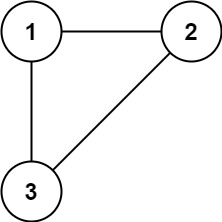
Input: edges = [[1,2],[1,3],[2,3]] Output: [2,3]
Example 2:
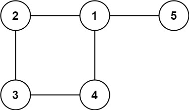
Input: edges = [[1,2],[2,3],[3,4],[1,4],[1,5]] Output: [1,4]
Constraints:
n =edges.length=3 <n <= 1000=edges[i].length =2=1 <a=i= < b=i= <= edges.length=a=_{=i}= != b=i- There are no repeated edges.
- The given graph is connected.
※ 2.12.13.1. Constraints and Edge Cases
- careful that the nodes are 1-indexed!
※ 2.12.13.2. My Solution (Code)
※ 2.12.13.2.1. [non-optimal, correct] v1: guided incremental BFS solution
This incrementally adds edges (as long as the nodes have been encountered before) and before adding each edge, checks if the nodes can already be reached. If they can already be reached, then this edge is redundant.
However, this is NOT the optimal solution, we have to do multiple DFS checks (via the helper can_reach for this).
1: from collections import defaultdict 2: 3: class Solution: 4: │ def findRedundantConnection(self, edges: List[List[int]]) -> List[int]: 5: │ │ adj = defaultdict(list) 6: │ │ 7: │ │ # check if we can reach dest from source 8: │ │ def can_reach(source, dest, visited): 9: │ │ │ # self loop: 10: │ │ │ if source == dest: 11: │ │ │ │ return True 12: │ │ │ │ 13: │ │ │ visited.add(source) 14: │ │ │ for nei in adj[source]: 15: │ │ │ │ # new neighbour 16: │ │ │ │ if nei not in visited: 17: │ │ │ │ │ if can_reach(nei, dest, visited): 18: │ │ │ │ │ │ return True 19: │ │ │ │ │ │ 20: │ │ │ return False 21: │ │ │ 22: │ │ for source, dest in edges: 23: │ │ │ visited = set() 24: │ │ │ # source, dest have both been encountered and 25: │ │ │ is_redundant = source in adj and dest in adj and can_reach(source, dest, visited) 26: │ │ │ if is_redundant: 27: │ │ │ │ return [source, dest] 28: │ │ │ │ 29: │ │ │ adj[source].append(dest) 30: │ │ │ adj[dest].append(source)
- Complexity Analysis:
- Time:
- For each edge, you might call
can_reach(DFS). - DFS may touch up to \(O(n)\) nodes (n=number of nodes < 1000).
- Since this can happen for up to \(O(n)\) edges, the total time is \(O(n^{2})\) in the worst case.
- For each edge, you might call
- Space:
- The adjacency list holds \(O(n)\) edges and \(O(n)\) nodes.
- The recursion stack in DFS is \(O(n)\) in the worst case.
- Time:
- Improvements:
can_reachcould have been namedis_connected- we don’t really need the
source in adj and dest in adjbecause the DFS will return false from node if it’s missing from the adj list
※ 2.12.13.2.2. [optimal] v2: Union Find
Intuition:
- Each node belongs to a “group” (set). Initially, every node is its own set.
- For each edge:
- If the nodes are already in the same set, this edge connects nodes already connected: this is the redundant edge! Return it.
- Otherwise, union the sets containing the two nodes (merge their components).
- This approach operates in nearly constant time per edge (amortized inverse Ackermann function via path compression and union by rank), so O(n) time.
1: class Solution: 2: │ def findRedundantConnection(self, edges: List[List[int]]) -> List[int]: 3: │ │ # parent lookup, starts with each being their own parent 4: │ │ parent = list(range(len(edges) + 1)) # since the nodes are 1-indexed 5: │ │ 6: │ │ def find(u): 7: │ │ │ # compress parent 8: │ │ │ while parent[u] != u: 9: │ │ │ │ # path compress to its own parent 10: │ │ │ │ parent[u] = parent[parent[u]] 11: │ │ │ │ u = parent[u] 12: │ │ │ │ 13: │ │ │ return u 14: │ │ │ 15: │ │ for u, v in edges: 16: │ │ │ # find parents of u and v: 17: │ │ │ pu, pv = find(u), find(v) 18: │ │ │ # if they're already connected, then this edge is redundant: 19: │ │ │ if pu == pv: 20: │ │ │ │ return [u, v] 21: │ │ │ │ 22: │ │ │ # mark them as having the same parent 23: │ │ │ parent[pu] = pv
I don’t like this variable naming, I prefer something that has a clearer structure of Union-Find and here’s a clearer version:
1: def findRedundantConnection(edges): 2: │ n = len(edges) 3: │ parent = [i for i in range(n+1)] 4: │ 5: │ def find(x): 6: │ │ while parent[x] != x: 7: │ │ │ # set grandparent as parent 8: │ │ │ parent[x] = parent[parent[x]] # path compression 9: │ │ │ # check grandparent 10: │ │ │ x = parent[x] 11: │ │ │ 12: │ │ return x 13: │ │ 14: │ def union(x, y): 15: │ │ rootX, rootY = find(x), find(y) 16: │ │ 17: │ │ if rootX == rootY: 18: │ │ │ return False # x and y are already connected 19: │ │ │ 20: │ │ parent[rootY] = rootX 21: │ │ return True 22: │ │ 23: │ for u, v in edges: 24: │ │ if not union(u, v): 25: │ │ │ return [u, v]
Some pointers:
Why does this give the last redundant edge?
You process edges in order; you always return on the first cycle detected, which aligns with the problem description, as the last edge detected (since all edges are unique, and you do not prematurely “fix” earlier cycles).
※ 2.12.13.3. My Approach/Explanation
My approach to this is to do BFS with edge-tracing
We have to build the adjacency list as we are processing the edges. For each edge, you want to see if its endpoints are already reachable using preceding edges only.
Before adding an edge \(u \leadsto v\), we do DFS to check if it can already be reached.
If so, then adding this edge makes it an extra edge, else just continue adding it in.
※ 2.12.13.4. My Learnings/Questions
- Intuition:
behind the DFS approach: For each new edge, you check (via DFS) before adding it: are the two endpoints already connected? If so, adding the edge would create a cycle—so it’s the redundant one.
If not, you add the edge to the adjacency list, keeping the graph up to date.
This ensures the last redundant edge is returned: because you process edges in order and return upon first detection of redundancy.
- Primer on Union Find
- Intuition
- You want to efficiently keep track of connectivity as the graph is built up.
- You want to answer: “Are these two nodes already connected BEFORE adding this edge?” fast!
- Union-Find does this quickly by representing everything with root ids—no need for full traversal.
- Intuition
- I couldn’t come up with the intuition for this, had to get guided. on hindsight the incremental addition is something I could have come up with if I had explored the incremental nature of this more. What threw me off was also the “If there are multiple answers” part, for which I had no mechanism I could think of that could apply to that.
※ 2.12.13.5. [Optional] Additional Context
This gave me a chance to deeper dive into union find algo.
※ 2.12.13.6. Retros
Ended up trying to write out the boilerplate, still need practice on the optimised union find.
Here, the even faster realisation is that we can just keep calling find, without needing to have a separate union function.
※ 2.12.14. [92] Word Ladder (127) hard almost wildcard_pattern_matching
A transformation sequence from word beginWord to word endWord
using a dictionary wordList is a sequence of words
beginWord -> s=_{=1}= -> s=2= -> … -> s=k such that:
- Every adjacent pair of words differs by a single letter.
- Every
s=_{=i} for1 <i <= k= is inwordList. Note thatbeginWorddoes not need to be inwordList. s=_{=k}== endWord
Given two words, beginWord and endWord, and a dictionary wordList,
return the number of words in the shortest transformation sequence
from beginWord to endWord=/, or/ =0 if no such sequence exists.
Example 1:
Input: beginWord = "hit", endWord = "cog", wordList = ["hot","dot","dog","lot","log","cog"] Output: 5 Explanation: One shortest transformation sequence is "hit" -> "hot" -> "dot" -> "dog" -> cog", which is 5 words long.
Example 2:
Input: beginWord = "hit", endWord = "cog", wordList = ["hot","dot","dog","lot","log"] Output: 0 Explanation: The endWord "cog" is not in wordList, therefore there is no valid transformation sequence.
Constraints:
1 <beginWord.length <= 10=endWord.length =beginWord.length=1 <wordList.length <= 5000=wordList[i].length =beginWord.length=beginWord,endWord, andwordList[i]consist of lowercase English letters.beginWord !endWord=- All the words in
wordListare unique.
※ 2.12.14.1. Constraints and Edge Cases
- remember that
beginWordmay not be in wordlist - type of edits: this question doesn’t consider additions or removals, just character replacements.
※ 2.12.14.2. My Solution (Code)
※ 2.12.14.2.1. [wrong] v1: close but wrong way to determine if should have an edge
1: from collections import defaultdict, deque 2: 3: class Solution: 4: │ def ladderLength(self, beginWord: str, endWord: str, wordList: List[str]) -> int: 5: │ │ wordSize = len(beginWord) 6: │ │ # maps word to adjacent words 7: │ │ adj = defaultdict(list) 8: │ │ 9: │ │ # make the edges: 10: │ │ # maps (i, j) => set diff 11: │ │ memo = defaultdict(int) 12: │ │ for i in range(len(wordList)): 13: │ │ │ for j in range(i + 1, len(wordList)): 14: │ │ │ │ shared_size = memo[(i, j)] 15: │ │ │ │ if not shared_size: 16: │ │ │ │ │ shared_size = len(set(wordList[i]) & set(wordList[j])) 17: │ │ │ │ │ memo[(i, j)] = shared_size 18: │ │ │ │ # if differs by one, then consider the edge: 19: │ │ │ │ if shared_size == wordSize - 1: 20: │ │ │ │ │ adj[wordList[i]].append(wordList[j]) 21: │ │ │ │ │ adj[wordList[j]].append(wordList[i]) 22: │ │ │ │ │ 23: │ │ # start searching from beginWord, it's a multi-source search 24: │ │ start_candidates = [(wordList[i], 0) for i in range(len(wordList)) if len(set(wordList[i]) & set(beginWord)) == 1] 25: │ │ 26: │ │ # now we do multi-source bfs: 27: │ │ queue = deque(start_candidates) 28: │ │ visited_words = set() 29: │ │ shortest_edits = float('inf') 30: │ │ while queue: 31: │ │ │ word, hop_count = queue.popleft() 32: │ │ │ if word == endWord: 33: │ │ │ │ shortest_edits = min(shortest_edits, hop_count) 34: │ │ │ │ continue 35: │ │ │ │ 36: │ │ │ for nei in adj[word]: 37: │ │ │ │ if nei in visited_words: 38: │ │ │ │ │ continue 39: │ │ │ │ │ 40: │ │ │ │ visited_words.add(nei) 41: │ │ │ │ queue.append((nei, hop_count + 1)) 42: │ │ │ │ 43: │ │ return 0 if shortest_edits > len(wordList) else shortest_edits
- Adjacency logic to determine if the edge should be added is NOT right
- You never include
beginWordin your adjacency graph (unless it’s already in wordList). You start search from words “adjacent” to beginWord, but for BFS it’s much cleaner to start from beginWord itself, at step 1.
Your queue starts from words “adjacent” to beginWord; this can cause it to miss shorter paths if transformations are possible in an order not found by your adjacency logic.
- BFS should return as soon as you find endWord; you don’t need to keep shortestedits/min, because BFS always finds the shortest path first.
Arithmetic issue:
You’re returning the hop count, but since output must include both beginWord and endWord, you should return
hop_count+1(because the starting word is also in the transformation sequence).
※ 2.12.14.2.2. [suboptimal, correct] v2: word-by-word adjacency approach \(O(n^{2})\)
1: from collections import deque, defaultdict 2: class Solution: 3: │ def ladderLength(self, beginWord: str, endWord: str, wordList: List[str]) -> int: 4: │ │ 5: │ │ wordSet = set(wordList) 6: │ │ if endWord not in wordSet: 7: │ │ │ return 0 8: │ │ │ 9: │ │ wordSet.add(beginWord) 10: │ │ adj = defaultdict(list) 11: │ │ 12: │ │ # only accept edge if one letter diff edit distance 13: │ │ def differsByOne(a, b): 14: │ │ │ diff = 0 15: │ │ │ for char_a, char_b in zip(a, b): 16: │ │ │ │ if char_a != char_b: 17: │ │ │ │ │ diff += 1 18: │ │ │ │ │ if diff > 1: 19: │ │ │ │ │ │ return False 20: │ │ │ │ │ │ 21: │ │ │ return diff == 1 22: │ │ │ 23: │ │ wordList2 = list(wordSet) 24: │ │ # all pairs edges, only those that are one-diff should be an edge: 25: │ │ for i in range(len(wordList2)): 26: │ │ │ for j in range(i + 1, len(wordList2)): 27: │ │ │ │ if differsByOne(wordList2[i], wordList2[j]): 28: │ │ │ │ │ adj[wordList2[i]].append(wordList2[j]) 29: │ │ │ │ │ adj[wordList2[j]].append(wordList2[i]) 30: │ │ │ │ │ 31: │ │ # we do BFS from start word: 32: │ │ # tuple: word, hop_count 33: │ │ queue = deque([(beginWord, 1)]) 34: │ │ visited = set([beginWord]) 35: │ │ while queue: 36: │ │ │ word, hop_count = queue.popleft() 37: │ │ │ if word == endWord: 38: │ │ │ │ return hop_count 39: │ │ │ for nei in adj[word]: 40: │ │ │ │ if nei in visited: 41: │ │ │ │ │ continue 42: │ │ │ │ visited.add(nei) 43: │ │ │ │ queue.append((nei, hop_count + 1)) 44: │ │ │ │ 45: │ │ return 0
※ 2.12.14.2.3. [optimal correct] v3: better adjacency graph construction
One of the slower parts of the previous v2 approach is the way we do the adjacency lookups.
The intuition behind its optimisation can be:
Classic: build all patterns by replacing each character with * and mapping those patterns to possible words.
Use generic intermediate forms (e.g., *ot for hot). With this, build a map from intermediate pattern to list of words.
For each word, possible neighbors are all words matching any of its generic patterns.
This reduces adjacency connection lookup from \(O(N^{2})\) to \(O(L N)\), where L is word length
1: from collections import defaultdict, deque 2: 3: class Solution: 4: │ def ladderLength(self, beginWord: str, endWord: str, wordList: List[str]) -> int: 5: │ │ if endWord not in wordList: 6: │ │ │ return 0 7: │ │ │ 8: │ │ L = len(beginWord) 9: │ │ 10: │ │ # better mapping: 11: │ │ pattern_to_words = defaultdict(list) 12: │ │ for word in wordList: 13: │ │ │ for i in range(L): 14: │ │ │ │ pattern = word[:i] + "*" + word[i + 1:] 15: │ │ │ │ pattern_to_words[pattern].append(word) 16: │ │ │ │ 17: │ │ # now we run BFS: 18: │ │ queue = deque([(beginWord, 1)]) 19: │ │ visited = set([beginWord]) 20: │ │ while queue: 21: │ │ │ word, level = queue.popleft() 22: │ │ │ for i in range(L): 23: │ │ │ │ pattern = word[:i] + "*" + word[i + 1:] 24: │ │ │ │ for nei in pattern_to_words[pattern]: 25: │ │ │ │ │ if nei == endWord: 26: │ │ │ │ │ │ return level + 1 27: │ │ │ │ │ if nei not in visited: 28: │ │ │ │ │ │ visited.add(nei) 29: │ │ │ │ │ │ queue.append((nei, level + 1)) 30: │ │ │ │ │ │ 31: │ │ │ │ # prevents repeat lookups 32: │ │ │ │ pattern_to_words[pattern] = [] 33: │ │ │ │ 34: │ │ return 0
- Key Notes:
- Each pattern (wildcard) is used only once per search path to avoid cycles.
- level (not hop) is incremented by 1 each time, counting all words in the sequence.
- As soon as endWord is found, return immediately.
※ 2.12.14.3. My Approach/Explanation
First I should create a graph where each node is a word and edges between nodes should only exist if there’s a single edit that can be done.
After constructing the graph, I see this as a multi-source BFS. The BFS should end (happy case) when we find the endWord and we need to keep track of the hops to update the minhops.
However, this is the inferior method, its runtime complexity is in \(O(N^{2})\)
※ 2.12.14.4. My Learnings/Questions
TRICK: the wildcard approach helps us to have a denser graph
pattern-mapping / wildcard approach is the standard, optimal solution for Word Ladder.
- For interview/production, remember that BFS always finds the shortest path in an unweighted graph—once you hit endWord, you’re done!
- Careful on these:
- Mistake in Calculating String edit distances:
if we use set intersection, we can get false positives because it doesn’t account for the relative position of the character.
Set intersection does not account for positions—just for letter occurrence!
this is a better way to judge that:
Show/Hide Python Code1: │ def differsByOne(a, b): 2: │ │ diff = 0 3: │ │ for x, y in zip(a, b): 4: │ │ │ if x != y: 5: │ │ │ │ diff += 1 6: │ │ │ if diff > 1: 7: │ │ │ │ return False 8: │ │ return diff == 1
- on the range of
j, it shouldn’t overlap with i - careful on what goes into the visited set (e.g. word vs tuple)
- remember to include the beginWord in the graph as well!WE need to be able to consider it as a legit word.
- Mistake in Calculating String edit distances:
※ 2.12.14.5. [Optional] Additional Context
Your understanding is close—you just needed to fix the adjacency/differ-by-one logic and embrace a slightly different BFS graph model.
※ 2.12.15. [D-1] Is Graph Bipartite (785) bipartite_graph
There is an undirected graph with n nodes, where each node is
numbered between 0 and n - 1. You are given a 2D array graph,
where graph[u] is an array of nodes that node u is adjacent to. More
formally, for each v in graph[u], there is an undirected edge
between node u and node v. The graph has the following properties:
- There are no self-edges (
graph[u]does not containu). - There are no parallel edges (
graph[u]does not contain duplicate values). - If
vis ingraph[u], thenuis ingraph[v](the graph is undirected). - The graph may not be connected, meaning there may be two nodes
uandvsuch that there is no path between them.
A graph is bipartite if the nodes can be partitioned into two
independent sets A and B such that every edge in the graph
connects a node in set A and a node in set B.
Return true if and only if it is bipartite.
Example 1:
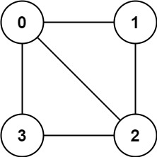
Input: graph = [[1,2,3],[0,2],[0,1,3],[0,2]] Output: false Explanation: There is no way to partition the nodes into two independent sets such that every edge connects a node in one and a node in the other.
Example 2:

Input: graph = [[1,3],[0,2],[1,3],[0,2]]
Output: true
Explanation: We can partition the nodes into two sets: {0, 2} and {1, 3}.
Constraints:
graph.length =n=1 <n <= 100=0 <graph[u].length < n=0 <graph[u][i] <= n - 1=graph[u]does not containu.- All the values of
graph[u]are unique. - If
graph[u]containsv, thengraph[v]containsu.
※ 2.12.15.1. Constraints and Edge Cases
- graph may be unconnected
- graph may have cycles. However, we don’t need to explicitly handle this.
※ 2.12.15.2. My Solution (Code)
1: class Solution: 2: │ def isBipartite(self, graph: List[List[int]]) -> bool: 3: │ │ # reminders: may be disconnected ==> just attempt to go through the unvisited ones 4: │ │ n = len(graph) 5: │ │ visited = [0] * n # value meaning: 0: unvisited, 1: colour A, 2: colour B 6: │ │ 7: │ │ # do an iterative DFS for each unvisited: 8: │ │ for idx in range(n): 9: │ │ │ if visited[idx] != 0: # visited already, carry on: 10: │ │ │ │ continue 11: │ │ │ stack = [idx] 12: │ │ │ visited[idx] = 1 # default colour? 13: │ │ │ 14: │ │ │ while stack: 15: │ │ │ │ node_idx = stack.pop() 16: │ │ │ │ node_colour = visited[node_idx] 17: │ │ │ │ 18: │ │ │ │ for nei in graph[node_idx]: 19: │ │ │ │ │ # case 1: same colour, violation: 20: │ │ │ │ │ if node_colour == visited[nei]: 21: │ │ │ │ │ │ return False 22: │ │ │ │ │ # case 3: uncoloured, start colouring 23: │ │ │ │ │ if visited[nei] == 0: 24: │ │ │ │ │ │ visited[nei] = 1 if node_colour == -1 else -1 25: │ │ │ │ │ │ stack.append(nei) 26: │ │ │ │ │ # case 2: different , carry on, do nothing 27: │ │ │ │ │ 28: │ │ return True
- Time Complexity:
- You visit each vertex once, and each edge once in an undirected graph → \(O(V + E)\).
- \(V\) = number of nodes (\(n\)), \(E\) = total edges.
- Space Complexity:
- visited array: \(O(V)\)
- Stack (DFS): up to \(O(V)\) in worst case (deep path).
- So total \(O(V)\) extra space.
Here’s a BFS version just for reference
1: from collections import deque 2: 3: class Solution: 4: │ def isBipartite(self, graph: List[List[int]]) -> bool: 5: │ │ n = len(graph) 6: │ │ color = [0] * n # 1: colour A, -1: colour B, 0: uncoloured 7: │ │ 8: │ │ for start in range(n): 9: │ │ │ if color[start] != 0: 10: │ │ │ │ continue 11: │ │ │ queue = deque([start]) 12: │ │ │ color[start] = 1 13: │ │ │ 14: │ │ │ while queue: 15: │ │ │ │ node = queue.popleft() 16: │ │ │ │ for nei in graph[node]: 17: │ │ │ │ │ if color[nei] == color[node]: 18: │ │ │ │ │ │ return False 19: │ │ │ │ │ if color[nei] == 0: 20: │ │ │ │ │ │ color[nei] = -color[node] 21: │ │ │ │ │ │ queue.append(nei) 22: │ │ return True
※ 2.12.15.3. My Approach/Explanation
2 graph colouring, uses DFS (pre order)
※ 2.12.15.4. My Learnings/Questions
- remember to:
- not forget to add to stack
- colour the root before continuing
※ 2.12.15.5. [Optional] Additional Context
This was a great confidence booster
※ 2.12.16. [D-2] Possible Bipartition (886) bipartite_graph
We want to split a group of n people (labeled from 1 to n) into
two groups of any size. Each person may dislike some other people, and
they should not go into the same group.
Given the integer n and the array dislikes where
dislikes[i] = [a=_{=i}=, b=i=]= indicates that the person labeled
a=_{=i} does not like the person labeled b=_{=i}, return true if
it is possible to split everyone into two groups in this way.
Example 1:
Input: n = 4, dislikes = [[1,2],[1,3],[2,4]] Output: true Explanation: The first group has [1,4], and the second group has [2,3].
Example 2:
Input: n = 3, dislikes = [[1,2],[1,3],[2,3]] Output: false Explanation: We need at least 3 groups to divide them. We cannot put them in two groups.
Constraints:
1 <n <= 2000=0 <dislikes.length <= 10=4dislikes[i].length =2=1 <a=i= < b=i= <= n=- All the pairs of
dislikesare unique.
※ 2.12.16.1. Constraints and Edge Cases
- remember that the graph is undirected
※ 2.12.16.2. My Solution (Code)
Just a bipartite check is alright,
1: from collections import defaultdict, deque 2: 3: class Solution: 4: │ def possibleBipartition(self, n: int, dislikes: List[List[int]]) -> bool: 5: │ │ # build adj list, disliker ==> disliked 6: │ │ adj = defaultdict(list) 7: │ │ for a, b in dislikes: 8: │ │ │ adj[a].append(b) 9: │ │ │ adj[b].append(a) 10: │ │ │ 11: │ │ # visited nodes, 0: unvisited, 1: colour A, -1: colour B 12: │ │ visited = [0] * (n + 1) 13: │ │ 14: │ │ for start_idx in range(1, n + 1): 15: │ │ │ if visited[start_idx]: 16: │ │ │ │ continue 17: │ │ │ │ 18: │ │ │ queue = deque([start_idx]) 19: │ │ │ 20: │ │ │ # colour start: 21: │ │ │ visited[start_idx] = 1 22: │ │ │ 23: │ │ │ while queue: 24: │ │ │ │ curr = queue.popleft() 25: │ │ │ │ curr_color = visited[curr] 26: │ │ │ │ 27: │ │ │ │ # colour neighbours: 28: │ │ │ │ for nei in adj[curr]: 29: │ │ │ │ │ if visited[nei] == curr_color: 30: │ │ │ │ │ │ return False 31: │ │ │ │ │ │ 32: │ │ │ │ │ if not visited[nei]: # uncoloured 33: │ │ │ │ │ │ visited[nei] = 1 if curr_color == -1 else -1 34: │ │ │ │ │ │ queue.append(nei) 35: │ │ │ │ │ │ 36: │ │ return True
※ 2.12.16.3. My Approach/Explanation
- this is just a bipartite check
- I just did a BFS here
※ 2.12.16.4. My Learnings/Questions
- technically we can simplify the flipping of the colour and just do
new = -old - use american english spelling just in case
Careful to check if it’s a directed or undirected graph. Here we have
adislikesb. It makes it seem as though it’s a directed graph.However, we are modelling incompatibility.
If
adislikesbthen BOTHaincompatible withbandbincompatible witha\(\implies\) we should treat it as an undirected graph and add in BOTH the edges.
※ 2.12.16.5. [Optional] Additional Context
I am SPEED.
It’s so fast to implement once I know the general approach that I need to take.
The specifics don’t have much friction here because I have a good mental model as well.
※ 2.13. 1-D DP
| Headline | Time | ||
|---|---|---|---|
| Total time | 7:49 | ||
| 1-D DP | 7:49 | ||
| [93] Climbing Stairs (70) | 0:05 | ||
| [94] Min Cost Climbing Stairs (746) | 0:18 | ||
| [95] House Robber I (198) | 0:18 | ||
| [96] House Robber II (213) | 0:27 | ||
| [97] ⭐️ Longest Palindromic Substring… | 1:35 | ||
| [98] Palindromic Substrings (647) | 0:10 | ||
| [99] Decode Ways (91) | 1:56 | ||
| [100] Coin Change (322) | 0:30 | ||
| [101] Maximum Product Subarray (152) | 1:16 | ||
| [102] Word Break (139) | 0:35 | ||
| [103] Longest Increasing Subsequence… | 0:39 |
※ 2.13.1. General Notes
※ 2.13.1.1. Fundamentals
For most of it, the notes written below (in the notes section) offer a deeper dive into things.
※ 2.13.1.1.1. Key Elements
- state transition equations
- will help us have an intuition on :
- what state to track? (this should be a common attribute that scaled down as we go into the subproblems e.g. count change -> the target amount left)
- what are the state dependencies like? This shows us how we should be tracking state changes from the \(i^{th}\) case and the \((i-1)^{th}\) case
- will help us have an intuition on :
optimal substructure
whether the optimal solution to the problem can be constructed from the optimal solutions to its subproblems
- thinking about this will help us gain intuition on :
- (carry on from above) what are the state dependencies like?
- what’s the minimum history we need to keep track of?
This affects the state-management apparati:
- bottom up approach: this influences the dimensions of our dp-array / table
- top-down approach: the parameters of the recursive function are used (we state-thread it).
- what choices are we making that will affect the state? what’s the option-pool like?
- after identifying the mechanism for the state keeping, we should be able to tell what a filled value in the table means. e.g. “dp[i] refers to the value of _ for the …”
- thinking about this will help us gain intuition on :
overlapping subproblems
to memoize and prevent unnecessary re-calculations
Thinking along these element gives the generic structure that we can expect
1: # Top-down recursive dynamic programming 2: def dp(state1, state2, ...): 3: │ for choice in all possible choices: 4: │ │ # The state changes after making the choice 5: │ │ result = find_optimal(result, dp(state1, state2, ...)) 6: │ return result 7: │ 8: # Bottom-up iterative dynamic programming 9: # Initialize base case 10: dp[0][0][...] = base case 11: # Perform state transitions 12: for state1 in all possible values of state1: 13: │ for state2 in all possible values of state2: 14: │ │ for ... 15: │ │ │ dp[state1][state2][...] = find_optimal(choice1, choice2, ...)
here’s an example, recursive solution with memoisation for the coin change problem
1: class Solution: 2: │ def __init__(self): 3: │ │ self.memo = [] 4: │ │ 5: │ def coinChange(self, coins: List[int], amount: int) -> int: 6: │ │ self.memo = [-666] * (amount + 1) 7: │ │ # Initialize the memo with a special value that won't be 8: │ │ # picked, representing it has not been calculated 9: │ │ return self.dp(coins, amount) 10: │ │ 11: │ def dp(self, coins, amount): 12: │ │ if amount == 0: return 0 13: │ │ if amount < 0: return -1 14: │ │ # Check the memo to prevent repeated calculations 15: │ │ if self.memo[amount] != -666: 16: │ │ │ return self.memo[amount] 17: │ │ │ 18: │ │ res = float('inf') 19: │ │ for coin in coins: 20: │ │ │ # Calculate the result of the subproblem 21: │ │ │ subProblem = self.dp(coins, amount - coin) 22: │ │ │ # Skip if the subproblem has no solution 23: │ │ │ if subProblem == -1: continue 24: │ │ │ # Choose the optimal solution from the subproblems and add one 25: │ │ │ res = min(res, subProblem + 1) 26: │ │ # Store the calculation result in the memo 27: │ │ self.memo[amount] = res if res != float('inf') else -1 28: │ │ return self.memo[amount]
and here’s the bottom up iterative version of it:
1: class Solution: 2: │ def coinChange(self, coins: List[int], amount: int) -> int: 3: │ │ # The array size is amount + 1, and the initial value is also amount + 1 4: │ │ dp = [amount + 1] * (amount + 1) 5: │ │ 6: │ │ dp[0] = 0 7: │ │ # base case 8: │ │ # The outer for loop is traversing all possible values of all states 9: │ │ for i in range(len(dp)): 10: │ │ │ # The inner for loop is finding the minimum value among all choices 11: │ │ │ for coin in coins: 12: │ │ │ │ # The subproblem has no solution, skip 13: │ │ │ │ if i - coin < 0: 14: │ │ │ │ │ continue 15: │ │ │ │ dp[i] = min(dp[i], 1 + dp[i - coin]) 16: │ │ │ │ 17: │ │ return -1 if dp[amount] == amount + 1 else dp[amount]
※ 2.13.1.1.2. Designing State Transitions and Relying on Mathematical Induction
The article suggests that it’s better to see the dp design as aspects of a proof by induction:
Assume the previous answers are known, use mathematical induction to correctly deduce and transition states, and ultimately arrive at the solution.
We assume we have the information and see how an optimal solution to the subproblem can be used to find the answer to the larger problem (similar to \(k^{th}\) case and \((k+1)^{th}\) case induction step).
For that to happen, the main dp array should be instrumental in giving us our answer. If it isn’t there’s a need to identify and build more auxiliary dp arrays for this.
※ 2.13.1.2. Tricks
※ 2.13.1.2.1. pythonic
- use
@lru_cacheor@cachefromfunctoolslibrary when doing function memoisations.
※ 2.13.1.2.2. Recurrence Formulas
- in the case of house robber II vs house robber I, we realise that it’s a matter of reducing the problem from circular to straight arrays. Literally just array splicing in the context of the contraints given.
In the case of Longest Palindromic Substring, it’s a matter of tracking contiguous regions which makes it feel 2-dimensional.
What are the 2 dimensions? Can we find equivalent but different ways of representing the state equations? Yes We can let the substrings (continugous) be defined by
left,rightpointers. We can ALSO let it be defined byleft, lengthinstead.
※ 2.13.1.3. Useful Algos
※ 2.13.1.3.1. Longest Palindromic Substring Search
- Intuition
- Every palindrome can be defined by its “center.”
- For each character (and the space between characters), treat it as a center and expand outwards as long as the substring is a palindrome.
- Handles both odd and even-length palindromes by considering:
- A single character as center (odd length)
- A pair between characters as center (even length).
- Process
- For each index `i` in string `s`, try to expand around:
- Center at `i` (for odd-length palindromes)
- Center between `i` and `i+1` (for even-length palindromes)
- While the substring `s[left:right+1]` remains a palindrome `s[left] == s[right]`, expand outwards.
- Track start and length of the longest palindromic substring found[1][2][4][5][6].
- For each index `i` in string `s`, try to expand around:
- Time/Space Complexity
- Time: O(n²) (expands for each possible center)
- Space: O(1)
Pythonic Example
Show/Hide Python Code│ def longestPalindrome(s): │ │ n = len(s) │ │ start, max_len = 0, 1 │ │ │ │ def expand_around_center(left, right): │ │ │ while left >= 0 and right < n and s[left] == s[right]: │ │ │ │ left -= 1 │ │ │ │ right += 1 │ │ │ return left + 1, right - 1 │ │ │ │ │ for i in range(n): │ │ │ l1, r1 = expand_around_center(i, i) │ │ │ l2, r2 = expand_around_center(i, i + 1) │ │ │ if r1 - l1 + 1 > max_len: │ │ │ │ start, max_len = l1, r1 - l1 + 1 │ │ │ if r2 - l2 + 1 > max_len: │ │ │ │ start, max_len = l2, r2 - l2 + 1 │ │ return s[start:start+max_len]
- Why it Works
- For string of length n, there are (2n-1) centers (n odd, n-1 even).
- Expanding around each yields all possible palindromic substrings.
- Intuition
- Fastest known algorithm: finds the longest palindromic substring in O(n) time and space[7][10].
- Uses the idea of palindromic symmetry and pre-processing.
- Treats all palindromes as odd length by inserting ’#’ or special chars between every real char and at boundaries.
- Process (Summary)
- Preprocess string: insert special chars (e.g., ’#’ between, ’^’ at start, ’\(' at end) to handle both odd/even-length centers uniformly (`"aba"` → `"^#a#b#a#\)"`).
- For each position in the new string, use previously calculated palindrome lengths to attempt to expand the palindrome centered at that position.
- Maintain a center `C` and a right boundary `R` of the current rightmost palindrome.
- For every new center, mirror its value using the palindrome around `C` if possible, and then try to expand further.
- Track the longest palindrome as you go[7][10].
- Time/Space Complexity
- Time: O(n)
- Space: O(n)
- Benefits/Drawbacks
- Extremely fast for very large inputs
- More complex to implement (hard for coding interviews unless specifically requested)
- Usually not needed for n ≤ 1000, but valuable to be aware of for advanced optimization[1].
Pseudocode
Show/Hide Python Code│ def manacher(s): │ │ T = '^#' + '#'.join(s) + '#$' │ │ n = len(T) │ │ P = [0] * n │ │ C = R = 0 │ │ for i in range(1, n-1): │ │ │ mirr = 2*C - i │ │ │ if i < R: │ │ │ │ P[i] = min(R - i, P[mirr]) │ │ │ # Expand palindrome centered at i │ │ │ while T[i + 1 + P[i]] == T[i - 1 - P[i]]: │ │ │ │ P[i] += 1 │ │ │ # Update center and right edge │ │ │ if i + P[i] > R: │ │ │ │ C, R = i, i + P[i] │ │ # Extract longest palindrome │ │ max_len = max(P) │ │ center = P.index(max_len) │ │ start = (center - max_len) // 2 │ │ return s[start:start + max_len]
※ 2.13.1.3.2. Patience Sorting for Longest Increasing Subsequence (\(O(nlogn)\)) hardhack
When doing LIS problems, we can find a linear time solution by using Patience sorting.
The easiest way to reason this is to just think about keeping track of piles of numbers that are increasing subsequences and just tracking the tail of that number.
A tail is the smallest value in that pile of numbers.
So we usually have 2 options for a particular number:
- it gets added to an existing pile
- it may possibly become a new tail within an existing pile
- it starts a new pile
- if the new number doesn’t fit with any of the existing tails (existing min values for the existing piles) then it should start a pile of its own.
Finally, we know that we can join up at least one element from each pile to form the longest increasing subsequence.
the code looks like this:
1: import bisect 2: class Solution: 3: │ def lengthOfLIS(self, nums: List[int]) -> int: 4: │ │ tails = [] 5: │ │ for x in nums: 6: │ │ │ # left most place to keep x within tails 7: │ │ │ # this picks the currently accumulating pile / stacks 8: │ │ │ # so tails[k] is giong t obe the smallest possible value of increasing subsequence of length (k + 1) 9: │ │ │ idx = bisect.bisect_left(tails, x) 10: │ │ │ if should_create_new_stack:=(idx == len(tails)): # can create a new stack 11: │ │ │ │ tails.append(x) 12: │ │ │ else: # replace within an existing stack's min (represents top of the stack) 13: │ │ │ │ tails[idx] = x 14: │ │ │ │ 15: │ │ return len(tails)
※ 2.13.1.4. Sources of Error
- typically we keep accumulating answers so we have \(k + 1\) table entries for example
MULTIPLYING NEGATIVE NUMBERS
for product-related accumulators, remember that we would likely have to handle both positive and negative accumulators (high, low) because if we do negative operands, then the negative value (low) might flip and become a large positive!
this is seen in the “Maxiumum Product Subarray” question.
- Filling order matters :
- we have to be keen on how the small instances get built. e.g. If we’re keeping track of lengths, then we can iterate over word-sizes and go from small to big.
※ 2.13.1.4.1. Misconceptions
it’s not true that whenever we see “contiguous” regions, we have to track BOTH the start and end regions and end up with a 2D table. We need to investigate deeper into what the structure/optimal substructure of the problem looks like.
Two pointers or 2D DP is required when you must explicitly consider all substring intervals, like Longest Palindromic Substring.
But here, since products multiply cumulatively, and the problem is one-dimensional with multiplicative “chain” structure, you can solve incrementally.
This is a classic example of 1D DP with constant space, where the state is “max/min product ending here”.
- In this case:
Maximum product ending at position i depends only on products ending at i-1 (not earlier).
These two values are enough because you don’t care about where the subarray started, only that it ends at i, and next step you move forward.
Therefore, it’s sufficient for us to just keep track of these:
max_ending_here: highest product of any subarray ending at index i.min_ending_here: similarly, lowest product ending at i (important because negative numbers can flip sign).
As for the substructure, this is it: \[\text{max}(nums[i], nums[i] * \text{max\_ending\_here}, nums[i] * \text{min\_ending\_here})\]
Why is tracking only max/min ending at i enough?
Because any subarray ending at i either:
- starts fresh at i (i.e., consists of just nums[i]), or
- extends a max or min subarray ending at i-1.
So you only need information about i-1 to determine i.
You don’t need to keep track of all possible start indices and subarray products.
- In this case:
- when attempting to rollup into 2 vars, the meaning of
curr,prevmight NOT be the same as before.
※ 2.13.2. [93] Climbing Stairs (70)
You are climbing a staircase. It takes n steps to reach the top.
Each time you can either climb 1 or 2 steps. In how many distinct
ways can you climb to the top?
Example 1:
Input: n = 2 Output: 2 Explanation: There are two ways to climb to the top. 1. 1 step + 1 step 2. 2 steps
Example 2:
Input: n = 3 Output: 3 Explanation: There are three ways to climb to the top. 1. 1 step + 1 step + 1 step 2. 1 step + 2 steps 3. 2 steps + 1 step
Constraints:
1 <n <= 45=
※ 2.13.2.1. Constraints and Edge Cases
Nothing fancy.
※ 2.13.2.2. My Solution (Code)
※ 2.13.2.2.1. [correct] v1: bottom up 1D DP approach
1: class Solution: 2: │ def climbStairs(self, n: int) -> int: 3: │ │ if n <= 2: 4: │ │ │ return n 5: │ │ │ 6: │ │ # init, where dp[i] == number of distinct ways to reach i 7: │ │ dp = [0] * n 8: │ │ 9: │ │ # base cases: 10: │ │ dp[0], dp[1] = 1, 2 11: │ │ 12: │ │ for i in range(2, n): 13: │ │ │ dp[i] = dp[i - 1] + dp[i - 2] 14: │ │ │ 15: │ │ return dp[n - 1]
Time: \(O(n)\) Space: \(O(n)\)
※ 2.13.2.2.2. [correct, optimised] v1.5: bottom up 1D dp approach, constant space
Technically we just need a history stack of size 2, instead of all n
1: class Solution: 2: │ def climbStairs(self, n: int) -> int: 3: │ │ if n <= 2: 4: │ │ │ return n 5: │ │ │ 6: │ │ prev, curr = 1, 2 7: │ │ for _ in range(3, n+1): 8: │ │ │ prev, curr = curr, prev + curr 9: │ │ │ 10: │ │ return curr 11:
Time: \(O(n)\) Space: \(O(1)\)
※ 2.13.2.2.3. [correct] v2: topdown recursive DP with memoization
Without memoization, top-down recursion is exponential (\(O(2^{n})\)), which would TLE for large n
Technically, this was too slow:
1: class Solution: 2: │ 3: │ def climbStairs(self, n: int) -> int: 4: │ │ if n <= 2: 5: │ │ │ return n 6: │ │ │ 7: │ │ return self.climbStairs(n - 1) + self.climbStairs(n - 2)
However, caching the function prevents unnecessary computations and it’s fast enough for the inputs:
1: from functools import lru_cache 2: 3: class Solution: 4: │ @lru_cache(None) 5: │ def climbStairs(self, n: int) -> int: 6: │ │ if n <= 2: 7: │ │ │ return n 8: │ │ │ 9: │ │ return self.climbStairs(n - 1) + self.climbStairs(n - 2) 10:
Time: \(O(n)\) Space: \(O(n)\)
※ 2.13.2.3. My Approach/Explanation
This is the classic description of recursive thinking that I personally use.
I prefer a bottom-up approach here. If we use a 1D array, dp[i] is the number of distinct ways to reach index i.
The base cases are just idx = 0 and idx = 1.
※ 2.13.2.4. My Learnings/Questions
- when planning the structure of the dp state management, remember to consider if there can be any pruning done. In this case, we just need a 2-variable history rather than an entire n-sized list to keep values.
- honestly this is just fibonacci
- pythonic improvements:
- Use range(3, n+1) so the code corresponds directly to step numbers for maximum clarity.
- Prefer dp = * (n+1) and return dp[n] for base-1 indexing, if matching the problem statement exactly.
- For exposure, different approaches:
- Mathematical (Binet’s Formula/Fibonacci Formula):
- Since this is just the Fibonacci sequence shifted by one (
dp[n] = Fib(n+1)), you could (very rarely in interviews) use a closed-form \(O(1)\) formula using the golden ratio and powers. - But this is rarely required, as integer rounding or precision can introduce subtle bugs.
- Since this is just the Fibonacci sequence shifted by one (
- Combinatorial Approach:
- Total number of ways = sum over k=0 to n//2 of C(n-k, k) (“choose k positions to place a 2-step, rest will be 1-steps”).
- Again, this is more math than programming, and not favored for interview code.
- Dynamic Programming Table (what you did):
- Standard, readable, preferred.
- Mathematical (Binet’s Formula/Fibonacci Formula):
※ 2.13.2.4.1. @lru_cache Decorator: Quick Primer
- A decorator from Python’s `functools` module.
- Automatically caches function results (“memoization”).
- LRU = “Least Recently Used”—when full, evicts oldest entries.
from functools import lru_cache @lru_cache(maxsize=128) def fibonacci(n): │ if n < 2: │ │ return n │ return fibonacci(n-1) + fibonacci(n-2)
- Calls with the same arguments are cached and fast.
- `maxsize`: Maximum number of results to cache (`None` = unlimited).
- `typed`: If True, cache type-sensitive (treats f(3) and f(3.0) as different).
- Dynamic programming/memoization (recursive DP, Fibonacci, etc).
- Repeatedly called pure/expensive functions.
- API/database queries (read-only, repeated).
- Game state evaluators or combinatoric calculators.
We could have just used @cache instead and it would have been just as performant.
the lru part only is a useful thing if we bound the cache size, @cache is unbounded by default and @lru_cache is optionally bounded.
| Alternative | When to Use |
|---|---|
| Manual `dict` | Full control/custom/complex key patterns |
| `@cache` (Python 3.9+) | Unlimited cache, no eviction |
| `cachetools`/`joblib` | Need TTL, disk cache, FIFO/LFU/LRU, etc. |
| 3rd-party (e.g. Redis) | Shared/persistent/distributed cache |
| `cachedproperty` | Cache at the instance (object) level |
| No cache | Non-deterministic or “side effect” functions |
- Functions’ arguments must be hashable (no `list`/`dict` unless changed to tuple/frozenset).
- Use only for pure functions; not for side-effect or stateful logic.
- Perfect for algorithm/DP/recursion questions.
- `@lrucache` is easy, efficient memoization for pure Python functions.
- Use for recursive DP, repeated expensive calls, or anything with overlapping subproblems.
- Use alternatives for more advanced persistence, eviction, or mutability needs.
※ 2.13.3. [94] Min Cost Climbing Stairs (746) cost_reference rolling_2_var_method
You are given an integer array cost where cost[i] is the cost of
i=^{=th} step on a staircase. Once you pay the cost, you can either
climb one or two steps.
You can either start from the step with index 0, or the step with
index 1.
Return the minimum cost to reach the top of the floor.
Example 1:
Input: cost = [10,15,20] Output: 15 Explanation: You will start at index 1. - Pay 15 and climb two steps to reach the top. The total cost is 15.
Example 2:
Input: cost = [1,100,1,1,1,100,1,1,100,1] Output: 6 Explanation: You will start at index 0. - Pay 1 and climb two steps to reach index 2. - Pay 1 and climb two steps to reach index 4. - Pay 1 and climb two steps to reach index 6. - Pay 1 and climb one step to reach index 7. - Pay 1 and climb two steps to reach index 9. - Pay 1 and climb one step to reach the top. The total cost is 6.
Constraints:
2 <cost.length <= 1000=0 <cost[i] <= 999=
※ 2.13.3.1. Constraints and Edge Cases
- nothing fancy, just need to comprehend the question correctly as to “reach this step == paid the costs of jumping from previous steps” and NOT “cost of landing on this step”
※ 2.13.3.2. My Solution (Code)
※ 2.13.3.2.1. [correct, optimal] v1: rolling two-variable bottom-up DP solution
1: class Solution: 2: │ def minCostClimbingStairs(self, cost: List[int]) -> int: 3: │ │ if len(cost) == 0: 4: │ │ │ return 0 5: │ │ if len(cost) == 1: 6: │ │ │ return cost[0] 7: │ │ │ 8: │ │ prev, curr = cost[0], cost[1] 9: │ │ for i in range(2, len(cost)): 10: │ │ │ prev, curr = curr, min(prev, curr) + cost[i] 11: │ │ │ 12: │ │ return min(prev, curr)
Base cases:
- idx = 0 and idx= 1 just use the same cost as the cost indices
※ 2.13.3.2.2. [correct, optimal] v2: recursive with memoisation (DP)
1: from functools import cache 2: class Solution: 3: │ def minCostClimbingStairs(self, cost: List[int]) -> int: 4: │ │ @cache 5: │ │ def min_cost(i): 6: │ │ │ if i < 2: return cost[i] 7: │ │ │ return cost[i] + min(min_cost(i-1), min_cost(i-2)) 8: │ │ n = len(cost) 9: │ │ 10: │ │ return min(min_cost(n-1), min_cost(n-2))
※ 2.13.3.3. My Approach/Explanation
Almost the same as the previous question.
However, it’s important to understand the question’s mechanisms well.
You do not need to land on the last step; you need the minimum cost of getting past the last step, so from either the last or second last step.
※ 2.13.3.4. My Learnings/Questions
Intuition: Every DP state depends just on the two most recent — classic sign you can reduce array DP to \(O(1)\) space.
Interpretation: You grasped the critical insight: “finish” is just past the end; last step or second last can both act as the launch pad.
No need for alternative data structures: For problems of this type (linear recurrence, two-way transitions), space-optimized DP is always best.
careful on the question interpretation
You do not need to land on the last step; you need the minimum cost of getting past the last step, so from either the last or second last step.
careful
just need to comprehend the question correctly as to “reach this step == paid the costs of jumping from previous steps” and NOT “cost of landing on this step”
※ 2.13.4. [95] House Robber I (198)
You are a professional robber planning to rob houses along a street. Each house has a certain amount of money stashed, the only constraint stopping you from robbing each of them is that adjacent houses have security systems connected and it will automatically contact the police if two adjacent houses were broken into on the same night.
Given an integer array nums representing the amount of money of each
house, return the maximum amount of money you can rob tonight without
alerting the police.
Example 1:
Input: nums = [1,2,3,1] Output: 4 Explanation: Rob house 1 (money = 1) and then rob house 3 (money = 3). Total amount you can rob = 1 + 3 = 4.
Example 2:
Input: nums = [2,7,9,3,1] Output: 12 Explanation: Rob house 1 (money = 2), rob house 3 (money = 9) and rob house 5 (money = 1). Total amount you can rob = 2 + 9 + 1 = 12.
Constraints:
1 <nums.length <= 100=0 <nums[i] <= 400=
※ 2.13.4.1. Constraints and Edge Cases
- the early returns depends on the number of base cases. Here we can early return
when not nums and when len =1=.
※ 2.13.4.2. My Solution (Code)
※ 2.13.4.2.1. [correct] v1: Rolling 2-variable Bottom up DP
1: class Solution: 2: │ def rob(self, nums: List[int]) -> int: 3: │ │ if not nums: 4: │ │ │ return 0 5: │ │ │ 6: │ │ if len(nums) == 1: 7: │ │ │ return nums[0] 8: │ │ │ 9: │ │ │ 10: │ │ prev, curr = nums[0], max(nums[1], nums[0]) 11: │ │ for i in range(2, len(nums)): 12: │ │ │ this = nums[i] 13: │ │ │ prev, curr = curr, max( 14: │ │ │ │ nums[i] + prev, # choose this house to rob 15: │ │ │ │ curr # don't choose this house to rob 16: │ │ │ │ ) 17: │ │ │ │ 18: │ │ return curr
※ 2.13.4.2.2. [correct] v2: Recursion with Memoisation
This is to illustrate that DP bottom up methods and top down recursive methods are equivalent.
1: from functools import cache 2: class Solution: 3: │ def rob(self, nums: List[int]) -> int: 4: │ │ n = len(nums) 5: │ │ @cache 6: │ │ def dp(i): 7: │ │ │ if i >= n: return 0 8: │ │ │ return max(nums[i] + dp(i+2), dp(i+1)) 9: │ │ return dp(0)
※ 2.13.4.3. My Approach/Explanation
My first thought actually made it more like a backtracking, where we choose or don’t choose a node, like in combinations.
On continued thinking, it’s clearer that for the nth house, we have 2 choices: rob this house or don’t rob it.
So our DP array needs to do it such that dp[i] best rob amount so far = max(choose house, don't choose house)
※ 2.13.4.4. My Learnings/Questions
- re-emphasis that DP bottom up and topdown recursive are equivalent.
※ 2.13.4.5. [Optional] Additional Context
I actually did it systematically and the main intuition came from when I asked the question of “how to find optimal substructure” which led to “what choices do i have to make and what are the state-implications of that?”
※ 2.13.4.6. Retros
※ 2.13.4.6.1.
- The base cases caught me off-guard, I had some silly errors there.
basically,
- we have trivial base cases: these are the n = 0 (trivially return 0) and n either 1 or 2. In which case just return max(nums)
for the init cases,
prev, curr = nums[0], max(nums[0], nums[1])the thing to think about it, when I consider the \(i^{th}\) house, what are my choices. I can choose to not rob (in which case, my value so far would have been the prev value). That’s why the
max(nums[0], nums[1])instead of justnums[1]
※ 2.13.5. [96] House Robber II (213) circular_dependencies number_of_subproblems
You are a professional robber planning to rob houses along a street. Each house has a certain amount of money stashed. All houses at this place are arranged in a circle. That means the first house is the neighbor of the last one. Meanwhile, adjacent houses have a security system connected, and it will automatically contact the police if two adjacent houses were broken into on the same night.
Given an integer array nums representing the amount of money of each
house, return the maximum amount of money you can rob tonight without
alerting the police.
Example 1:
Input: nums = [2,3,2] Output: 3 Explanation: You cannot rob house 1 (money = 2) and then rob house 3 (money = 2), because they are adjacent houses.
Example 2:
Input: nums = [1,2,3,1] Output: 4 Explanation: Rob house 1 (money = 1) and then rob house 3 (money = 3). Total amount you can rob = 1 + 3 = 4.
Example 3:
Input: nums = [1,2,3] Output: 3
Constraints:
1 <nums.length <= 100=0 <nums[i] <= 1000=
※ 2.13.5.1. Constraints and Edge Cases
Nothing fancy.
※ 2.13.5.2. My Solution (Code)
※ 2.13.5.2.1. [incomplete] v0: abandoned, missing key insight
This is without thinking about the 2 mutually exclusive subproblems part.
1: class Solution: 2: │ def rob(self, nums: List[int]) -> int: 3: │ │ if not nums: 4: │ │ │ return 0 5: │ │ │ 6: │ │ if nums == 1: 7: │ │ │ return nums[0] 8: │ │ │ 9: │ │ if nums == 2: 10: │ │ │ return max(nums) 11: │ │ │ 12: │ │ prev, curr = nums[0], max(nums[1], nums[0]) 13: │ │ for i in range(2, len(nums)): 14: │ │ │ this = nums[i] 15: │ │ │ prev, curr = curr, max( 16: │ │ │ │ nums[i] + prev, # choose this house to rob 17: │ │ │ │ curr # don't choose this house to rob 18: │ │ │ │ )
※ 2.13.5.2.2. [optimal working] v1: mutually exclusive subproblems to break into
1: class Solution: 2: │ def rob(self, nums: List[int]) -> int: 3: │ │ if not nums: 4: │ │ │ return 0 5: │ │ if len(nums) == 1: 6: │ │ │ return nums[0] 7: │ │ │ 8: │ │ def rob_straight(houses): 9: │ │ │ if len(houses) == 0: 10: │ │ │ │ return 0 11: │ │ │ │ 12: │ │ │ if len(houses) == 1: 13: │ │ │ │ return houses[0] 14: │ │ │ │ 15: │ │ │ prev, curr = houses[0], max(houses[1], houses[0]) 16: │ │ │ for i in range(2, len(houses)): 17: │ │ │ │ this = houses[i] 18: │ │ │ │ prev, curr = curr, max( 19: │ │ │ │ │ houses[i] + prev, # chose this house to rob 20: │ │ │ │ │ curr 21: │ │ │ │ ) 22: │ │ │ │ 23: │ │ │ return curr 24: │ │ │ 25: │ │ │ 26: │ │ │ 27: │ │ # get 1D maxes for the staight-lined version: 28: │ │ return max( 29: │ │ │ rob_straight(nums[1:]), # case 1: we choose last house, forgo first house 30: │ │ │ rob_straight(nums[:len(nums) - 1]), # case 2: we choose first house, forgo last house 31: │ │ )
※ 2.13.5.3. My Approach/Explanation
※ 2.13.5.4. My Learnings/Questions
TRICK / Key Intuition:
The circular dependency can be “broken” by splitting into mutually exclusive open intervals not including both ends.
for the straight version, we can simplify
from this:
Show/Hide Python Code1: │ │ def rob_straight(houses): 2: │ │ │ if len(houses) == 0: 3: │ │ │ │ return 0 4: │ │ │ │ 5: │ │ │ if len(houses) == 1: 6: │ │ │ │ return houses[0] 7: │ │ │ │ 8: │ │ │ prev, curr = houses[0], max(houses[1], houses[0]) 9: │ │ │ for i in range(2, len(houses)): 10: │ │ │ │ this = houses[i] 11: │ │ │ │ prev, curr = curr, max( 12: │ │ │ │ │ houses[i] + prev, # chose this house to rob 13: │ │ │ │ │ curr 14: │ │ │ │ ) 15: │ │ │ │ 16: │ │ │ return curr
into this:
Show/Hide Python Code1: def rob_straight(houses): 2: │ prev, curr = 0, 0 3: │ for amount in houses: 4: │ │ prev, curr = curr, max(prev + amount, curr) 5: │ return curr
TRICK: reducing a circular problem into a linear one
this problem seems to just teach us the value of identifying sub-problems.
In this case, there’s a circular dependency going on.
This yields 2 mutually exclusive cases:
- we choose first house and not last house
- we choose last house and not first house
We need the max of these 2 approaches, the rest of it is the same 1D dp problem.
※ 2.13.5.5. [Optional] Additional Context
I think this intuition was manageable to get, just had to break it down into what the circular dependency means.
※ 2.13.5.6. Retros
※ 2.13.5.6.1.
I realise that the first reach (correctly) is about problem-reduction.
What’s the new constraint that has been added compared to the previous version? It’s the looping of the array.
How can we reduce the problem to straight arrays?? We either include the first house and exclude the second house or we exclude the first house and include the second house
And we can just dp this twice.
※ 2.13.6. [97] ⭐️ Longest Palindromic Substring (5) 2D_DP Manachers_Algo
Given a string s, return the longest palindromic substring in
s.
Example 1:
Input: s = "babad" Output: "bab" Explanation: "aba" is also a valid answer.
Example 2:
Input: s = "cbbd" Output: "bb"
Constraints:
1 <s.length <= 1000=sconsist of only digits and English letters.
※ 2.13.6.1. Constraints and Edge Cases
<list constraints, input limits, or tricky edge cases here>
※ 2.13.6.2. My Solution (Code)
※ 2.13.6.2.1. [wrong, close] v0: correct structure, minor bugs
This is very close!!
1: class Solution: 2: │ def longestPalindrome(self, s: str) -> str: 3: │ │ if not s or len(s) == 1: 4: │ │ │ return s 5: │ │ │ 6: │ │ L = len(s) 7: │ │ 8: │ │ # we init the 2D DP table 9: │ │ dp = [[False] * L for i in range(L)] 10: │ │ 11: │ │ # range = [i, j) inclusive, exclusive 12: │ │ # trivial fills: 13: │ │ for i in range(L - 1): 14: │ │ │ for j in range(i + 1, L): 15: │ │ │ │ # single length are trivially true 16: │ │ │ │ if j - i == 1: 17: │ │ │ │ │ dp[i][j] = True 18: │ │ │ │ │ 19: │ │ longest = s[0], 1 20: │ │ 21: │ │ for i in range(L - 1): 22: │ │ │ for j in range(i + 1, L): 23: │ │ │ │ is_edge_chars_same = s[i] == s[j - 1] 24: │ │ │ │ is_substring_palindrome = dp[i + 1][j - 1] 25: │ │ │ │ 26: │ │ │ │ if is_edge_chars_same and is_substring_palindrome: 27: │ │ │ │ │ dp[i][j] = True 28: │ │ │ │ │ if (j - i) > longest[1]: 29: │ │ │ │ │ │ longest = (s[i:j], j - i) 30: │ │ │ │ │ │ 31: │ │ return longest[0]
- Trivial Case inits:
- need to init for single sized (this is actually handled correctly here)
Range representation:
The meaning of
dp[i][j]. Typically people use[i, j]inclusive so it would represent substrings[i:j+1]Filling order issues:
We need to be able to fill in small substrings first before filling in the larger ones, so the windows defined need to go from small to big.
Currently it does the opposite, so we might be reading values before it’s actually ready to read from that cell.
※ 2.13.6.2.2. [correct, slow] v1: DP correctly, fill correctly (guided)
1: class Solution: 2: │ def longestPalindrome(self, s: str) -> str: 3: │ │ if not s or len(s) == 1: 4: │ │ │ return s 5: │ │ │ 6: │ │ L = len(s) 7: │ │ # we init the 2D DP table 8: │ │ dp = [[False] * L for _ in range(L)] 9: │ │ # accumulator! 10: │ │ start, max_length = 0, 1 11: │ │ 12: │ │ # trival fill the single char substrings: 13: │ │ for i in range(L): 14: │ │ │ dp[i][i] = True 15: │ │ │ 16: │ │ # trivial fill the 2-char substrings: 17: │ │ for i in range(L - 1): 18: │ │ │ if s[i] == s[i + 1]: 19: │ │ │ │ dp[i][i + 1] = True 20: │ │ │ │ start, max_length = i, 2 21: │ │ │ │ 22: │ │ # smartly do the substring build, go from small to big so use a window length that expands: 23: │ │ for length in range(3, L + 1): 24: │ │ │ for start_idx in range(0, L - length + 1): 25: │ │ │ │ end_idx = start_idx + length - 1 26: │ │ │ │ # is palindrome: 27: │ │ │ │ if s[start_idx] == s[end_idx] and dp[start_idx + 1][end_idx - 1]: 28: │ │ │ │ │ dp[start_idx][end_idx] = True 29: │ │ │ │ │ start, max_length = start_idx, length 30: │ │ │ │ │ 31: │ │ return s[start: start + max_length]
- improvements:
we can handle the handling for the 2 length handling by doing this to the main loop:
Show/Hide Python Code1: │ │ for length in range(2, n+1): 2: │ │ │ │ for i in range(n - length + 1): 3: │ │ │ │ │ │ j = i + length - 1 4: │ │ │ │ │ │ if s[i] == s[j] and (length == 2 or dp[i+1][j-1]): 5: │ │ │ │ │ │ dp[i][j] = True 6: │ │ │ │ │ │ if length > max_length: 7: │ │ │ │ │ │ │ │ start, max_length = i, length 8:
- Complexity Analysis
- Time: \(O(n^{2})\)
- Two nested loops: For substring length \(\ell = 3\) to \(n\), and start index \(i\).
- Space: \(O(n^{2})\)
- 2D DP table
dp[i][j]for all substrings.
- 2D DP table
- Time: \(O(n^{2})\)
- This can be beaten in terms of time using expand around center.
※ 2.13.6.2.3. [correct, asymptotically same but practically faster] v2: Expand Around center
The key idea here is that all palindromes have a “middle” and that we can keep expanding outwards from a middle to identify which are these palindromes.
When we iterate through the list, any of them could be valid middle candidates.
1: class Solution: 2: │ def longestPalindrome(self, s: str) -> str: 3: │ │ n = len(s) 4: │ │ start, max_length = 0, 1 5: │ │ 6: │ │ def expand(l, r): 7: │ │ │ while l >= 0 and r < n and s[l] == s[r]: 8: │ │ │ │ l -= 1 9: │ │ │ │ r += 1 10: │ │ │ return l + 1, r - 1 11: │ │ │ 12: │ │ for i in range(n): 13: │ │ │ l1, r1 = expand(i, i) # Odd length 14: │ │ │ l2, r2 = expand(i, i + 1) # Even length 15: │ │ │ if r1 - l1 + 1 > max_length: 16: │ │ │ │ start, max_length = l1, r1 - l1 + 1 17: │ │ │ if r2 - l2 + 1 > max_length: 18: │ │ │ │ start, max_length = l2, r2 - l2 + 1 19: │ │ │ │ 20: │ │ return s[start:start + max_length] 21:
※ 2.13.6.3. My Approach/Explanation
Since it’s substring, the contiguous property is important.
What to track?
Likely 2 pointers need to be tracked that form the boundaries of the subs tring. It will end up being a 2D table.
So, dp[i][j] is True if substring s[i: j + 1] is a palindrome.
It’s independent because we can technically independently find out what to fill in each cell.
So when we fill up the table, we can just use this state function for it:
\[ dp[i][j] = \begin{cases} True & \text{if } s[i] == s[j] \text{ and } (j - i < 2 \text{ or } dp[i+1][j-1]) \\ False & \text{otherwise} \end{cases} \]
※ 2.13.6.4. My Learnings/Questions
- just use inclusive ranges for the dp table. So,
dp[i][j]means that we’re referring to the ranges[i:j + 1]. This makes the reasoning a little easier. - Alternatives: Expand around center and manacher’s algo are two alternatives, refer to the algos notes in the sections above
※ 2.13.6.5. [Optional] Additional Context
I think this is alright the dp application was almost well done, I had the right intuition and was asking the right questions to build up to the correct structure. The offbyone errors are what threw me off but that’s alright.
※ 2.13.6.6. Retros
※ 2.13.6.6.1.
the key learning when formulating the slow solution is to just think about how to get the recurrence out. The first reach seems to be \(i^{th}\) index related. Then we realise that there’s going to be too many overlapping problems.
That’s why we need to have a good way of building the numbers and length is that good way.
We can let the substrings (continugous) be defined by
left,rightpointers. We can ALSO let it be defined byleft, lengthinstead.With these params, we can build from length = 1 onwards.
- 2 learnings:
- using “proxy” params to the OG meanings
- thinking about HOW to build the values in a meaningful manner.
- 2 learnings:
※ 2.13.7. [98] Palindromic Substrings (647) 2D_DP
Given a string s, return the number of palindromic substrings in
it.
A string is a palindrome when it reads the same backward as forward.
A substring is a contiguous sequence of characters within the string.
Example 1:
Input: s = "abc" Output: 3 Explanation: Three palindromic strings: "a", "b", "c".
Example 2:
Input: s = "aaa" Output: 6 Explanation: Six palindromic strings: "a", "a", "a", "aa", "aa", "aaa".
Constraints:
1 <s.length <= 1000=sconsists of lowercase English letters.
※ 2.13.7.1. Constraints and Edge Cases
<list constraints, input limits, or tricky edge cases here>
※ 2.13.7.2. My Solution (Code)
※ 2.13.7.2.1. v1: [correct, slow] iterative bottom up 2D-DP solution in \(O(n^{2})\) time and space
1: class Solution: 2: │ def countSubstrings(self, s: str) -> int: 3: │ │ if not s: 4: │ │ │ return 0 5: │ │ │ 6: │ │ if len(s) == 1: 7: │ │ │ return 1 8: │ │ │ 9: │ │ L = len(s) 10: │ │ dp = [[False] * L for _ in range(L)] 11: │ │ count = 0 12: │ │ 13: │ │ # trivial fills: 14: │ │ for i in range(L): 15: │ │ │ dp[i][i] = True 16: │ │ │ count += 1 17: │ │ │ 18: │ │ for length in range(2, L + 1): 19: │ │ │ for start_idx in range(0, L - length + 1): 20: │ │ │ │ end_idx = start_idx + length - 1 21: │ │ │ │ if s[start_idx] == s[end_idx] and ( # same boundary chars 22: │ │ │ │ │ length == 2 # 2-sized substring will trivially be counted 23: │ │ │ │ │ or dp[start_idx + 1][end_idx - 1] # inner substring is a palindrome 24: │ │ │ │ ): 25: │ │ │ │ │ dp[start_idx][end_idx] = True 26: │ │ │ │ │ count += 1 27: │ │ return count 28:
※ 2.13.7.2.2. v2: [correct, faster] expand out version \(O(n^{2})\) but typically faster
This is modified from the previous example of expand out. It does what it needs to do.
1: class Solution: 2: │ def countSubstrings(self, s: str) -> int: 3: │ │ if not s: 4: │ │ │ return 0 5: │ │ │ 6: │ │ if len(s) == 1: 7: │ │ │ return 1 8: │ │ │ 9: │ │ L = len(s) 10: │ │ 11: │ │ def expand(l, r): 12: │ │ │ count = 0 13: │ │ │ 14: │ │ │ while is_palindrome:=(l >= 0 and r < L and s[l] == s[r]): 15: │ │ │ │ count += 1 16: │ │ │ │ # expand out 17: │ │ │ │ l -= 1 18: │ │ │ │ r += 1 19: │ │ │ return count 20: │ │ │ 21: │ │ # center idx 22: │ │ count = 0 23: │ │ for center_idx in range(L): 24: │ │ │ count += expand(center_idx, center_idx) # this is the odd-lengthed version 25: │ │ │ count += expand(center_idx, center_idx + 1) # this is the even lengthed version 26: │ │ │ 27: │ │ return count
Pointers:
- remember that both the even and odd lengthed versions need to be counted for!
Some improvements:
- we could just keep a single count and make all the helper s nested within each other.
This is a cleaned up version of the expand out approach (though I think some of the variable names can be improved to make it more readable):
1: class Solution: 2: │ def countSubstrings(self, s: str) -> int: 3: │ │ count = 0 4: │ │ n = len(s) 5: │ │ 6: │ │ def expand(left, right): 7: │ │ │ c = 0 8: │ │ │ while left >= 0 and right < n and s[left] == s[right]: 9: │ │ │ │ c += 1 10: │ │ │ │ left -= 1 11: │ │ │ │ right += 1 12: │ │ │ return c 13: │ │ │ 14: │ │ for i in range(n): 15: │ │ │ count += expand(i, i) # odd length palindromes 16: │ │ │ count += expand(i, i + 1) # even length palindromes 17: │ │ │ 18: │ │ return count
※ 2.13.7.3. My Approach/Explanation
- this approach is similar to the previous question, just that this time we are accumulating a different value (we accumulate the total palindrome count)
※ 2.13.7.4. My Learnings/Questions
- the expand out approach is actually quite intuitive.
- An advanced Manacher’s algorithm can find longest palindromic substring in \(O(n)\) time but does not count all palindromic substrings efficiently.
※ 2.13.7.5. [Optional] Additional Context
I was able to implement both the DFS and the expand out versions! This is great.
※ 2.13.8. [99] Decode Ways (91) redo 1D_DP rolling_2_var_method
You have intercepted a secret message encoded as a string of numbers. The message is decoded via the following mapping:
"1" -> 'A'
"2" -> 'B'
...
"25" -> 'Y'
"26" -> 'Z'
However, while decoding the message, you realize that there are many
different ways you can decode the message because some codes are
contained in other codes ("2" and "5" vs "25").
For example, "11106" can be decoded into:
"AAJF"with the grouping(1, 1, 10, 6)"KJF"with the grouping(11, 10, 6)- The grouping
(1, 11, 06)is invalid because"06"is not a valid code (only"6"is valid).
Note: there may be strings that are impossible to decode.
Given a string s containing only digits, return the number of ways to
decode it. If the entire string cannot be decoded in any valid way,
return 0.
The test cases are generated so that the answer fits in a 32-bit integer.
Example 1:
Input: s = “12”
Output: 2
Explanation:
“12” could be decoded as “AB” (1 2) or “L” (12).
Example 2:
Input: s = “226”
Output: 3
Explanation:
“226” could be decoded as “BZ” (2 26), “VF” (22 6), or “BBF” (2 2 6).
Example 3:
Input: s = “06”
Output: 0
Explanation:
“06” cannot be mapped to “F” because of the leading zero (“6” is different from “06”). In this case, the string is not a valid encoding, so return 0.
Constraints:
1 <s.length <= 100=scontains only digits and may contain leading zero(s).
※ 2.13.8.1. Constraints and Edge Cases
<list constraints, input limits, or tricky edge cases here>
※ 2.13.8.2. My Solution (Code)
※ 2.13.8.2.1. [Failed] V0: flailing attempt but kept the wrong state
1: class Solution: 2: │ def numDecodings(self, s: str) -> int: 3: │ │ # trivial invalidator for start string 4: │ │ if int(s[0]) == 0: 5: │ │ │ return 0 6: │ │ │ 7: │ │ L = len(s) 8: │ │ # dp[i] (can_solo, can_duo) 9: │ │ dp = [[] for _ in range(L)] 10: │ │ 11: │ │ is_duo = lambda idx: 1 <= idx < L and 9 < int(s[idx - 1: idx + 1]) < 27 12: │ │ is_solo = lambda idx: 0 <= idx < L and 1 < int(s[idx]) < 10 13: │ │ 14: │ │ count = 0 15: │ │ dp[0] = [True, False] 16: │ │ count += 1 17: │ │ 18: │ │ 19: │ │ for idx in range(1, L): 20: │ │ │ dp[idx] = [is_solo(idx), is_duo(idx)] 21: │ │ │ # if this idx can be both a solo and a duo then we have one more way to read this idx. 22: │ │ │ if dp[idx][0] and dp[idx][1]: 23: │ │ │ │ count += 2 24: │ │ │ │ 25: │ │ │ if (dp[idx][0] and not dp[idx][1]) or (dp[idx][1] and not dp[idx][0]): 26: │ │ │ │ count += 1 27: │ │ │ │ 28: │ │ │ if not dp[idx][0] and not dp[idx][1]: 29: │ │ │ │ return 0 30: │ │ │ │ 31: │ │ return count
This approach is actually not possible for us to rectify. Check out the explanation here:
The short answer is: **No, your revised version still fundamentally misses the way dynamic programming works for this problem and cannot be rectified simply by minor tweaks.** ### Why this approach still won’t work / cannot just be fixed: #### 1. **dp structure is wrong:** - You define `dp[i] = [can_solo, can_duo]` as booleans indicating whether the substring at `i` can be decoded as a single digit or two-digit code. - But your goal is **the number of ways to decode the substring** up to `i`, which needs to **accumulate counts from previous states**, not just record feasibility at position `i`. - Storing booleans about current character validity **does not track how many ways you got there**. #### 2. **Counting logic (`count`) is incorrect:** - You increase `count` based on whether the current position is valid as solo or duo. - But decoding ways depend on **how many ways you could decode preceding substrings**, not just current feasibility. - For example: │ - `"11"` can be decoded as "AA" or "K" → 2 ways. │ - Your code would add `count` based on local booleans but miss how multiple previous combinations create new paths. │ #### 3. **Lack of recurrence:** - The solution fundamentally requires **dp[i] to depend on dp[i-1] and dp[i-2]** counts. - Your code does no such accumulation—`count` just increases naively. #### 4. **Incorrect indices and checks** - Your lambda conditions still have `1 = 1: - If s[i-1] != '0': │ dp[i] += dp[i-1] - If s[i-2:i] between "10" and "26": │ dp[i] += dp[i-2] ``` This recurrence exploits **previous count states, not just local booleans.** ### Why it can't be "patched" Your approach tries to track validity but never tracks how many ways you reached that `i`th position. Without cumulative counts, you cannot return the correct answer. ## Conclusion - Your current approach is fundamentally incompatible with this problem. - The **correct DP must track counts** of ways cumulatively over prefix substrings. - Rectifying your code into a correct solution means rewriting with the standard DP counting approach, not patching booleans or local conditions. If you want, I can help rewrite your code into the correct counting DP approach—with detailed explanation and mapping to your style. Would you like that?
- DP State definition and meaning:
- usually we just keep number of ways to decode till \(i\) for \(dp[i]\), instead of keeping track of the bools that I have done it.
- You use
dp[i] = [bool, bool]to indicate whethers[i]can be decoded solo and/or duo. - However, for counting number of ways,
dp[i]should represent the number of ways to decode up to position i, not booleans. - You are mixing feasibility of decoding this position with accumulated counts, which breaks the DP logic.
- Incorrect count calculation
- Incrementing count by 1 or 2 per position based purely on booleans does not accumulate ways properly.
- For example, if a string is “111”, the number of ways is 3:
- “AAA” (1-1-1)
- “KA” (11-1)
- “AK” (1-11)
- Your code would not capture this dynamic accumulation.
- count should accumulate number of decoding ways based on previous dp states, not just current booleans.
- wrong dp size. Should just init to L + 1 to handle the empty case easily
※ 2.13.8.2.2. [correct, optimal] v1: corrected DP state tracking
1: class Solution: 2: │ def numDecodings(self, s: str) -> int: 3: │ │ # If the input is empty or starts with '0', there are no valid decodings. 4: │ │ if not s or s[0] == '0': 5: │ │ │ return 0 6: │ │ │ 7: │ │ L = len(s) 8: │ │ 9: │ │ # dp[i] will store the number of ways to decode the substring s[:i] 10: │ │ # We use length L + 1 to handle the base case for an empty substring 11: │ │ dp = [0] * (L + 1) 12: │ │ 13: │ │ # Base cases: 14: │ │ dp[0] = 1 # There's one way to decode an empty string (do nothing) 15: │ │ dp[1] = 1 # Since s[0] != '0', there's one way to decode the first character 16: │ │ 17: │ │ # Loop through the string from position 2 onwards (1-based indexing in dp) 18: │ │ for i in range(2, L + 1): 19: │ │ │ # Check if single digit decode is possible (last one digit) 20: │ │ │ # If s[i-1] is not '0', then we can decode it as a letter on its own 21: │ │ │ if s[i - 1] != '0': 22: │ │ │ │ dp[i] += dp[i - 1] # Add the ways up to the previous position 23: │ │ │ │ 24: │ │ │ # Check if two-digit decode is possible (last two digits) 25: │ │ │ two_digit = int(s[i - 2:i]) 26: │ │ │ # If the two-digit number is between 10 and 26 inclusive, it can be decoded as a letter 27: │ │ │ if 10 <= two_digit <= 26: 28: │ │ │ │ dp[i] += dp[i - 2] # Add the ways up to i - 2 position 29: │ │ │ │ 30: │ │ # The answer is the number of ways to decode the entire string s[:L] 31: │ │ return dp[L]
- Summary of implementation:
- Define
dp[i]as number of decoding ways up to indexi. - Proper base cases
dp[0] = 1(empty string) anddp[1] = 1(single-char string) depend on first char. - Build up dp with checks on one and two digit valid slices.
- Return
dp[n].
- Define
- Using the DP framework:
- Subproblems: Number of ways to decode substring `s[:i]`.
- Overlapping subproblems: Yes, decoding `s[:i]` depends on `s[:i-1]` and `s[:i-2]`.
- Choices at each subproblem: Decode single digit or two digits.
- DP Relation: \[ dp[i] = \mathbb{1}[s_{i-1} \neq 0] \cdot dp[i-1] + \mathbb{1}[10 \leq s_{i-2} s_{i-1} \leq 26] \cdot dp[i-2] \]
- Independence: Each choice leads to subproblems that do not interfere.
※ 2.13.8.2.3. [correct, optimised] v1.5: with two rolling variables
1: class Solution: 2: │ def numDecodings(self, s: str) -> int: 3: │ │ # Edge case: empty string or starting with '0' means no possible decoding 4: │ │ if not s or s[0] == '0': 5: │ │ │ return 0 6: │ │ │ 7: │ │ prev = 1 # dp[0], ways to decode empty string 8: │ │ curr = 1 # dp[1], ways to decode string of length 1 (assuming s[0] != '0') 9: │ │ 10: │ │ for i in range(1, len(s)): 11: │ │ │ temp = 0 # ways to decode up to position i+1 (1-based indexing) 12: │ │ │ 13: │ │ │ # Check if single digit decode is valid (s[i] != '0') 14: │ │ │ if s[i] != '0': 15: │ │ │ │ temp += curr # Can decode single char, so add ways till previous char 16: │ │ │ │ 17: │ │ │ # Check if two-digit decode is valid (10 <= s[i-1:i+1] <= 26) 18: │ │ │ two_digit = int(s[i-1:i+1]) 19: │ │ │ if 10 <= two_digit <= 26: 20: │ │ │ │ temp += prev # Can decode two chars together 21: │ │ │ │ 22: │ │ │ # If no valid decode for this position, temp will be 0 -> return 0 later 23: │ │ │ if temp == 0: 24: │ │ │ │ return 0 25: │ │ │ │ 26: │ │ │ # Shift dp states for next iteration 27: │ │ │ prev, curr = curr, temp 28: │ │ │ 29: │ │ return curr
- How it works:
prevstoresdp[i-2]— ways to decode string up to two characters before current index.currstoresdp[i-1]— ways to decode string up to one character before current index.- On each iteration, we compute the ways for substring ending at current index by looking at these two states.
- Rolling variables reduce space from \(O(n)\) to \(O(1)\).
※ 2.13.8.2.4. [correct, optimal] v2: top down recursive with caching / memo
1: from functools import cache 2: 3: class Solution: 4: │ def numDecodings(self, s: str) -> int: 5: │ │ n = len(s) 6: │ │ 7: │ │ @cache 8: │ │ def dfs(i): 9: │ │ │ if i == n: 10: │ │ │ │ return 1 # Finished decoding successfully 11: │ │ │ if s[i] == '0': 12: │ │ │ │ return 0 # Invalid 13: │ │ │ │ 14: │ │ │ # Single digit decode 15: │ │ │ count = dfs(i + 1) 16: │ │ │ 17: │ │ │ # Two digit decode if valid 18: │ │ │ if i + 1 < n and 10 <= int(s[i:i+2]) <= 26: 19: │ │ │ │ count += dfs(i + 2) 20: │ │ │ │ 21: │ │ │ return count 22: │ │ │ 23: │ │ return dfs(0)
※ 2.13.8.3. My Approach/Explanation
I think the rough idea for this is to just think simple.
The variable we need here is the count, which instead of being an accumulator, should be brought about by referring to our DP table.
※ 2.13.8.4. My Learnings/Questions
- comprehension: Not sure why but I interpreted it as “running approaches” and so didn’t think of it as a branching tree…
- tricks:
- init array with 1 extra to account for empty
You created
dp = [[] for _ in range(L)]but often DP arrays are sizedL+1to handle empty prefix easily.
- init array with 1 extra to account for empty
You created
※ 2.13.8.5. [Optional] Additional Context
I needed guidance for this, my initial intuition was wrong.
※ 2.13.8.6. Retros
※ 2.13.8.6.1.
- Got juked by this. Two things to note here:
dp[i]is best described as number of ways to decode the regions[:i], that’s why we dolen(dp) = n + 1at each
dp[i], we can either see it as a 1-fer or a 2-fer if 1-fer we adddp[i - 1]if 2-fer we adddp[i - 2]AND that’s how we can flatted into just
prevandcurrvar tracking.
So another learning is that the flatting / rolling into variables is not as trivial.
If we were to keep a n-lengthed DP array, then
dp[i]means the number of ways to decode the substrings[:i].However, now if we want to just keep
prevandcurr, thencurractualy refers to the index that JUST got calculated. So we should start our counting from s-idx 1 to n - 1 inclusive to get our answer.Here’s my re-attempted version with the variable roll-up.
Show/Hide Python Code1: class Solution: 2: │ def numDecodings(self, s: str) -> int: 3: │ │ # the main choice is whether i can be a one-fer or two-fer, if at all 4: │ │ # dp[i] = ith place how many 5: │ │ # recurrence: A) cannot 1fer and cannot 2-fer B) can 1 fer but not 2fer C: can 1fer or 2fer 6: │ │ 7: │ │ n = len(s) 8: │ │ if n == 1: 9: │ │ │ return 0 if s == '0' else 1 10: │ │ │ 11: │ │ # lmao random edge case, but can kind of make this up actually. 12: │ │ if n >= 2 and 1 <= int(s[:2]) <= 9: 13: │ │ │ return 0 14: │ │ │ 15: │ │ prev, curr = 1, 1 16: │ │ for i in range(1, n): # NOTE: here, i represents the calculation up to idx i of string s. so if we calculate i, means s[:i + 1] has been calculated. 17: │ │ │ can_2fer = 10 <= int(s[i - 1: i + 1]) <= 26 18: │ │ │ can_1fer = 1 <= int(s[i]) <= 9 19: │ │ │ 20: │ │ │ if not (can_2fer or can_1fer): 21: │ │ │ │ return 0 22: │ │ │ │ 23: │ │ │ prev, curr = curr, (prev if can_2fer else 0) + (curr if can_1fer else 0) 24: │ │ │ 25: │ │ return curr
※ 2.13.9. [100] Coin Change (322) DP recursive_top_down
You are given an integer array coins representing coins of different
denominations and an integer amount representing a total amount of
money.
Return the fewest number of coins that you need to make up that
amount. If that amount of money cannot be made up by any combination of
the coins, return -1.
You may assume that you have an infinite number of each kind of coin.
Example 1:
Input: coins = [1,2,5], amount = 11 Output: 3 Explanation: 11 = 5 + 5 + 1
Example 2:
Input: coins = [2], amount = 3 Output: -1
Example 3:
Input: coins = [1], amount = 0 Output: 0
Constraints:
1 <coins.length <= 12=1 <coins[i] <= 2=31= - 1=0 <amount <= 10=4
※ 2.13.9.1. Constraints and Edge Cases
Nothing fancy
※ 2.13.9.2. My Solution (Code)
※ 2.13.9.2.1. [correct, slow] Top down recursive DP
1: from functools import cache 2: class Solution: 3: │ def coinChange(self, coins: List[int], amount: int) -> int: 4: │ │ @cache 5: │ │ def helper(amount): 6: │ │ │ if amount == 0: 7: │ │ │ │ return 0 8: │ │ │ │ 9: │ │ │ if amount < 0: 10: │ │ │ │ return -1 11: │ │ │ │ 12: │ │ │ options = [helper(amount - denom) for denom in coins if 13: │ │ │ │ │ │ amount - denom >= 0 and helper(amount - denom) != -1] 14: │ │ │ │ │ │ 15: │ │ │ if not options: 16: │ │ │ │ return -1 17: │ │ │ else: 18: │ │ │ │ return min(options) + 1 19: │ │ │ │ 20: │ │ return helper(amount) 21:
- Explanation
- When
amount =0=, 0 coins needed. - When
amount < 0, return -1 (invalid). - For each coin, recursively get the min coins needed for
amount - coin. - Only consider results which are not -1.
- Return the minimum candidate or -1 if none found.
- When
※ 2.13.9.2.2. [correct, fast] iterative 1D DP
This works so much faster.
1: class Solution: 2: │ def coinChange(self, coins: List[int], amount: int) -> int: 3: │ │ # dp[i] will be the min number of coins to make amount == i 4: │ │ dp = [[-1] for _ in range(amount + 1)] # init value to be = sentinel 5: │ │ 6: │ │ dp[0] = 0 7: │ │ for denom in coins: 8: │ │ │ if denom > amount: 9: │ │ │ │ continue 10: │ │ │ dp[denom] = 1 11: │ │ │ 12: │ │ for amt in range(1, amount + 1): 13: │ │ │ options = [dp[amt - denom] for denom in coins if amt - denom >= 0 and dp[amt - denom] != -1] 14: │ │ │ if not options: 15: │ │ │ │ dp[amt] = -1 16: │ │ │ else: 17: │ │ │ │ dp[amt] = min(options) + 1 18: │ │ │ │ 19: │ │ return dp[amount]
Improvements:
- You do
dp = [[-1] for _ in range(amount+1)]which creates a list of lists, not just a list of ints — you probably wantdp = [-1] * (amount+1)instead.
Here’s a cleaned up version of my own implementation:
1: from functools import cache 2: class Solution: 3: │ def coinChange(self, coins: List[int], amount: int) -> int: 4: │ │ # dp[i] will be the min number of coins to make amount == i 5: │ │ dp = [-1] * (amount + 1) # init value to be = sentinel 6: │ │ 7: │ │ dp[0] = 0 8: │ │ for denom in coins: 9: │ │ │ if denom > amount: 10: │ │ │ │ continue 11: │ │ │ dp[denom] = 1 12: │ │ │ 13: │ │ for amt in range(1, amount + 1): 14: │ │ │ options = [dp[amt - denom] for denom in coins if amt - denom >= 0 and dp[amt - denom] != -1] 15: │ │ │ if not options: 16: │ │ │ │ dp[amt] = -1 17: │ │ │ else: 18: │ │ │ │ dp[amt] = min(options) + 1 19: │ │ │ │ 20: │ │ return dp[amount]
Here’s a cleaned up version of the optimal implementation:
1: class Solution: 2: │ def coinChange(self, coins: List[int], amount: int) -> int: 3: │ │ # This init of inf avoids negative values by using infinity, making code cleaner. 4: │ │ dp = [float('inf')] * (amount + 1) 5: │ │ dp[0] = 0 6: │ │ 7: │ │ for amt in range(1, amount + 1): 8: │ │ │ for coin in coins: 9: │ │ │ │ if coin <= amt: 10: │ │ │ │ │ dp[amt] = min(dp[amt], dp[amt - coin] + 1) 11: │ │ │ │ │ 12: │ │ return dp[amount] if dp[amount] != float('inf') else -1 13:
| Step | Explanation | Status/Notes |
|---|---|---|
| 1. Define Subproblems | Number of coins needed to form amount <= target amount | dp[i] = min coins needed for amount i |
| 2. Check Overlapping Subproblems | dp[i] depends on solutions of dp[i - coin] for each coin | Yes, overlapping subproblems exist |
| 3. Identify Choices Per Subproblem | Choose any coin from coins that fits into current amount | Multiple choices per state |
| 4. Confirm Optimal Substructure | Optimal for amount i computed from optimal solutions for smaller amounts | Yes, minimum over choices is optimal |
| 5. Compute Solution (Top-Down / Bottom-Up) | Bottom-up iterative or top-down memoized recursion both applicable | Both implemented correctly |
| 6. (Optional) Construct Actual Solution | Can store chosen coins to reconstruct path | Not implemented in provided solutions |
※ 2.13.9.3. My Approach/Explanation
For practice sake, I choose to do this via a recursive top down approach.
The DP state to track is the target amount, we use a helper and cache the helper.
I ended up implementing the bottom up iterative version as well.
※ 2.13.9.4. My Learnings/Questions
- the candidates / options part is very reminiscent of decision trees!
- for the DP array, I ended up following 1-index so that the answer will be at
dp[amount]. I think I’m getting the hang of how to structure the dp array for 1D dp.
※ 2.13.9.5. [Optional] Additional Context
I managed to do both version successfully! pretty happy.
※ 2.13.9.6. Retros
※ 2.13.9.6.1.
This was nice.
It’s DP because it’s arbitrary denominations and unlimited amounts of it. If a fixed amount, then it’s more of a greedy solution because we just pick the best possible that gives the biggest jump.
We also had to do the options checking to determine whether dp[i] could even be reached, the iterative solution is my favourite now, though the recursive one is faster to write out.
※ 2.13.10. [101] Maximum Product Subarray (152) redo rolling_2_var_method 1D_DP
Given an integer array nums, find a subarray that has the largest
product, and return the product.
The test cases are generated so that the answer will fit in a 32-bit integer.
Example 1:
Input: nums = [2,3,-2,4] Output: 6 Explanation: [2,3] has the largest product 6.
Example 2:
Input: nums = [-2,0,-1] Output: 0 Explanation: The result cannot be 2, because [-2,-1] is not a subarray.
Constraints:
1 <nums.length <= 2 * 10=4-10 <nums[i] <= 10=- The product of any subarray of
numsis guaranteed to fit in a 32-bit integer.
※ 2.13.10.1. Constraints and Edge Cases
- need to track negative accumulations because we can have two negatives that make a positive.
※ 2.13.10.2. My Solution (Code)
※ 2.13.10.2.1. [wrong, slow, missing edge cases] v1: 2D DP Table filling
1: class Solution: 2: │ def maxProduct(self, nums: List[int]) -> int: 3: │ │ n = len(nums) 4: │ │ # dp[i][j] would be the largest product within this window. Windows will overlap 5: │ │ # use inclusive ranges 6: │ │ # answer will be from accumulator prod 7: │ │ dp = [[1] * n for _ in range(n)] 8: │ │ 9: │ │ prod = -float('inf') 10: │ │ 11: │ │ # trivial fill the window size = 1 12: │ │ for i in range(n): 13: │ │ │ dp[i][i] = nums[i] 14: │ │ │ prod = max(prod, nums[i]) 15: │ │ │ 16: │ │ # main fills: 17: │ │ for length in range(2, n): 18: │ │ │ # i is the start of the window 19: │ │ │ for i in range((n - length) + 1): 20: │ │ │ │ # j is the end of the window 21: │ │ │ │ j = i + length - 1 22: │ │ │ │ val = dp[i][j - 1] * nums[j] 23: │ │ │ │ prod = max(prod, val) 24: │ │ │ │ dp[i][j] = val 25: │ │ │ │ 26: │ │ return prod
※ 2.13.10.2.2. [Correct, optimal] v2: 1D DP Table Filling with min and max tracking
You do not need explicit two pointers or a 2D DP table because the maximum product subarray ending at index i depends only on max/min products ending at i-1.
By tracking just those two variables at each step, you integrate the contribution of all contiguous subarrays ending there and keep the global max in O(n) time and O(1) space.
1: class Solution: 2: │ def maxProduct(self, nums: List[int]) -> int: 3: │ │ n = len(nums) 4: │ │ curr_max, curr_min = nums[0], nums[0] 5: │ │ result = curr_max 6: │ │ 7: │ │ for idx in range(1,len(nums)): 8: │ │ │ num = nums[idx] 9: │ │ │ # negative multiplication, will swap the min and max values 10: │ │ │ if num < 0: 11: │ │ │ │ curr_min, curr_max = curr_max, curr_min 12: │ │ │ │ 13: │ │ │ # max of (starting fresh, or accumulating) 14: │ │ │ curr_max = max(num, curr_max * num) 15: │ │ │ curr_min = min(num, curr_min * num) 16: │ │ │ 17: │ │ │ result = max(result, curr_max) 18: │ │ │ 19: │ │ return result
※ 2.13.10.3. My Approach/Explanation
The initial intuition is to immediately think of a 2 dimensional approach because subarrays would imply that I need to look at left, right pointers ( or left and length ).
The reason why we don’t need to do this is that they’re just asking us for an accumulated / encountered max.
We just need to keep in mind that negatives should be tracked as well.
※ 2.13.10.4. My Learnings/Questions
- 🚩 MAIN PITFALL:
Need to handle negative numbers well! I shall regard this as an input edge case that hasn’t been considered yet.
- Maximum product subarray is tricky because multiplication by negative numbers can turn smallest product into largest and vice versa.
- You need to track both maximum product and minimum product at each step (because a negative times a negative may become max).
- Your DP only stores the maximum product for each subarray, so it misses minimum (negative) products that can flip into a larger product further along.
- Misconception:
it’s not true that whenever we see “contiguous” regions, we have to track BOTH the start and end regions and end up with a 2D table. We need to investigate deeper into what the structure/optimal substructure of the problem looks like.
Two pointers or 2D DP is required when you must explicitly consider all substring intervals, like Longest Palindromic Substring.
But here, since products multiply cumulatively, and the problem is one-dimensional with multiplicative “chain” structure, you can solve incrementally.
This is a classic example of 1D DP with constant space, where the state is “max/min product ending here”.
- In this case:
Maximum product ending at position i depends only on products ending at i-1 (not earlier).
These two values are enough because you don’t care about where the subarray started, only that it ends at i, and next step you move forward.
Therefore, it’s sufficient for us to just keep track of these:
max_ending_here: highest product of any subarray ending at index i.min_ending_here: similarly, lowest product ending at i (important because negative numbers can flip sign).
As for the substructure, this is it: \[\text{max}(nums[i], nums[i] * \text{max\_ending\_here}, nums[i] * \text{min\_ending\_here})\]
Why is tracking only max/min ending at i enough?
Because any subarray ending at i either:
- starts fresh at i (i.e., consists of just nums[i]), or
- extends a max or min subarray ending at i-1.
So you only need information about i-1 to determine i.
You don’t need to keep track of all possible start indices and subarray products.
※ 2.13.10.5. [Optional] Additional Context
I didn’t methodically think it through, that’s why I only ended up getting the naive approach. That’s not ideal.
※ 2.13.10.6. Retros
※ 2.13.10.6.1.
The 1D approach makes sense because we just need to keep accumulator variables for max and min (for neg values).
I think it’s possible to come to this conclusion after initially entertaining a 2D approach because of the nature of contiguous regions (subarrays).
I think the main math property here is that multiplication is cumulative.
※ 2.13.11. [102] Word Break (139) 1D_DP 2_pointers
Given a string s and a dictionary of strings wordDict, return true
if s can be segmented into a space-separated sequence of one or more
dictionary words.
Note that the same word in the dictionary may be reused multiple times in the segmentation.
Example 1:
Input: s = "leetcode", wordDict = ["leet","code"] Output: true Explanation: Return true because "leetcode" can be segmented as "leet code".
Example 2:
Input: s = "applepenapple", wordDict = ["apple","pen"] Output: true Explanation: Return true because "applepenapple" can be segmented as "apple pen apple". Note that you are allowed to reuse a dictionary word.
Example 3:
Input: s = "catsandog", wordDict = ["cats","dog","sand","and","cat"] Output: false
Constraints:
1 <s.length <= 300=1 <wordDict.length <= 1000=1 <wordDict[i].length <= 20=sandwordDict[i]consist of only lowercase English letters.- All the strings of
wordDictare unique.
※ 2.13.11.1. Constraints and Edge Cases
- base case is trivially true where empty string is segmentable.
- nothing fancy
※ 2.13.11.2. My Solution (Code)
※ 2.13.11.2.1. v1: [correct] 1D DP
1: class Solution: 2: │ def wordBreak(self, s: str, wordDict: List[str]) -> bool: 3: │ │ L = len(s) 4: │ │ words = set(wordDict) # for fast membership checks 5: │ │ 6: │ │ # dp[i] is whether it's segmentable at ith idx 7: │ │ dp = [False] * (L + 1) # answer will be at dp[L] 8: │ │ # trivial base cases 9: │ │ # trivially true 10: │ │ dp[0] = True 11: │ │ 12: │ │ # leading pointer, right exclusive for the slicing 13: │ │ for right_idx in range(1, L + 1): 14: │ │ │ # for the left pointer 15: │ │ │ for left_idx in range(right_idx): 16: │ │ │ │ if not dp[left_idx]: 17: │ │ │ │ │ continue 18: │ │ │ │ │ 19: │ │ │ │ if s[left_idx:right_idx] in words: 20: │ │ │ │ │ dp[right_idx] = True 21: │ │ │ │ │ 22: │ │ return dp[L]
- Approach:
dp[i]meaning: whether the substrings[:i]can be segmented into dictionary words.- Base case:
dp[0] = Truefor the empty string. - For each
right_idx (1 to len(s)), you iterate over all possibleleft_idx < right_idx. - You check
if dp[left_idx] is True(the prefix up toleft_idxis valid) ands[left_idx:right_idx]is in the dictionary. - If both conditions are met, mark
dp[right_idx] = True.
- Improvements
※ 2.13.11.2.2. v2: [optimised v1] 1D DP
Just do early returns by using the max word length in the dictionary.
1: class Solution: 2: │ def wordBreak(self, s: str, wordDict: List[str]) -> bool: 3: │ │ wordSet = set(wordDict) # O(1) lookup 4: │ │ n = len(s) 5: │ │ dp = [False] * (n + 1) 6: │ │ dp[0] = True # empty substring is segmentable 7: │ │ 8: │ │ max_word_length = max(map(len, wordDict)) if wordDict else 0 9: │ │ 10: │ │ for i in range(1, n + 1): 11: │ │ │ # Limit left boundary to speed up checks (optimization) 12: │ │ │ for j in range(max(0, i - max_word_length), i): 13: │ │ │ │ if dp[j] and s[j:i] in wordSet: 14: │ │ │ │ │ dp[i] = True 15: │ │ │ │ │ break # early break for efficiency, since we know that dp[i] is already a legit segmentation. 16: │ │ │ │ │ 17: │ │ return dp[n]
※ 2.13.11.3. My Approach/Explanation
The substructure property is as such, if my last segment I can make from the right is legit, and the immediate left of that is also a valid segment then I’m fine with the whole segmentation process.
This would mean that my dp[i] keeps track of whether a valid segment ends at ith idx.
I can just keep building the bool array from the left. For each region I can find, I’m concerned with whether that substring boundaried by the region is within the wordlist. If I can find one such, then the right pointer is a valid segmentation pointer.
※ 2.13.11.4. My Learnings/Questions
- My weakness is really the boundaries to be set. Not sure why I’m not serious enough about getting the boundaries right.
- base case is trivially true where empty string is segmentable.
- Some pruning improvements:
Precompute max length of words to limit search:
Store
max_word_lento reduce inner loop range.Only check
left_idx in [right_idx - max_word_len, right_idx)instead of all. Fix the max window size!retro learning: we can do the same for min length as well
Show/Hide Python Code1: │ │ # we store dp[i] as bool for if we can segment s[:i] 2: │ │ for i in range(1, n + 1): # i is the right ptr 3: │ │ │ start = max(0, i - max_l) # check starting from max_l distance away 4: │ │ │ end = i - min_l + 1 # micro optimisation, check until min length distance away 5: │ │ │ for j in range(start, end): 6: │ │ │ │ if is_segmentable:=(dp[j] and s[j:i] in word_set): 7: │ │ │ │ │ dp[i] = True 8: │ │ │ │ │ break # carry on with next i iteration
QQ: For my V1, it’s NOT possible for me to return early from the substring loop right, because I should be trying to get info about segmentation from all possible words from wordlist, this will give flexibility.
AA: Yes, you can safely break once you find a valid partition for
dp[right_idx]. You still explore all ranges in outer loops, so no segments are skipped.
※ 2.13.11.5. [Optional] Additional Context
Much better here! Going to call it a nigght.
※ 2.13.11.6. Retro
※ 2.13.11.6.1.
Nicely done, I found a micro optimisation as well.
Instead of just limiting the left pointer to be max length ONLY, we can also limit the range of possible left pointer to consider min length in wordlist
1: class Solution: 2: │ def wordBreak(self, s: str, wordDict: List[str]) -> bool: 3: │ │ word_set = set(wordDict) # O(1) lookup 4: │ │ n = len(s) 5: │ │ dp = [False] * (n + 1) 6: │ │ dp[0] = True # empty substring is segmentable 7: │ │ 8: │ │ lengths = [len(word) for word in word_set] 9: │ │ min_l, max_l = min(lengths), max(lengths) 10: │ │ 11: │ │ # we store dp[i] as bool for if we can segment s[:i] 12: │ │ for i in range(1, n + 1): # i is the right ptr 13: │ │ │ for j in range(max(0, i - max_l), # check starting from max_l distance away 14: │ │ │ │ │ │ │ i - min_l + 1 # micro optimisation, check until min length distance away 15: │ │ │ │ │ │ │ ): 16: │ │ │ │ if is_segmentable:=(dp[j] and s[j:i] in word_set): 17: │ │ │ │ │ dp[i] = True 18: │ │ │ │ │ break # carry on with next i iteration 19: │ │ │ │ │ 20: │ │ return dp[n] 21:
- careful on the variable swapping
※ 2.13.12. [103] Longest Increasing Subsequence (300) 1D_DP patience_tracking_algo
Given an integer array nums, return the length of the longest
strictly increasing subsequence.
Example 1:
Input: nums = [10,9,2,5,3,7,101,18] Output: 4 Explanation: The longest increasing subsequence is [2,3,7,101], therefore the length is 4.
Example 2:
Input: nums = [0,1,0,3,2,3] Output: 4
Example 3:
Input: nums = [7,7,7,7,7,7,7] Output: 1
Constraints:
1 <nums.length <= 2500=-10=^{=4}= <= nums[i] <= 10=4
Follow up: Can you come up with an algorithm that runs
in O(n log(n)) time complexity?
※ 2.13.12.1. Constraints and Edge Cases
nothing fancy here
※ 2.13.12.2. My Solution (Code)
※ 2.13.12.2.1. v1 [correct, slow] 1D DP \(O(N^{2})\)
1: class Solution: 2: │ def lengthOfLIS(self, nums: List[int]) -> int: 3: │ │ n = len(nums) 4: │ │ # all init base to 1 5: │ │ dp = [1] * (n) 6: │ │ for right in range(1, n): 7: │ │ │ for left in range(right): 8: │ │ │ │ # we have this window and we need to find out if nums[right] can be incremented (if any smaller elements exist in the window) 9: │ │ │ │ if nums[right] > nums[left]: 10: │ │ │ │ │ dp[right] = max(dp[right], dp[left] + 1) 11: │ │ │ │ │ 12: │ │ return max(dp)
Your \(O(N^{2})\) solution using 1D DP is correct.
The array dp[i] stores the length of the longest increasing subsequence ending at nums[i].
For each nums[right], you consider all previous nums[left] where nums[right] > nums[left] and update dp[right] appropriately.
At the end, max(dp) correctly finds the length of the LIS.
※ 2.13.12.2.2. v2 [optimal, fast] Patience Sorting Algo \(O(N log N)\) time
1: import bisect 2: 3: class Solution: 4: │ def lengthOfLIS(self, nums: List[int]) -> int: 5: │ │ tails = [] # tails[i] will hold the smallest ending number of an increasing subsequence of length i+1 (tail of a stack of cards) 6: │ │ 7: │ │ for x in nums: 8: │ │ │ # Find the insertion point for x in tails to maintain sorted order 9: │ │ │ # This corresponds to the leftmost pile top >= x (or new pile if none found) 10: │ │ │ idx = bisect.bisect_left(tails, x) 11: │ │ │ 12: │ │ │ # CASE 1: add new pile: 13: │ │ │ # If x is larger than all pile tops, create a new pile by appending it 14: │ │ │ if idx == len(tails): 15: │ │ │ │ tails.append(x) 16: │ │ │ else: 17: │ │ │ │ # CASE 2: replace within existing stack: 18: │ │ │ │ # Otherwise, replace the existing pile top with x 19: │ │ │ │ # This keeps tails optimized to have smallest possible tail elements 20: │ │ │ │ tails[idx] = x 21: │ │ │ │ 22: │ │ # Number of piles equals length of longest increasing subsequence 23: │ │ return len(tails)
※ 2.13.12.3. My Approach/Explanation
I’ve seen this question before, so it’s a little biased.
For the substructure identification, we realise that we can just keep counts of the longest increasing subsequence within dp[i] and we can keep sweeping to increment values if we find any.
※ 2.13.12.4. My Learnings/Questions
- the patience algo version is so non intuitive! The only thing I can think of is that there’s a bit of a redundancy or overlapping problem situation when we do the left to right window sweeping. I do see that is the most likely area to improve first.
- for the patience sorting, the tails tracking is a good way to visualise it via code.
QQ: 1. Can we use this tails approach to reconstruct the actual LIS (not just length)?
Short answer: No, not directly from this basic tails array.
Why? The tails array only stores the minimum possible tail element for an increasing subsequence of length i+1. It does not keep track of which element preceded it, nor the actual elements of the subsequence.
Is it impossible to reconstruct? No, but doing so requires additional bookkeeping. Typically, you need to keep track of:
The index of the predecessor element for each element in nums.
Which pile each element belongs to.
This extra information allows you to backtrack and reconstruct one valid LIS after processing all elements.
Summary:
The basic patience sorting tails method efficiently computes the length but not the subsequence itself. To get the actual LIS, you need to enhance the algorithm with predecessor tracking.
- Intuition behind the patience sort:
Why Does Patience Sort Work?
This works to find the length of the LIS but not the LIS itself!
- Imagine building piles in solitaire:
- for each number, you put it onto the leftmost pile whose top card is greater or equal. If no such pile, start a new one. Leftmost because it preserves the small to big ordering left to right.
- The number of piles equals the length of the LIS.
- By always replacing, you preserve the option for future longer subsequences.
- The tails array does not form a valid subsequence itself, but its length does represent the LIS.
- tails array for implementation
- each tail
tail[k]is smallest possible tail of an increasing subsequence of lengthk + 1 - for each tail idx, we binary search to find out if we need to extend / replace the correct position in tails
- final
len(tails)is the LIS length
- each tail
- Imagine building piles in solitaire:
※ 2.13.13. [104] ⭐️ ⭐ Partition Equal Subset Sum 1D_DP 0_1_subset_sum 0_1_knapsack knapsack counting_dp counting
Given an integer array nums, return true if you can partition the
array into two subsets such that the sum of the elements in both subsets
is equal or false otherwise.
Example 1:
Input: nums = [1,5,11,5] Output: true Explanation: The array can be partitioned as [1, 5, 5] and [11].
Example 2:
Input: nums = [1,2,3,5] Output: false Explanation: The array cannot be partitioned into equal sum subsets.
Constraints:
1 <nums.length <= 200=1 <nums[i] <= 100=
※ 2.13.13.1. Constraints and Edge Cases
- careful on the double counting, the traversal when considering each number is to go from right to left, from target to the gaps.
※ 2.13.13.2. My Solution (Code)
※ 2.13.13.2.1. v0 [wrong, greedy]
I ended up doing a greedy approach for this accidentally.
I think the intuition behind greedy vs dp is not there yet, so I should come back to this at another time after I’ve covered the greedy category of problems.
1: class Solution: 2: │ def canPartition(self, nums: List[int]) -> bool: 3: │ │ n = len(nums) 4: │ │ # left, right piles 5: │ │ # pile := sum_pile, set of elements 6: │ │ # dp = [[0, set()], [0, set()] for i in range(n + 1)] 7: │ │ left_pile, right_pile = [0, set()], [0, set()] 8: │ │ for i in range(1, n + 1): 9: │ │ │ curr = nums[i - 1] 10: │ │ │ if curr >= (left_pile[0] + right_pile[0]): 11: │ │ │ │ left_pile[0] = left_pile[0] + right_pile[0] 12: │ │ │ │ left_pile[1] = left_pile[1] | right_pile[1] 13: │ │ │ │ right_pile[0] = curr 14: │ │ │ │ right_pile[1] = {curr} 15: │ │ │ │ 16: │ │ │ # we always add to smaller pile, let's keep the left pile as the smaller pile 17: │ │ │ if left_pile[0] > right_pile[0]: 18: │ │ │ │ left_pile, right_pile = right_pile, left_pile 19: │ │ │ │ 20: │ │ │ new_diff = left_pile[0] + curr - right_pile[0] 21: │ │ │ if new_diff > 0: 22: │ │ │ │ target = abs(new_diff) 23: │ │ │ │ # check if we can transfer one from right pile to left pile and 24: │ │ │ │ # rebalance: 25: │ │ │ │ if target in right_pile[1]: 26: │ │ │ │ │ right_pile[1].remove(target) 27: │ │ │ │ │ left_pile[1].add(curr) 28: │ │ │ │ │ left_pile[1].add(target) 29: │ │ │ │ │ 30: │ │ return left_pile[0] == right_pile[0]
※ 2.13.13.2.2. v1 [wrong, retros, overcomplicated]
1: from collections import Counter 2: 3: class Solution: 4: │ def canPartition(self, nums: List[int]) -> bool: 5: │ │ # idea: if i can achieve a sum of half of total then I find the partition that creates the half (and its completement) and i can return true 6: │ │ nums.sort() 7: │ │ total = sum(nums) 8: │ │ if total % 2 != 0: # has to be divisible by 2 9: │ │ │ return False 10: │ │ │ 11: │ │ target = total // 2 12: │ │ # dp[i] is can i form partial sum = i 13: │ │ counts = Counter(nums) 14: │ │ dp = [False] * (target + 1) # consider 0 as base 15: │ │ dp[0] = True 16: │ │ min_val, max_val = nums[0], nums[-1] 17: │ │ for factor, freq in counts.items(): 18: │ │ │ for i in range(1, freq + 1): 19: │ │ │ │ idx = i * factor 20: │ │ │ │ if idx >= len(dp): 21: │ │ │ │ │ break 22: │ │ │ │ │ 23: │ │ │ │ dp[idx] = True 24: │ │ │ │ 25: │ │ for i in range(1, target + 1): 26: │ │ │ if dp[i]: # we can resolve this already 27: │ │ │ │ continue 28: │ │ │ start = max(0, i - max_val) 29: │ │ │ end = max(0, i - min_val + 1) 30: │ │ │ for j in range(start, end): 31: │ │ │ │ gap = i - j 32: │ │ │ │ dp[i] = dp[i] or dp[gap] 33: │ │ │ │ 34: │ │ return dp[target]
- while this is flawed, it covers a majority of the test cases.
why is this a knapsack problem?
because the problem can be rephrased as "Pick a subset of elements (using each exactly once or not at all) to reach a target sum.”
This is the canonical 0/1 knapsack decision problem where each item’s “weight” is its value, and you want any subset that sums to target — ignoring profits.
this attempt is closer to a Bounded subset-sum problem. The problem is actually more of 0/1 bounded knapsack problem wherein each element (from input) is used at most once (??)
In classic Partition Equal Subset Sum (LeetCode 416), each number from the input must be used at most once — so it’s actually a 0/1 bounded case, a special case of bounded subset-sum with upper bound 1 per element.
Problem Unlimited Uses? Forward/Backward DP? Interpretation Coin Change (Infinite) Yes Forward New state “inherits” all combos Partition/Subset Sum No (once only) Backward Prevents multiple use per item Bounded Subset-Sum ≤ Specific Max More nuanced Binary expansion or special DP MAIN implementation detail: we need to iterate backwards to avoid double counting so that each number is used at most once for any target / partial sum
We need to iterate backward over dp to avoid using the same number multiple times in one pass.
Show/Hide Python Code1: dp = [False] * (target + 1) 2: dp[0] = True 3: for num in nums: 4: │ for t in range(target, num - 1, -1): 5: │ │ dp[t] = dp[t] or dp[t - num]
QQ: why do we not need to sort the nums?
AA: thing is sorting would be a useful optimisation. It will help with the duplicate values (but diff element) within the inputs. It’s fine without it too, because we still end up doing ALL choice coverage. The order of filling up this dp table doesn’t matter. However, the order of iterating on the target valeus has to be done in reverse from the target to the num though.
※ 2.13.13.2.3. optimal (ans)
just putting this here for ease, but this question still needs to be redone / done
1: from typing import List 2: 3: class Solution: 4: │ def canPartition(self, nums: List[int]) -> bool: 5: │ │ total_sum = sum(nums) 6: │ │ if total_sum % 2 != 0: 7: │ │ │ return False # sum is odd, cannot split equally 8: │ │ │ 9: │ │ target = total_sum // 2 10: │ │ 11: │ │ dp = [False] * (target + 1) 12: │ │ dp[0] = True 13: │ │ 14: │ │ for num in nums: 15: │ │ │ # iterate backwards to avoid reuse of the same item multiple times in the same iteration 16: │ │ │ for i in range(target, num - 1, -1): 17: │ │ │ │ dp[i] = dp[i] or dp[i - num] 18: │ │ │ │ 19: │ │ return dp[target]
※ 2.13.13.3. My Approach/Explanation
Check out v1 and then the optimal
※ 2.13.13.4. My Learnings/Questions
It’s a little odd that I couldn’t catch myself doing the greedy approach.
RETRO point: this is alright, the intuition that this is a knapsack problem and the ability to identify canonical patterns is two different means to the same end.
- Actually the sorting of nums seems to make it faster.
※ 2.13.14. [Depth Blind 1] Ones and Zeroes (474) failed 0_1_subset_sum knapsack
You are given an array of binary strings strs and two integers m and
n.
Return the size of the largest subset of strs such that there are at
most m / 0’s and/ n / 1’s in the subset/.
A set x is a subset of a set y if all elements of x are also
elements of y.
Example 1:
Input: strs = ["10","0001","111001","1","0"], m = 5, n = 3
Output: 4
Explanation: The largest subset with at most 5 0's and 3 1's is {"10", "0001", "1", "0"}, so the answer is 4.
Other valid but smaller subsets include {"0001", "1"} and {"10", "1", "0"}.
{"111001"} is an invalid subset because it contains 4 1's, greater than the maximum of 3.
Example 2:
Input: strs = ["10","0","1"], m = 1, n = 1
Output: 2
Explanation: The largest subset is {"0", "1"}, so the answer is 2.
Constraints:
1 <strs.length <= 600=1 <strs[i].length <= 100=strs[i]consists only of digits'0'and'1'.1 <m, n <= 100=
※ 2.13.14.1. Constraints and Edge Cases
<list constraints, input limits, or tricky edge cases here>
※ 2.13.14.2. My Solution (Code)
※ 2.13.14.2.1. v0: with hinting, passes:
1: class Solution: 2: │ def findMaxForm(self, strs: List[str], m: int, n: int) -> int: 3: │ │ def get_cost(s): 4: │ │ │ zeroes, ones = 0, 0 5: │ │ │ for char in s: 6: │ │ │ │ if char == '0': 7: │ │ │ │ │ zeroes += 1 8: │ │ │ │ │ 9: │ │ │ │ if char == '1': 10: │ │ │ │ │ ones += 1 11: │ │ │ │ │ 12: │ │ │ return zeroes, ones 13: │ │ │ 14: │ │ # sort by key, so that the smaller ones come first. 15: │ │ strs.sort(key=len) 16: │ │ 17: │ │ # knapsack problem, subject to constraints (the cost, 0s and 1s) 18: │ │ # dp[i][j]: the max number of strings that we can choose using at most i zeroes and j ones? 19: │ │ dp = [[0] * (n + 1) for _ in range(m + 1)] 20: │ │ dp[0][0] = 0 21: │ │ 22: │ │ 23: │ │ # we try to include or exclude nums (using their costs) 24: │ │ # it's a bounded 0/1 problem since we can only use a str once: 25: │ │ for num0, num1 in (get_cost(s) for s in strs): 26: │ │ │ if num0 > m or num1 > n: 27: │ │ │ │ continue 28: │ │ │ │ 29: │ │ │ # because it's 0/1 bounded, we have to do right to left sweep 30: │ │ │ for i in range(m, num0 - 1, -1): 31: │ │ │ │ for j in range(n, num1 - 1, -1): 32: │ │ │ │ │ # case 1: we don't use this 33: │ │ │ │ │ num_str_no_use = dp[i][j] 34: │ │ │ │ │ # case 2: we use this 35: │ │ │ │ │ gap0, gap1 = i - num0, j - num1 36: │ │ │ │ │ num_str_use_this = 1 + dp[gap0][gap1] 37: │ │ │ │ │ 38: │ │ │ │ │ dp[i][j] = max(num_str_no_use, num_str_use_this) 39: │ │ │ │ │ 40: │ │ return dp[m][n]
Here’s a slightly cleaner version:
1: from typing import List 2: 3: class Solution: 4: │ def findMaxForm(self, strs: List[str], m: int, n: int) -> int: 5: │ │ dp = [[0] * (n + 1) for _ in range(m + 1)] 6: │ │ 7: │ │ for s in strs: 8: │ │ │ zero_count = s.count('0') 9: │ │ │ one_count = len(s) - zero_count 10: │ │ │ 11: │ │ │ if zero_count > m or one_count > n: 12: │ │ │ │ continue 13: │ │ │ │ 14: │ │ │ for zeros_left in range(m, zero_count - 1, -1): 15: │ │ │ │ for ones_left in range(n, one_count - 1, -1): 16: │ │ │ │ │ dp[zeros_left][ones_left] = max( 17: │ │ │ │ │ │ dp[zeros_left][ones_left], 18: │ │ │ │ │ │ 1 + dp[zeros_left - zero_count][ones_left - one_count] 19: │ │ │ │ │ ) 20: │ │ │ │ │ 21: │ │ return dp[m][n]
- 0/1 knapsack variant with two constraints: the number of zeros (m) and ones (n)
Time and Space Complexity
Time complexity:
O(L×m×n)where LL is the number of strings in strs, and m,nm,n are the allowed zeros and ones respectively. LL iterations for all strings, and within each, anO(mn)iteration for dp updates.Space complexity:
O(m×n)for the dp table.Given constraints
(m,n≤100m,L≤600), this is efficient enough for typical inputs.
※ 2.13.14.3. My Approach/Explanation
I had to be hinted at for this. The idea here is that if we investigate, it’s about choose subsets that form up a total cost. This will smell like a knapsack problem.
More specifically, it will smell like a 0/1 bounded knapsack problem.
We need to be able to define the costs ourselves, that’s what the helper is for.
※ 2.13.14.4. My Learnings/Questions
- Python RECIPE:
- we can char count in strings directly e.g.
s.count('0')
- we can char count in strings directly e.g.
- I’m not sure why I couldn’t get the part about “this is a knapsack problem” from the getgo.
QQ: surely there are better ways that are more space-saving
AA: NOPE
※ 2.13.14.5. [Optional] Additional Context
I struggled with getting the first intuition that this is about choosing / building subsets based on a “cost” which is knapsack like.
Once I knew it was a knapsack like question, everything fell into place.
※ 2.13.15. TODO [Depth-Blind 2] Tallest Billboard (956) failed balanced_partition knapsack
You are installing a billboard and want it to have the largest height. The billboard will have two steel supports, one on each side. Each steel support must be an equal height.
You are given a collection of rods that can be welded together. For
example, if you have rods of lengths 1, 2, and 3, you can weld
them together to make a support of length 6.
Return the largest possible height of your billboard installation. If
you cannot support the billboard, return 0.
Example 1:
Input: rods = [1,2,3,6]
Output: 6
Explanation: We have two disjoint subsets {1,2,3} and {6}, which have the same sum = 6.
Example 2:
Input: rods = [1,2,3,4,5,6]
Output: 10
Explanation: We have two disjoint subsets {2,3,5} and {4,6}, which have the same sum = 10.
Example 3:
Input: rods = [1,2] Output: 0 Explanation: The billboard cannot be supported, so we return 0.
Constraints:
1 <rods.length <= 20=1 <rods[i] <= 1000=sum(rods[i]) <5000=
※ 2.13.15.1. Constraints and Edge Cases
<list constraints, input limits, or tricky edge cases here>
※ 2.13.15.2. My Solution (Code)
1:
※ 2.13.15.2.1. V0: failed
1: class Solution: 2: │ def tallestBillboard(self, rods: List[int]) -> int: 3: │ │ max_join = sum(rods) 4: │ │ min_rod, max_rod = min(rods), max(rods) 5: │ │ max_target = max_join // 2 # handles odd cases as well 6: │ │ 7: │ │ # impossibility check on this 8: │ │ if max_target > max_rod: 9: │ │ │ return 0 10: │ │ │ 11: │ │ # this is a knapsack on the difference between the two rods that I can make 12: │ │ dp = [] 13: │ │ 14: │ │ for target in range(max_target + 1, min_rod - 1, -1): 15: │ │ │ # the question is can I support this twice 16: │ │ │ # so 2 subsets that equal target 17: │ │ │ # track number of subsets that lead to target? 18: │ │ │ # it's a 0/1 bounded to sum to 19: │ │ │ 20: │ │ │ # i think it's a 0/1 bounded knapsack (since we can only use each rod ONCE). 21: │ │ │ for rod
※ 2.13.15.2.2. V1: guided :
- we notice that many subsets share the same difference between them, that’s why we consider keeping track of the differences that we find as we build things.
dp{k:v}wherekis the difference,dbetween the sums of the two subsets formed so far, andvis the max sum of the smaller subset among the two fro this difference,d
1: class Solution: 2: │ def tallestBillboard(self, rods: List[int]) -> int: 3: │ │ # dp{k:v} where k = d = diff b/w left and right poles (subsets); v = max sum of the smaller subset for the difference 4: │ │ 5: │ │ dp = {0:0} # trivial when both subsets are empty 6: │ │ 7: │ │ for rod in rods: 8: │ │ │ # for each diff we encounter so far, we can do 3 things: 9: │ │ │ 10: │ │ │ # A: do not use the rod 11: │ │ │ # B: use the rod, add it to the "taller" subset => this updates the differences from d to d + rod, no change to the smaller subset sum 12: │ │ │ # C: use the rod, add it to the "shorter" subset => this updates the diff to be |d - r| (short and tall may swap places) 13: │ │ │ # eventually, answer will be max value within dp[0] 14: │ │ │ 15: │ │ │ copy = dp.copy() # copying keeps the changes unaffected across multiple cases. separates reads and writes. 16: │ │ │ for d, smaller in dp.items(): 17: │ │ │ │ # case A: no use: 18: │ │ │ │ copy[d] = max(copy.get(d, 0), smaller) # keep the bigger val 19: │ │ │ │ # case B: add to taller 20: │ │ │ │ copy[d + rod] = max(copy.get(d + rod, 0), 0, smaller) 21: │ │ │ │ # case C: add to the shorter one: 22: │ │ │ │ diff = abs(d - rod) 23: │ │ │ │ if d < rod: 24: │ │ │ │ │ updated_smaller = smaller + d 25: │ │ │ │ else: 26: │ │ │ │ │ updated_smaller = smaller + rod 27: │ │ │ │ │ 28: │ │ │ │ copy[diff] = max(updated_smaller, copy.get(diff, 0)) 29: │ │ │ │ 30: │ │ │ dp = copy 31: │ │ │ 32: │ │ return dp.get(0, 0)
supposedly this is how a bot would attempt to connect the dots
1: Working your way to the realization that this is a knapsack problem on the difference can be challenging. Here’s a guided explanation of how to think about it, and why naïve approaches like balancing greedily or splitting left/right independently are hard or insufficient: 2: 3: *** 4: 5: ### 1. The difficulty with greedy or naive balance approaches 6: 7: - **Why not just greedily put rods on the shorter support?** 8: Greedy tends to fail because a rod that looks small now may prevent a better future combination. For example, picking rods greedily on one side can lead to an unbalanced final height due to missing better partitions. 9: 10: - **Why not just balance left and right independently?** 11: The problem is a global partition problem where the choice of one rod affects both supports simultaneously. The subset sums must match, so it’s a *subset partition* problem — knowing what you picked for one side affects what’s available for the other. 12: 13: *** 14: 15: ### 2. Thinking about total sums and partitioning 16: 17: - The total sum of rods is fixed. 18: - We want to partition rods into two subsets with equal sum. 19: - Finding whether subsets sum to half of total is classic **Subset Sum** problem (NP-complete), but here you want the **maximum possible equal sum**, which is related but more complex. 20: 21: *** 22: 23: ### 3. Insight: track the *difference* rather than absolute sums 24: 25: - Trying every combination of subsets explicitly is exponentially large. 26: - If you track the sums of two subsets independently, you’ll have **too many states**. 27: - Instead, track the **difference** between subsequence sums: 28: │ 29: │ $$ 30: │ d = \text{sum(subset1)} - \text{sum(subset2)} 31: │ $$ 32: │ 33: - With every rod added, difference changes: 34: │ - Add rod to taller support → difference increases. 35: │ - Add rod to shorter support → difference decreases. 36: │ - Skip rod → difference unchanged. 37: │ 38: *** 39: 40: ### 4. Why difference-based DP is powerful 41: 42: - Since many configurations have the same difference, grouping states by difference reduces the DP space. 43: - For the same difference, store the best achievable smaller sum. 44: - This allows you to combine all possibilities efficiently without examining absolute subset sums individually. 45: 46: *** 47: 48: ### 5. Relating to knapsack 49: 50: - The problem now looks similar to knapsack: 51: │ - Instead of tracking weight and value, you track difference and sum of smaller support. 52: │ - The rods are items with "weight" affecting difference. 53: │ - Transitions correspond to adding rod to either side or skipping. 54: │ 55: *** 56: 57: ### 6. Working towards DP formulation 58: 59: - Initialize DP with difference 0 and smaller sum 0. 60: - For each rod: 61: │ - For each existing state $$d$$: 62: │ - Update with adding rod to taller support $$d + r$$. 63: │ - Update with adding rod to shorter support $$|d - r|$$. 64: │ - Update with skipping rod $$d$$. 65: - Extract answer at $$d = 0$$ after processing all rods. 66: 67: *** 68: 69: ### Summary: 70: 71: | Approach | Pros | Cons | 72: |----------------------------|-------------------------------------------|-------------------------------------------| 73: | Greedy | Simple, intuitive | Fails on many test cases | 74: | Separate left/right sums | Conceptually simple | Exponentially large states | 75: | Difference-based DP | Compresses state space efficiently | Requires shift of perspective (hard to see) | 76: 77: *** 78: 79: ### Final advice 80: 81: - Problems involving *partitioning* or *balancing* frequently benefit from tracking **differences** or **relative states** instead of absolute values. 82: - The step where you realize “track difference instead of two separate sums” is textbook dynamic programming insight for balanced partition problems. 83: - This approach drastically reduces problem complexity and is widely applicable. 84: 85: *** 86: 87: Would you like me to take you through an example of how the difference DP state evolves as rods get processed, to cement this intuition? 88: 89: [1] https://ppl-ai-file-upload.s3.amazonaws.com/web/direct-files/collection_ef8c91e3-be4a-49b2-a82f-09d8f8cf21d9/2a8357be-5a6f-45ac-a67c-457cddf74a62/Variant-UnlimitedSupply-DPUpdatePattern-ExampleProblem.csv 90: [2] https://www.linkedin.com/pulse/leetcode-956-hard-solution-day-tallest-billboard-swift-sergey-leschev 91: [3] https://habr.com/en/articles/743654/ 92: [4] https://www.simplyleet.com/tallest-billboard 93: [5] https://www.youtube.com/watch?v=sq5-Iba2dWM 94: [6] https://algo.monster/liteproblems/956 95: [7] https://www.jointaro.com/interviews/microsoft/tallest-billboard/ 96: [8] https://github.com/sergeyleschev/leetcode-swift/blob/main/0501-1000/0956.%20Tallest%20Billboard.swift 97: [9] https://k5kc.com/cs/problems/tallest-billboard/
※ 2.13.15.3. My Approach/Explanation
I was fumbling because I didn’t know where to continue.
※ 2.13.15.4. My Learnings/Questions
<what did you learn? any uncertainties or questions?>
※ 2.13.15.5. Prompt for GPT Evaluation
Please do the following:
- Evaluate the correctness of my solution. Are there any logical or edge case errors?
- Analyze the time and space complexity of my code.
- Suggest improvements in code style, efficiency, or clarity.
- Compare my approach to the optimal solution (if different).
- Provide a sample optimal solution (if mine is not optimal).
- Point out any Pythonic (or language-specific) improvements.
Are there any completely different approaches to this problem?
- e.g something that uses a completely different data structure
If so, then help me gain the intuition for it and show the code clearly
- Answer my specific questions (if any are listed above).
※ 2.13.15.6. Prompt for GPT Evaluation (with Greedy)
Please do the following:
- Evaluate the correctness of my solution. Are there any logical or edge case errors?
- Analyze the time and space complexity of my code.
- Suggest improvements in code style, efficiency, or clarity.
- Compare my approach to the optimal solution (if different).
- Provide a sample optimal solution (if mine is not optimal).
- Point out any Pythonic (or language-specific) improvements.
Are there any completely different approaches to this problem?
- e.g something that uses a completely different data structure
If so, then help me gain the intuition for it and show the code clearly
- Answer my specific questions (if any are listed above).
ALso help me evaluate this in the context of greedy algorithms, ensuring that a good framework of presenting this problem into a greedy algo is given / understood.
※ 2.13.15.7. Prompt for GPT Evaluation (with DP)
Please do the following:
- Evaluate the correctness of my solution. Are there any logical or edge case errors?
- Analyze the time and space complexity of my code.
- Suggest improvements in code style, efficiency, or clarity.
- Compare my approach to the optimal solution (if different).
- Provide a sample optimal solution (if mine is not optimal).
- Point out any Pythonic (or language-specific) improvements.
Are there any completely different approaches to this problem?
- e.g something that uses a completely different data structure
If so, then help me gain the intuition for it and show the code clearly
- Answer my specific questions (if any are listed above).
ALso help me evaluate this in the context of greedy algorithms, ensuring that a good framework of presenting this problem into a greedy algo is given / understood.
Additionally, use my notes for Dynamic Programming and use the recipes that are here.
Recipe to define a solution via DP
[Generate Naive Recursive Algo]
Characterise the structure of an optimal solution \(\implies\) what are the subproblems? \(\implies\) are they independent subproblems? \(\implies\) how many subproblems will there be?
- Recursively define the value of an optimal solution \(\implies\) does this have the overlapping sub-problems property? \(\implies\) what’s the cost of making a choice? \(\implies\) how many ways can I make that choice?
- Compute value of an optimal solution
- Construct optimal solution from computed information Defining things
- Optimal Substructure:
A problem exhibits “optimal substructure” if an optimal solution to the problem contains within it optimal solutions to subproblems.
Elements of Dynamic Programming: Key Indicators of Applicability [1] Optimal Sub-Structure Defining “Optimal Substructure” A problem exhibits optimal substructure if an optimal solution to the problem contains within it optimal solutions to sub-problems.
- typically a signal that DP (or Greedy Approaches) will apply here.
- this is something to discover about the problem domain Common Pattern when Discovering Optimal Substructure
solution involves making a choice e.g. choosing an initial cut in the rod or choosing what k should be for splitting the matrix chain up
\(\implies\) making the choice also determines the number of sub-problems that the problem is reduced to
- Assume that the optimal choice can be determined, ignore how first.
- Given the optimal choice, determine what the sub-problems looks like \(\implies\) i.e. characterise the space of the subproblems
- keep the space as simple as possible then expand
typically the substructures vary across problem domains in 2 ways:
[number of subproblems]
how many sub-problems does an optimal solution to the original problem use?
- rod cutting:
# of subproblems = 1(of size n-i) where i is the chosen first cut lengthmatrix split:
# of subproblems = 2(left split and right split)[number of subproblem choices]
how many choices are there when determining which subproblems(s) to use in an optimal solution. i.e. now that we know what to choose, how many ways are there to make that choice?
- rod cutting: # of choices for i = length of first cut,
nchoices- matrix split: # of choices for where to split (idx k) =
j - iNaturally, this is how we analyse the runtime:
# of subproblems * # of choices @ each sub-problem- Reason to yourself if and how solving the subproblems that are used in an optimal solution means that the subproblem-solutions are also optimal. This is typically done via the
cut-and-paste argument.Caveat: Subproblems must be
independent
- “independent subproblems”
- solution to one subproblem doesn’t affect the solution to another subproblem for the same problem
example: Unweighted Shortest Path (independent subproblems) vs Unweighted Longest Simple Path (dependent subproblems)
Consider graph \(G = (V,E)\) with vertices \(u,v \notin V\)
- Unweighted shortest path: we want to find path \(u\overset{p}{\leadsto}v\) then we can break it down into subpaths \(u\overset{p1}{\leadsto}w\overset{p2}{\leadsto}v\) (optimal substructure). If path, p, is optimal from \(u\leadsto{v}\) then p1 must be shortest path from \(u\leadsto{w}\) and likewise p2 must be shortest path from \(w\leadsto{v}\) (cut-and-paste argument) Here, we know that the subproblems are independent.
- Unweighted Longest Simple Path: the subproblems can have paths that overlap (not subproblem overlap), hence it’s not independent because the vertices that appear can appear in the solution to the second subproblem
Terminology: Optimal substruture vs optimal solution optimal substructure is a property that enables efficient computation of the optimal value, while the solution is the specific configuration that yields that optimal value
You’re right that in dynamic programming algorithms for optimization problems, the goal is usually to find an optimal solution rather than the unique optimal solution. Here’s how the optimal substructure and the actual solution differ:
### Optimal Substructure
The optimal substructure refers to the property that the optimal solution to a problem can be constructed from the optimal solutions to its subproblems. This means that if we know the optimal solutions to the subproblems, we can efficiently determine the optimal solution to the overall problem.
For example, in the rod cutting problem, if we know the maximum revenue for rods of length 1 to n-1, we can efficiently determine the maximum revenue for a rod of length n by considering cutting the rod at each possible length and taking the maximum revenue.
### The Solution
The actual solution, on the other hand, refers to the specific configuration or set of choices that yields the optimal value. In the rod cutting problem, the solution would be the specific way to cut the rod that results in the maximum revenue.
The key difference is that the optimal substructure allows us to efficiently compute the optimal value, but it doesn’t necessarily specify the exact solution. There may be multiple solutions that yield the same optimal value.
For example, in the rod cutting problem, there may be multiple ways to cut the rod that result in the same maximum revenue. The optimal substructure allows us to efficiently compute the maximum revenue, but it doesn’t specify which particular cutting configuration to choose.
So in summary, the optimal substructure is a property that enables efficient computation of the optimal value, while the solution is the specific configuration that yields that optimal value. Dynamic programming algorithms leverage the optimal substructure to efficiently compute the optimal value, but the actual solution may not be uniquely determined.
Citations: [1] https://library.fiveable.me/key-terms/programming-for-mathematical-applications/optimal-substructure [2] https://afteracademy.com/blog/optimal-substructure-and-overlapping-subproblems/ [3] https://www.geeksforgeeks.org/optimal-substructure-property-in-dynamic-programming-dp-2/ [4] https://labuladong.gitbook.io/algo-en/i.-dynamic-programming/optimalsubstructure [5] https://stackoverflow.com/questions/33563230/optimal-substructure-in-dynamic-programing [6] https://en.wikipedia.org/wiki/Optimal_substructure [7] https://www.cs.cmu.edu/~15451-f22/lectures/lec09-dp1.pdf [8] https://www.javatpoint.com/optimal-substructure-property
[2] Overlapping Sub-Problems
- DP should be disambiguated from Divide & Conquer:
- for Divide&Conquer, choosing a division point generates brand new problems that likely don’t overlap
- for DP, the space of sub-problems is small and hence if done purely recursively, the same operations get computed multiple times
[Practical point] Reconstructing an optimal solution Since one way to look at DP is table-filling, we typically have:
- table of costs
- table of optimal choices
the table of optimal choices can be built from the table of costs, but we want to avoid recalculating the optimal choices
Memoisation as an alternative
- the textbook used sees this as an alternative and memoised tables as the aux DS for recursive, top-down approaches
- memoisation also exploits the observation that the space of the subproblems is small and hence overlapping
Common Misconceptions Here are some common misconception, based on what perplexity says
Based on the search results, here are some of the common misconceptions that learners have about dynamic programming:
## 1. Misconceptions about the Definition and Purpose of Dynamic Programming
- Thinking that recursion and dynamic programming are explicitly different concepts[3].
- Believing that dynamic programming is exclusively used to solve optimization problems[3].
## 2. Misconceptions about the Optimal Substructure Property
- Assuming that the optimal solution to a problem can be constructed from any combination of optimal solutions to its subproblems, rather than specific optimal solutions to the right subproblems[1][2].
- Thinking that the optimal solution to a problem can be constructed from optimal solutions to unrelated subproblems[4].
## 3. Misconceptions about Memoization and Tabulation
- Failing to recognize that memoization (top-down) and tabulation (bottom-up) are two different implementation strategies for dynamic programming[1][2].
- Believing that memoization always involves recursion and tabulation always involves iteration[1][2].
## 4. Misconceptions about the Filling Order of the DP Table
- Assuming that the DP table must always be filled in a specific order (e.g., always from small to big cases), without understanding that the order depends on the problem’s dependencies and constraints[1][2][4].
## 5. Misconceptions about the Relationship between Subproblems
- Thinking that the solutions to all subproblems are needed to solve the original problem, rather than understanding that only specific optimal solutions to the right subproblems are needed[1][2].
## 6. Misconceptions about the Efficiency of Dynamic Programming
- Believing that dynamic programming always leads to polynomial-time algorithms, without understanding that it can sometimes only slightly improve the exponential-time complexity[4].
Understanding and addressing these common misconceptions can help learners develop a more accurate and comprehensive understanding of dynamic programming and its applications.
Citations: [1] https://dl.acm.org/doi/10.1145/3159450.3159528 [2] https://dl.acm.org/doi/abs/10.1145/3159450.3159528 [3] https://ics.uci.edu/~mikes/papers/Student_Misconceptions_Dynamic_Programming.pdf [4] https://www.cs.cmu.edu/~15451-f22/lectures/lec09-dp1.pdf [5] https://www.reddit.com/r/compsci/comments/er05hn/help_me_wrap_my_head_around_dynamic_programming/ [6] https://yourbasic.org/algorithms/dynamic-programming-explained/ [7] https://stackoverflow.com/questions/33563230/optimal-substructure-in-dynamic-programing [8] https://lec.inf.ethz.ch/DA/2020/slides/daLecture13.en.pdf
Greedy Algos vs DP When comparing greedy strategies and dynamic programming (DP), it’s essential to understand how they differ in methodology, application, and the nature of the problems they solve. Both approaches involve identifying optimal substructures, but they apply this concept in distinct ways. Here’s a detailed disambiguation based on the search results:
### 1. Definition and Approach
- Greedy Strategy:
- A greedy algorithm makes the most optimal choice at each step with the hope that these local optimum choices will lead to a global optimum solution. It does not consider the overall impact of the current choice on future decisions.
- Greedy algorithms are typically simpler and faster to implement, as they do not require storing results of subproblems. However, they do not guarantee an optimal solution for all problems.
- Dynamic Programming:
- Dynamic programming is a technique used to solve complex problems by breaking them down into simpler subproblems. It is based on the principles of optimal substructure and overlapping subproblems.
- DP guarantees an optimal solution by considering all possible cases and storing the results of subproblems to avoid redundant computations. This can lead to higher time and space complexity compared to greedy algorithms.
### 2. Optimal Substructure
- Greedy Algorithms:
- Greedy algorithms rely on the greedy choice property, which means that a locally optimal choice leads to a globally optimal solution. However, this property does not hold for all problems, which is why greedy algorithms may fail to find the optimal solution in some cases.
- Dynamic Programming:
- Dynamic programming explicitly uses the optimal substructure property, where an optimal solution to a problem can be constructed from optimal solutions of its subproblems. DP ensures that all relevant subproblems are considered, leading to a guaranteed optimal solution.
### 3. Subproblem Reuse
- Greedy Strategy:
- Greedy algorithms typically do not reuse solutions to subproblems. Each decision is made independently based on the current state without revisiting previous choices.
- Dynamic Programming:
- DP explicitly solves and caches solutions to overlapping subproblems. This reuse of subproblem solutions is a key feature of dynamic programming, allowing for efficient computation.
### 4. Complexity and Efficiency
- Greedy Algorithms:
- Greedy algorithms are generally more efficient in terms of time complexity due to their straightforward approach. They often run in linear or logarithmic time, depending on the problem.
- They are suitable for problems where local optimization leads to global optimization, such as in minimum spanning trees or certain shortest path problems.
- Dynamic Programming:
- DP can be less efficient than greedy algorithms in terms of time complexity, especially if every possible solution is computed. However, proper use of memoization can mitigate this.
- DP is applicable to problems with overlapping subproblems and optimal substructure, such as the Fibonacci sequence, longest common subsequence, or knapsack problems.
### 5. Examples
- Greedy Algorithms:
- Common examples include:
- Fractional Knapsack Problem: Where you can take fractions of items.
- Minimum Spanning Tree: Algorithms like Prim’s and Kruskal’s.
- Huffman Coding: For optimal prefix codes.
- Dynamic Programming:
- Common examples include:
- 0/1 Knapsack Problem: Where you cannot take fractions of items.
- Longest Common Subsequence: Finding the longest subsequence present in both sequences.
- Matrix Chain Multiplication: Finding the most efficient way to multiply a given sequence of matrices.
### Conclusion
In summary, while both greedy strategies and dynamic programming involve the concept of optimal substructure, they differ significantly in their approach to problem-solving. Greedy algorithms make decisions based on local optimality without revisiting previous choices, whereas dynamic programming systematically considers all possible subproblems and their solutions to ensure a globally optimal result. Understanding these differences allows for better problem-solving strategies and the appropriate application of each method based on the problem’s characteristics.
Citations: [1] https://www.boardinfinity.com/blog/greedy-vs-dp/ [2] https://www.shiksha.com/online-courses/articles/difference-between-greedy-and-dynamic-programming-blogId-158053 [3] https://www.interviewbit.com/blog/difference-between-greedy-and-dynamic-programming/ [4] https://stackoverflow.com/questions/16690249/what-is-the-difference-between-dynamic-programming-and-greedy-approach [5] https://www.geeksforgeeks.org/greedy-approach-vs-dynamic-programming/ [6] https://byjus.com/gate/difference-between-greedy-approach-and-dynamic-programming/ [7] https://www.cs.cmu.edu/~15451-f22/lectures/lec09-dp1.pdf [8] https://ics.uci.edu/~mikes/papers/Student_Misconceptions_Dynamic_Programming.pdf
General Takeaways Bottom-up vs Top-Down
- we can use a subproblem graph to show the relationship with the subproblems ==> diff b/w bottom up and top-down is how these deps are handled (recursive-called or soundly iterated with a proper direction)
- aysymptotic runtime is pretty similar since both solve similar \(\Omega(n^{2})\)
- Bottom up:
- basically considers order at which the subproblems are solved
- because of the ordered way of solving the smaller sub-problems first, there’s no need for recursive calls and code can be iterative entirely
- so no overhead from function calls
- no chance of stack overflow
- benefits from data-locality
- a way to see the vertices of the subproblem graph such that the subproblems y-adjacent to a given subproblem x is solved before subproblem x is solved
※ 2.13.15.8. [Optional] Additional Context
These blinds are absolutely devastating my confidence.
What I realise is that doing hards should probably not be my current priority. My current priority should be to cover the canonical forms so that the limiting factor is NOT the fundamentals.
I do realise that Hards are “just” a mix of multiple concepts. It’s extra HARD when I’m attempting them without the knowledge that I need. This is slowing me down.
Therefore, for the rest of the depth phase, I will try to do more blind mediums and probably not many hards (or a token hard just to get humbled).
I also realise that the partioning problems are something I need a little more coverage on.
※ 2.14. Intervals
| Headline | Time | ||
|---|---|---|---|
| Total time | 2:57 | ||
| Intervals | 2:57 | ||
| [105] Insert Interval (57) | 0:33 | ||
| [106] Merge Intervals (56) | 0:15 | ||
| [107] Non-Overlapping Intervals (435) | 1:18 | ||
| [108] Meeting Rooms I (???) | 0:02 | ||
| [109] Meeting Rooms II (???) | 0:11 | ||
| [110] Minimum Interval to Include… | 0:38 |
※ 2.14.1. General Notes
※ 2.14.1.1. Fundamentals
- seems like intervals typically require some greedy approaches to make the best local choice to build upto an optimal global choice.
※ 2.14.1.1.1. A framework of thought for Greedy Algos
Formal Framework for Understanding and Applying Greedy Algorithms
Here’s a step-by-step template/framework for analyzing and designing greedy algorithms:
- Problem Identification:
- Does the problem ask for an optimal subset or sequence?
- Are you trying to maximize/minimize something subject to constraints?
- Greedy Choice Property:
- Can you make a locally optimal choice at each step that is part of some global optimal solution?
- Example greedy choices could be earliest finishing time, shortest duration, smallest cost, etc.
- Optimal Substructure:
- Does the problem exhibit optimal substructure?
- That is, does an optimal solution to the problem contain optimal solutions to subproblems?
- Candidate Greedy Strategies:
- List out all possible “greedy” choices you might try (e.g., earliest start, earliest finish, shortest length).
- Test how intuitive or promising each strategy looks with small examples.
- Proof or Intuition of Correctness:
- Use “Greedy stays ahead” or “Exchange argument” proof techniques to argue your greedy choice leads to optimal solution.
- Greedy stays ahead: show your greedy algorithm is never worse than any other solution at each step.
- Exchange argument: show that any optimal solution can be converted to your greedy one without loss.
- Design and Implementation:
- Implement your approach carefully.
- Usually involves sorting based on greedy criteria.
- Iterate through candidates, making decisions based on the greedy choice.
- Analyze Complexity:
- Time complexity will often involve sorting (\(O(n log n)\)) plus linear scan.
- Space complexity is often \(O(1)\) or \(O(n)\).
※ 2.14.1.2. Tricks
- TRICK: simpler overlap test:
To check if the two regions \([a, b]\) and \([c, d]\) overlap,
Check their complement!
They would NOT overlap if \(b < c\) or \(d < a\).
So the complement to that would be: \(\not ((b < c) \lor (d < a))\)
Therefore, here’s what we should be doing:
Show/Hide Diff Code- is_overlapping = (t_start <= start <= t_end) or (t_start <= end <= t_end) or (start <= t_start <= end) or (start <= t_end <= end) + is_overlapping = not (end < t_start or t_end < start)
※ 2.14.1.3. Sources of Error
※ 2.14.1.4. Additional Important Algos / Data-structures
※ 2.14.1.4.1. Fenwick Tree
Keeping an array of prefix sum is great if our objective is lookup heavy, but if we wish to also represent ranges AND update values within them, then we need a Fenwick tree for this.
A Fenwick tree is actually a Binary Indexed Tree.
1: from typing import List 2: from functools import cache 3: 4: class FenwickTree: 5: │ def __init__(self, n): 6: │ │ self.n = n 7: │ │ self.fw = [0]*(n+1) 8: │ │ """ 9: │ │ fw[i] will store the partial sum of range, i.e. sum of values from j + 1 to i where j = i - segment length 10: │ │ """ 11: │ │ 12: │ def update(self, i, delta): 13: │ │ """ 14: │ │ The delta is added to every partial sum, so every sum that covers a segment, that's why we keep going to the ancestors (parents) that are to the right of the original index. 15: │ │ """ 16: │ │ i += 1 17: │ │ while i <= self.n: 18: │ │ │ self.fw[i] += delta 19: │ │ │ i += i & (-i) 20: │ │ │ 21: │ def query(self, i): 22: │ │ """ 23: │ │ To query a particular idx (i.e what's the prefix sum till the 7th element (idx 6)), we need to first use 1-indexing to see that it's the 7th element, then we need to sum over all the partial sums over the segment lengths. 24: │ │ """ 25: │ │ i += 1 26: │ │ s = 0 27: │ │ while i > 0: 28: │ │ │ s += self.fw[i] 29: │ │ │ i -= i & (-i) 30: │ │ return s 31: │ │ 32: │ def range_query(self, l, r): 33: │ │ """ 34: │ │ Over a range, we just need to get prefix sum until r, and subtract prefix sum until l - 1 to get l to r inclusive. 35: │ │ """ 36: │ │ return self.query(r) - (self.query(l-1) if l > 0 else 0)
- Fenwicks use an array
fenwwhere each position stores partial sums of array segments. - Uses the binary representation of indices to jump efficiently between cumulative blocks. the jumping happens using LSB stripping: shift by
segment_length = i & (-i) - Update operation efficiently adds a value to relevant segments.
- Query operation accumulates prefix sums using stored segments.
- notice that the tree is an implicit tree, nodes are consecutively numbered, parent child relationship is determined using arithmetic on node indices
- the children are more granular than the parents, the parents have cumulative covers.
tree[i]: cumulative info of a segment of original data array. segment size islsb = i & (-i).being able to identify the segment size is very important, it also allows us to find the parent of the current index.
To find the parent, we move further to the right so
i = i + (i & (-i))To find the child, we move further to the left so
i = i - (i & (-i ))
- Querying Value of Slot at
iquerying requires us to cover all of itself and the partial sums that its children define. That’s why we keep going to the left until we are out of bounds
Show/Hide Python Code1: │ def query(self, i): 2: │ │ """ 3: │ │ To query a particular idx (i.e what's the prefix sum till the 7th element (idx 6)), we need to first use 1-indexing to see that it's the 7th element, then we need to sum over all the partial sums over the segment lengths. 4: │ │ """ 5: │ │ i += 1 6: │ │ s = 0 7: │ │ while i > 0: 8: │ │ │ s += self.fw[i] 9: │ │ │ i -= i & (-i) 10: │ │ return s
- Range Query
use the left and right inclusive and calculate.
Show/Hide Python Code1: │ def range_query(self, l, r): 2: │ │ """ 3: │ │ Over a range, we just need to get prefix sum until r, and subtract prefix sum until l - 1 to get l to r inclusive. 4: │ │ """ 5: │ │ return self.query(r) - (self.query(l-1) if l > 0 else 0)
- Updating
updating the slot
irequires us to update all the ancestors as well. That’s why we keep doing it until we exceed the right hand boundaryShow/Hide Python Code1: │ def update(self, i, delta): 2: │ │ """ 3: │ │ The delta is added to every partial sum, so every sum that covers a segment, that's why we keep going to the ancestors (parents) that are to the right of the original index. 4: │ │ """ 5: │ │ i += 1 6: │ │ while i <= self.n: 7: │ │ │ self.fw[i] += delta 8: │ │ │ i += i & (-i)
efficiently maintains prefix sums of a list of numbers.
Particularly great for cumulative frequency operations or prefix sums with updates.
- operations all run in \(O(\log n)\) time:
- Point updates: Update the value at a single index in the array.
- Prefix sum queries: Retrieve the sum of elements in the prefix [0,i].
- Counting number of elements in a range satisfying a condition (popcount-depth problem).
- Dynamic sum of elements in a range with updates.
- Minimum/maximum queries over intervals.
- Frequency counts with modifications (e.g., inverted indices).
※ 2.14.1.4.2. Sweep Line Algo
※ 2.14.1.4.3. TODO Segment Tree
A binary tree for storing intervals or segments.
1: class SegmentTree: 2: │ def __init__(self, data): 3: │ │ self.n = len(data) 4: │ │ self.tree = [0] * (2 * self.n) 5: │ │ # Build the tree 6: │ │ for i in range(self.n): 7: │ │ │ self.tree[self.n + i] = data[i] 8: │ │ for i in range(self.n - 1, 0, -1): 9: │ │ │ self.tree[i] = self.tree[2 * i] + self.tree[2 * i + 1] 10: │ │ │ 11: │ def update(self, index, value): 12: │ │ # Set data[index] = value 13: │ │ pos = index + self.n 14: │ │ self.tree[pos] = value 15: │ │ while pos > 1: 16: │ │ │ pos //= 2 17: │ │ │ self.tree[pos] = self.tree[2 * pos] + self.tree[2 * pos + 1] 18: │ │ │ 19: │ def query(self, left, right): 20: │ │ # Query sum in [left, right] 21: │ │ result = 0 22: │ │ l, r = left + self.n, right + self.n 23: │ │ while l <= r: 24: │ │ │ if l % 2 == 1: 25: │ │ │ │ result += self.tree[l] 26: │ │ │ │ l += 1 27: │ │ │ if r % 2 == 0: 28: │ │ │ │ result += self.tree[r] 29: │ │ │ │ r -= 1 30: │ │ │ l //= 2 31: │ │ │ r //= 2 32: │ │ return result 33:
- Tree built from the bottom, leaves represent array elements.
- Internal nodes represent combined value (e.g., sum) of child segments.
- Queries traverse tree, combining nodes covering the query interval.
- Updates propagate changes back up the tree.
- can handle more complex query types than fenwick tree.
- operations:
- Range queries: Query aggregate information (sum, min, max, gcd, etc.) over any interval [l,r][l,r].
- Point or range updates: Update one or more elements, and the tree updates necessary summaries.
Fenwicks/Segment Trees drastically reduce time complexity from \(O(n)\) per query to \(O(logn)\).
They’re essential tools to solve many interactive, dynamic, or range-query-heavy problems efficiently.
※ 2.14.2. [105] Insert Interval (57)
You are given an array of non-overlapping intervals intervals where
intervals[i] = [start=_{=i}=, end=i=]= represent the start and
the end of the i=^{=th} interval and intervals is sorted in
ascending order by start=_{=i}. You are also given an interval
newInterval = [start, end] that represents the start and end of
another interval.
Insert newInterval into intervals such that intervals is still
sorted in ascending order by start=_{=i} and intervals still does
not have any overlapping intervals (merge overlapping intervals if
necessary).
Return intervals after the insertion.
Note that you don’t need to modify intervals in-place. You can make
a new array and return it.
Example 1:
Input: intervals = [[1,3],[6,9]], newInterval = [2,5] Output: [[1,5],[6,9]]
Example 2:
Input: intervals = [[1,2],[3,5],[6,7],[8,10],[12,16]], newInterval = [4,8] Output: [[1,2],[3,10],[12,16]] Explanation: Because the new interval [4,8] overlaps with [3,5],[6,7],[8,10].
Constraints:
0 <intervals.length <= 10=4intervals[i].length =2=0 <start=i= <= end=i= <= 10=5intervalsis sorted bystart=_{=i} in ascending order.newInterval.length =2=0 <start <= end <= 10=5
※ 2.14.2.1. Constraints and Edge Cases
- It’s possible for us to keep merging without ever inserting it in, so a bool flag to indicate whether we’ve inserted the target is going to be useful for us to catch that case (after iterating through all the intervals)
※ 2.14.2.2. My Solution (Code)
※ 2.14.2.2.1. v0 [failed] attempted to do a fast approach of using binary searching
1: import bisect 2: 3: class Solution: 4: │ def insert(self, intervals: List[List[int]], newInterval: List[int]) -> List[List[int]]: 5: │ │ n = len(intervals) 6: │ │ idx = bisect.bisect_right(intervals, newInterval, key=lambda x: x[0]) 7: │ │ # copy over: 8: │ │ res = intervals[:idx - 1] 9: │ │ # if overlaps with left guy, merge it in: 10: │ │ if 0 <= idx - 1 < n and newInterval[0] <= intervals[idx - 1][1] <= newInterval[1]: 11: │ │ │ res.append([intervals[idx-1][0], newInterval[1]]) 12: │ │ else: 13: │ │ │ res.append(intervals[idx - 1]) 14: │ │ │ 15: │ │ # now check RHS: 16: │ │ 17: │ │ right_idx = bisect.bisect_left(intervals, newInterval, key=lambda interval:interval[1]) 18: │ │ 19: │ │ 20: │ │ # if overlaps with right guy, merge it in: 21: │ │ if 0 <= right + 1 < n and newInterval[0] <= intervals[right + 1][0] <= newInterval[1]: 22: │ │ │ res.append([newInterval[0], max(newInterval[1], intervals[right + 1][1])]) 23: │ │ │ res.extend(newInterval[right + 2:]) 24: │ │ else: 25: │ │ │ res.append(newInterval) 26: │ │ │ res.extend(newInterval[right + 1:]) 27: │ │ │ 28: │ │ return res
※ 2.14.2.2.2. v1 [correct, slow] a linear scan with merging
I see 3 cases :
- non overlapping, target happens after this interval
- overlapping, we merge the targets up
the conditions to check for overlapping:
say there are two intervals: I1, I2. We do a pairwise check: if I1’s start is between I2’s start and end or I2’s start is between I1’s start and end.
QQ: is there any easier way to check for interval overlaps?
- non overlapping, target comes before this interval, we can return early
1: class Solution: 2: │ def insert(self, intervals: List[List[int]], newInterval: List[int]) -> List[List[int]]: 3: │ │ # trival early return cases: 4: │ │ if not intervals and not newInterval: 5: │ │ │ return [] 6: │ │ if not intervals and newInterval: 7: │ │ │ return [newInterval] 8: │ │ │ 9: │ │ res = [] 10: │ │ # linear scan thru 11: │ │ t_start, t_end = newInterval 12: │ │ 13: │ │ has_inserted = False 14: │ │ 15: │ │ for idx, [start, end] in enumerate(intervals): 16: │ │ │ # case 1: target is entirely after this: 17: │ │ │ if end < t_start: 18: │ │ │ │ res.append([start, end]) 19: │ │ │ # case 2: need to merge: 20: │ │ │ elif (t_start <= start <= t_end) or (t_start <= end <= t_end) or (start <= t_start <= end or start <= t_end <= end): 21: │ │ │ │ t_start, t_end = min(t_start, start), max(t_end, end) 22: │ │ │ else: 23: │ │ │ │ # comes after 24: │ │ │ │ res.append([t_start, t_end]) 25: │ │ │ │ res.extend(intervals[idx:]) 26: │ │ │ │ has_inserted = True 27: │ │ │ │ break 28: │ │ │ │ 29: │ │ # can have a case where we keep accumulating but we don't insert it in. This accounts for that 30: │ │ if not has_inserted: 31: │ │ │ res.append([t_start, t_end]) 32: │ │ │ 33: │ │ │ 34: │ │ return res
- Complexity Analysis:
- Time: \(O(n)\) — single pass through the list.
- Space: \(O(n)\) — for the output (not in-place).
- Explanation:
- Scan through all intervals.
- Add intervals that end before the new interval starts (no overlap, left side, just append to output).
- Merge all overlapping intervals (where
start ≤ new_endandend ≥ new_start). - Add the merged interval when no more overlap is possible.
- Append the rest (intervals after, which start after the merged interval’s end).
- Scan through all intervals.
※ 2.14.2.2.3. v2 [correct] a binary search then insert then merge remaining
1: from bisect import bisect_left 2: 3: class Solution: 4: │ def insert(self, intervals: List[List[int]], newInterval: List[int]) -> List[List[int]]: 5: │ │ # Find the insertion index for newInterval's start using bisect (log n) 6: │ │ insert_idx = bisect_left(intervals, newInterval) 7: │ │ intervals.insert(insert_idx, newInterval) 8: │ │ 9: │ │ # Now merge intervals as in the classic "merge intervals" pattern 10: │ │ merged = [] 11: │ │ start, end = intervals[0] 12: │ │ 13: │ │ for next_start, next_end in intervals[1:]: 14: │ │ │ # If intervals overlap, extend the current interval's end 15: │ │ │ if next_start <= end: 16: │ │ │ │ end = max(end, next_end) 17: │ │ │ else: 18: │ │ │ │ # No overlap, add current and move to the next 19: │ │ │ │ merged.append([start, end]) 20: │ │ │ │ start, end = next_start, next_end 21: │ │ │ │ 22: │ │ # Don't forget the last interval 23: │ │ merged.append([start, end]) 24: │ │ 25: │ │ return merged
This first inserts the new interval at the correct position and then merges overlapped intervals in linear time.
※ 2.14.2.3. My Approach/Explanation
My v0 failed because I was trying to use bisect to speed up the collision finding. I suspect that it’s still possible to do so but I’m not sure how to correct it yet.
My v1 resorts to a naive linear scan through.
※ 2.14.2.4. My Learnings/Questions
- TRICK: simpler overlap test:
To check if the two regions \([a, b]\) and \([c, d]\) overlap,
Check their complement!
They would NOT overlap if \(b < c\) or \(d < a\).
So the complement to that would be: \(\not ((b < c) \lor (d < a))\)
Therefore, here’s what we should be doing:
Show/Hide Diff Code- is_overlapping = (t_start <= start <= t_end) or (t_start <= end <= t_end) or (start <= t_start <= end) or (start <= t_end <= end) + is_overlapping = not (end < t_start or t_end < start)
- though the population speed is such that the
- careful:
- the bool flag to tell if something’s been inserted is really useful, it helps us catch the case where we’ve gone through the whole intervals but haven’t yet inserted the target because we’ve just been accumulating it.
- I should just get the naive stuff working first.
※ 2.14.2.5. [Optional] Additional Context
There’s a very big difference between me taking a break and then doing this. The thinking is a lot fluid and clearer.
※ 2.14.3. [106] Merge Intervals (56)
Given an array of intervals where
intervals[i] = [start=_{=i}=, end=i=]=, merge all overlapping
intervals, and return an array of the non-overlapping intervals that
cover all the intervals in the input.
Example 1:
Input: intervals = [[1,3],[2,6],[8,10],[15,18]] Output: [[1,6],[8,10],[15,18]] Explanation: Since intervals [1,3] and [2,6] overlap, merge them into [1,6].
Example 2:
Input: intervals = [[1,4],[4,5]] Output: [[1,5]] Explanation: Intervals [1,4] and [4,5] are considered overlapping.
Constraints:
1 <intervals.length <= 10=4intervals[i].length =2=0 <start=i= <= end=i= <= 10=4
※ 2.14.3.1. Constraints and Edge Cases
Nothing fancy.
※ 2.14.3.2. My Solution (Code)
※ 2.14.3.2.1. v1 [correct] single pass merging sweep
1: class Solution: 2: │ def merge(self, intervals: List[List[int]]) -> List[List[int]]: 3: │ │ # we sort by starting: 4: │ │ intervals.sort(key=lambda x:x[0]) 5: │ │ res = [] 6: │ │ 7: │ │ t_start, t_end = intervals[0] 8: │ │ for idx in range(1, len(intervals)): 9: │ │ │ start, end = intervals[idx] 10: │ │ │ # case 1: interval comes after: 11: │ │ │ if t_end < start: 12: │ │ │ │ res.append([t_start, t_end]) 13: │ │ │ │ t_start, t_end = start, end 14: │ │ │ elif end < t_start: # interval comes before target 15: │ │ │ │ res.append([start, end]) 16: │ │ │ │ 17: │ │ │ else: # it's to be merged: 18: │ │ │ │ t_start, t_end = min(t_start, start), max(t_end, end) 19: │ │ │ │ 20: │ │ res.append([t_start, t_end]) 21: │ │ 22: │ │ return res
Remember that because we’re accumulating the current target, it will NEVER get inserted by itself. So we need to add in the final append manually for the last target to be inserted.
- Complexity Analysis
- Time complexity: Sorting takes \(O(n log n)\) where n is the number of intervals. The single pass merge is \(O(n)\). Overall complexity: \(O(n log n)\).
- Space complexity: Output space is \(O(n)\) in the worst case when none of the intervals overlap.
- Improvements:
- You don’t need to keep track of
t_startandt_endseparately outside the loop; you can work directly on the output list’s last interval. the interval before target case will never happen because of our sorting that we’ve done
Show/Hide Python Code1: elif end < t_start: # interval comes before target 2: │ res.append([start, end]) 3:
- You don’t need to keep track of
※ 2.14.3.2.2. v1.5 [cleaned] single pass merging sweep
So here’s a cleaned up version, without the elif and with easier comparisons:
This is really clean
1: from typing import List 2: 3: class Solution: 4: │ def merge(self, intervals: List[List[int]]) -> List[List[int]]: 5: │ │ if not intervals: 6: │ │ │ return [] 7: │ │ │ 8: │ │ # Sort intervals based on start time 9: │ │ intervals.sort(key=lambda x: x[0]) 10: │ │ merged_intervals = [intervals[0]] 11: │ │ 12: │ │ for start, end in intervals[1:]: 13: │ │ │ last_merged_start, last_merged_end = merged_intervals[-1] 14: │ │ │ 15: │ │ │ if start <= last_merged_end: # Overlapping intervals 16: │ │ │ │ merged_intervals[-1][1] = max(last_merged_end, end) # Merge 17: │ │ │ else: 18: │ │ │ │ merged_intervals.append([start, end]) # No overlap, add new 19: │ │ │ │ 20: │ │ return merged_intervals 21:
※ 2.14.3.3. My Approach/Explanation
I’m just trying to find targets to put in, when they don’t overlap, I’ll always be able to append to the res, justneed to make sure I swap the target and curr interval if my target can be inserted already.
※ 2.14.3.4. My Learnings/Questions
- Intuition for sorting + merge:
- By sorting intervals by start time, you guarantee that any overlapping intervals must be consecutive or adjacent.
- Hence, you only need a single pass through the sorted list to merge intervals.
- Advice: Keep logic simple and rely on sorting properties.
- Not sure why I’m still able to make silly errors tbh. Thankfully I can catch them and all, but it’s a mystery how they’re getting introduced.
※ 2.14.3.5. [Optional] Additional Context
Great success, I thought clearly, had some implementation silly mistakes but managed to rectify them myself.
※ 2.14.4. [107] Non-Overlapping Intervals (435) redo greedy sort_end_times
Given an array of intervals intervals where
intervals[i] = [start=_{=i}=, end=i=]=, return the minimum
number of intervals you need to remove to make the rest of the intervals
non-overlapping.
Note that intervals which only touch at a point are non-overlapping.
For example, [1, 2] and [2, 3] are non-overlapping.
Example 1:
Input: intervals = [[1,2],[2,3],[3,4],[1,3]] Output: 1 Explanation: [1,3] can be removed and the rest of the intervals are non-overlapping.
Example 2:
Input: intervals = [[1,2],[1,2],[1,2]] Output: 2 Explanation: You need to remove two [1,2] to make the rest of the intervals non-overlapping.
Example 3:
Input: intervals = [[1,2],[2,3]] Output: 0 Explanation: You don't need to remove any of the intervals since they're already non-overlapping.
Constraints:
1 <intervals.length <= 10=5intervals[i].length =2=-5 * 10=^{=4}= <= start=i= < end=i= <= 5 * 10=4
※ 2.14.4.1. Constraints and Edge Cases
<list constraints, input limits, or tricky edge cases here>
※ 2.14.4.2. My Solution (Code)
※ 2.14.4.2.1. v0 [wrong]
1: class Solution: 2: │ def eraseOverlapIntervals(self, intervals: List[List[int]]) -> int: 3: │ │ # remember to sort: 4: │ │ intervals.sort(key= lambda x: x[0]) 5: │ │ 6: │ │ count = 0 7: │ │ t_start, t_end = intervals[0] 8: │ │ for start, end in intervals[1:]: 9: │ │ │ # have collision: 10: │ │ │ if not (t_end < start or end < t_start): 11: │ │ │ │ t_width, width = t_end - t_start, end - start 12: │ │ │ │ # keep comparing with the one that end earlier (to reduce chances of collision), rm the one that has ends later 13: │ │ │ │ if end < t_end: 14: │ │ │ │ │ t_start, t_end = start, end 15: │ │ │ │ │ 16: │ │ │ │ # rm the end that ends LATER 17: │ │ │ │ count += 1 18: │ │ │ else: 19: │ │ │ │ t_start, t_end = start, end 20: │ │ │ │ 21: │ │ return count
- intervals are sorted but they need to be sorted by their end time
if we sort by the end time, the way to check collision is just:
if start < t_endbecause the intervals are half-open or closed, we just need to check that the current interval starts before the previous interval ends.- we just have to update the reference interval
※ 2.14.4.2.2. v2 [corrected]
- Greedy Approach
- Sort intervals by their end times (ascending).
- Keep track of the end time of the last non-overlapping interval.
- For each interval, if it overlaps, increment count. Otherwise, update your “last end”.
This greedy approach guarantees the minimal removals.
1: class Solution: 2: │ def eraseOverlapIntervals(self, intervals: List[List[int]]) -> int: 3: │ │ # trivial early returns: 4: │ │ if not intervals: 5: │ │ │ return 0 6: │ │ │ 7: │ │ # remember to sort by end time: 8: │ │ intervals.sort(key= lambda x: x[1]) 9: │ │ t_start, t_end = intervals[0] 10: │ │ count = 0 11: │ │ 12: │ │ for start, end in intervals[1:]: 13: │ │ │ # case 1: no collision: 14: │ │ │ if start >= t_end: 15: │ │ │ │ t_start, t_end = start, end 16: │ │ │ # case 2: have collision: 17: │ │ │ else: # removal case: 18: │ │ │ │ # we pick the one that will have the least likelihood of future collision and increment the counter 19: │ │ │ │ # if current interval ends earlier, keep it, rm target 20: │ │ │ │ if end < t_end: 21: │ │ │ │ │ t_start, t_end = start, end 22: │ │ │ │ │ count += 1 23: │ │ │ │ else: 24: │ │ │ │ │ # the target works, just keep that going 25: │ │ │ │ │ count += 1 26: │ │ │ │ │ 27: │ │ return count
Here, in the else block, whether end < t_end or not, you increase count by 1, so the if condition only affects updating t_start, t_end. This is proper. However, updating t_start, t_end is not strictly needed when end > tend= because you’re keeping the interval with earlier ending time to reduce further overlaps.
Your code does that in v2.
- Improvement suggestions:
- Track only tend (end of last accepted interval).
- Remove tstart as it’s not necessary.
- You can count the number of non-overlapping intervals and return len(intervals) - count which is a common style.
※ 2.14.4.2.3. v3 [improved v2] count the complements (non-overlapping) and subtract
Applying the suggestions in v2 gives:
1: class Solution: 2: │ def eraseOverlapIntervals(self, intervals: List[List[int]]) -> int: 3: │ │ # trivial early returns: 4: │ │ if not intervals: 5: │ │ │ return 0 6: │ │ │ 7: │ │ # remember to sort by end time: 8: │ │ intervals.sort(key= lambda x: x[1]) 9: │ │ 10: │ │ count_non_overlapping = 1 11: │ │ prev_accepted_end = intervals[0][1] 12: │ │ 13: │ │ for start, end in intervals[1:]: 14: │ │ │ # not overlapping: 15: │ │ │ if start >= prev_accepted_end: 16: │ │ │ │ count_non_overlapping += 1 17: │ │ │ │ prev_accepted_end = end 18: │ │ │ │ 19: │ │ │ # We don’t update last_end when there’s an overlap because: 20: │ │ │ # - The intervals are sorted by their end times in ascending order. 21: │ │ │ # - This means the previously chosen interval (`last_end`) always ends *earlier* or *at the same time* as the current overlapping interval. 22: │ │ │ # - So, among overlapping intervals, the chosen one is guaranteed to have the earliest end time, minimizing future conflicts. 23: │ │ │ # - Thus, when an overlap occurs, we skip the current interval and continue using the previous interval’s end (`last_end`) as our reference. 24: │ │ │ 25: │ │ │ 26: │ │ return len(intervals) - count_non_overlapping
it’s important to intuit why we don’t need to update anything if there’s an overlap here.
it’s all thanks to the end-time sorting.
※ 2.14.4.3. My Approach/Explanation
The idea is to be greedy and just make the best local decision possible to lead up to the best global decision.
※ 2.14.4.4. My Learnings/Questions
- the most useful action here is that we sort by the end timing. This is guided by our greedy property actually
the general approach here is to adopt the greedy approach by end-time sorting.
Key Insight:
To maximize the number of intervals kept (equivalently minimize removals), always pick the interval that ends the earliest among the available choices.
Why?
Picking the interval with the earliest end time frees up the timeline as soon as possible for subsequent intervals.
This maximizes the chance that more intervals can fit after it without overlapping.
Conversely, if you choose an interval that ends later, you block the timeline longer, reducing the space for others and forcing more removals.
- having a frameworked-approach to this thinking:
Problem Identification \(\implies\) there’s a min/max-ing going on We want to minimize the number of intervals to remove so that no two intervals overlap.
Equivalently, maximize the number of intervals you keep with no overlaps.
Greedy Choice Property \(\implies\) pick the interval with earliest finishing to max the remaining timeslots for others
Among intervals that you could include next, the greedy choice is to pick the interval with the earliest finishing time (smallest end time).
This is because picking the earliest finishing interval maximizes the remaining “free” timeline for others.
This greedy choice is indeed part of some globally optimal solution (this can be rigorously proved).
Optimal Substructure \(\implies\) reduces to a smaller subproblem
If you choose the earliest finishing interval I1, then the problem reduces to:
“Choose non-overlapping intervals from those starting after I1 ends”, which is a smaller subproblem.
The optimal solution to the original problem contains the optimal solution to this smaller (sub)problem.
Candidate Greedy Strategies Considered
Earliest start time — bad, might block timeline with long intervals ending late.
Shortest duration — also less effective, can still cause overlap.
Least overlap count — complex to compute and no greedy shortcut.
Earliest finishing time — best candidate for maximizing non-overlapping intervals.
Proof of Correctness (Sketch)
Greedy stays ahead: At each step, your greedy solution ends intervals earlier or equal compared to any other optimal solution, allowing at least as many intervals to fit afterward.
Exchange argument: Any optimal solution can be rearranged to pick the earliest finishing interval first without reducing the total number of intervals selected.
Design and Implementation
- Sort intervals ascending by end time.
- Initialize count of selected intervals = 1 (for first interval).
- Set
last_end= end time of first interval. - For each next interval:
- If
start >lastend=, select it and updatelast_end. - Else, skip/removal required.
- If
Result = total intervals - count selected.
※ 2.14.4.5. [Optional] Additional Context
<e.g., “I struggled with X”, “I want to know about alternative algorithms”, etc.>
※ 2.14.5. [108] Meeting Rooms I (???)
LeetCode: Meeting Rooms https://leetcode.com/problems/meeting-rooms/description/
Given an array of meeting time intervals consisting of start and end times [[s1,e1],[s2,e2],…] (where si < ei), determine if a person could attend all meetings.
Example:
- Input: [[0,30],[5,10],[15,20]]
- Output: false
- Input: [[7,10],[2,4]]
- Output: true
The goal is to check if any two meetings overlap. If there is an overlap, return false, otherwise return true.
NeetCode: Meeting Schedule https://neetcode.io/problems/meeting-schedule?list=neetcode150
You are given an array of intervals representing meeting schedules where intervals[i] = [starti, endi].
Return true if a person could attend all meetings without any overlaps, otherwise return false.
Example:
- Input: [[0,30],[5,10],[15,20]]
- Output: false
- Input: [[7,10],[2,4]]
- Output: true
Two meetings overlap if one starts before the other ends. Your task is to verify the entire schedule has no overlapping intervals.
※ 2.14.5.1. Constraints and Edge Cases
- Empty intervals have to be handled
- for the neetcode version of the question, it’s a whole Interval class, so careful how it’s being accessed.
※ 2.14.5.2. My Solution (Code)
※ 2.14.5.2.1. v0: find merge after sorting by start times
1: """ 2: Definition of Interval: 3: class Interval(object): 4: │ def __init__(self, start, end): 5: │ self.start = start 6: │ self.end = end 7: """ 8: 9: class Solution: 10: │ def canAttendMeetings(self, intervals: List[Interval]) -> bool: 11: │ │ if not intervals: 12: │ │ │ return True 13: │ │ │ 14: │ │ # sort by the start time for the meeting 15: │ │ intervals.sort(key=lambda x:x.start) 16: │ │ 17: │ │ prev_end = intervals[0].end 18: │ │ 19: │ │ for interval in intervals[1:]: 20: │ │ │ start, end = interval.start, interval.end 21: │ │ │ 22: │ │ │ if start < prev_end: 23: │ │ │ │ return False 24: │ │ │ else: 25: │ │ │ │ prev_end = end 26: │ │ │ │ 27: │ │ return True
Sample solution, cleaned up:
1: class Solution: 2: │ def canAttendMeetings(self, intervals: List[Interval]) -> bool: 3: │ │ if not intervals: 4: │ │ │ return True 5: │ │ │ 6: │ │ intervals.sort(key=lambda x: x.start) 7: │ │ 8: │ │ prev_end = intervals[0].end 9: │ │ 10: │ │ for interval in intervals[1:]: 11: │ │ │ if interval.start < prev_end: 12: │ │ │ │ # Overlap detected 13: │ │ │ │ return False 14: │ │ │ prev_end = interval.end 15: │ │ │ 16: │ │ return True 17:
※ 2.14.5.3. My Approach/Explanation
After we sort by start timing,
Just have to init the start meeting and keep going until we find a conflict.
Early return if we do.
※ 2.14.5.4. My Learnings/Questions
- nice
- comprehension reminder: Meetings with touching ends (e.g.,
[1][2]and[2][3]) — allowed becausestart < prev_endwon’t trigger. - extension: the intuition behind Meeting Rooms II
If you want to tell how many rooms are needed instead of whether you can attend all meetings, you typically:
- Sort intervals by start time.
- Use a min-heap to track current meeting end times (rooms).
- For each meeting:
- If earliest room frees before start, reuse room (pop from heap).
- Else allocate new room (push new end time).
- Heap size is the minimum rooms needed.
- This is a useful extension and uses a data structure-based approach.
※ 2.14.6. [109] Meeting Rooms II (???)
Meeting Schedule II (NeetCode) https://neetcode.io/problems/meeting-schedule-ii?list=neetcode150
You are given an array of meeting time intervals consisting of start and end times [[s1,e1],[s2,e2],…]. Your task is to find the minimum number of conference rooms required so that all meetings can be held without conflicts.
Example:
- Input: [[0,30],[5,10],[15,20]]
- Output: 2
- Input: [[7,10],[2,4]]
- Output: 1
Meeting Rooms II (LeetCode) https://leetcode.com/problems/meeting-rooms-ii/description/
Given an array of meeting time intervals where intervals[i] = [starti, endi], return the minimum number of conference rooms required to schedule all meetings without overlaps.
Example:
- Input: [[0,30],[5,10],[15,20]]
- Output: 2
- Input: [[7,10],[2,4]]
- Output: 1
The problem is to determine the minimum number of rooms needed so that none of the meetings overlap in the same room.
※ 2.14.6.1. Constraints and Edge Cases
- trivial early return case when intervals is empty needs to be handled.
※ 2.14.6.2. My Solution (Code)
※ 2.14.6.2.1. v1 [correct optimal] use min-heap with interval checks
1: """ 2: Definition of Interval: 3: class Interval(object): 4: │ def __init__(self, start, end): 5: │ self.start = start 6: │ self.end = end 7: """ 8: 9: import heapq 10: 11: class Solution: 12: │ def minMeetingRooms(self, intervals: List[Interval]) -> int: 13: │ │ if not intervals: 14: │ │ │ return 0 15: │ │ │ 16: │ │ intervals.sort(key=lambda i:i.start) 17: │ │ 18: │ │ # init first meeting: 19: │ │ room_count = 1 20: │ │ start, end = intervals[0].start, intervals[0].end 21: │ │ 22: │ │ current_rooms = [] 23: │ │ heapq.heappush(current_rooms, end) 24: │ │ 25: │ │ for interval in intervals[1:]: 26: │ │ │ t_start, t_end = interval.start, interval.end 27: │ │ │ earliest_end = current_rooms[0] if current_rooms else -float('inf') 28: │ │ │ 29: │ │ │ if t_start >= earliest_end: 30: │ │ │ │ heapq.heappop(current_rooms) 31: │ │ │ else: 32: │ │ │ │ room_count += 1 33: │ │ │ │ 34: │ │ │ heapq.heappush(current_rooms, t_end) 35: │ │ │ 36: │ │ return room_count
Here’s the explanation on the approach:
- You first sort intervals by start time.
- You use a min-heap (priority queue) to track end times of meetings currently occupying rooms.
- For each new meeting:
- If its start time is at or after the earliest finishing meeting (earliestend = currentrooms), you reuse that room by popping the earliest end time.
- Otherwise, you need a new room (you increment roomcount).
- Finally, return the number of rooms allocated.
Here’s a cleaned up version, we can forgo the explicit room count and just use the rooms pq’s length for it.
1: import heapq 2: 3: class Solution: 4: │ def minMeetingRooms(self, intervals: List[Interval]) -> int: 5: │ │ if not intervals: 6: │ │ │ return 0 7: │ │ │ 8: │ │ # Sort intervals by start time 9: │ │ intervals.sort(key=lambda x: x.start) 10: │ │ 11: │ │ # Min-heap to track end times of meetings currently occupying rooms 12: │ │ min_heap = [] 13: │ │ 14: │ │ # Add the first meeting's end time 15: │ │ heapq.heappush(min_heap, intervals[0].end) 16: │ │ 17: │ │ for interval in intervals[1:]: 18: │ │ │ start, end = interval.start, interval.end 19: │ │ │ 20: │ │ │ # If the current meeting starts after or when a room is freed 21: │ │ │ if start >= min_heap[0]: 22: │ │ │ │ heapq.heappop(min_heap) # Reuse room 23: │ │ │ │ 24: │ │ │ # Assign new room (or reused room with updated end time) 25: │ │ │ heapq.heappush(min_heap, end) 26: │ │ │ 27: │ │ # Number of rooms = size of min-heap 28: │ │ return len(min_heap) 29:
※ 2.14.6.2.2. v2 [correct optimal, less space used] Chronological Ordering / Sweep Line Algorithm
1: def minMeetingRooms(intervals): 2: │ if not intervals: 3: │ │ return 0 4: │ │ 5: │ starts = sorted(i[0] for i in intervals) 6: │ ends = sorted(i[1] for i in intervals) 7: │ 8: │ s, e = 0, 0 9: │ rooms = 0 10: │ max_rooms = 0 11: │ 12: │ while s < len(intervals): 13: │ │ if starts[s] < ends[e]: 14: │ │ │ rooms += 1 15: │ │ │ max_rooms = max(max_rooms, rooms) 16: │ │ │ s += 1 17: │ │ else: 18: │ │ │ rooms -= 1 19: │ │ │ e += 1 20: │ │ │ 21: │ return max_rooms
- Explanation:
- Separate all start times and end times into two sorted lists.
- Use pointers to iterate through both arrays, increment a counter when a meeting starts, decrement when one ends.
- Track the max counter during traversal → max concurrency → min rooms required.
- This approach avoids heaps and uses two sorted arrays, can be slightly faster for certain use-cases.
※ 2.14.6.3. My Approach/Explanation
- we just have to keep a minheap of end timings. If current possible meeting is starting at or after the time when the head of the
current_roomsis available then we can reuse that. Else we have to add a new room.
※ 2.14.6.4. My Learnings/Questions
- nice use of a min-heap pq!
interesting how we can just use the pq directly without needing a separate counter variable.
It’s easier to just reason with it that way though, I guess on completing it, it’s easier to find such cleanups for clarity.
- the sweep line algo is a completely different approach to this question
- just there for exposure, wouldn’t recommend it
- though it’s better for space because we don’t need to init a heap for it.
※ 2.14.7. [110] Minimum Interval to Include Each Query (1851) almost hard 2_pointers min_heap
You are given a 2D integer array intervals, where
intervals[i] = [left=_{=i}=, right=i=]= describes the i=^{=th}
interval starting at left=_{=i} and ending at right=_{=i}
(inclusive). The size of an interval is defined as the number of
integers it contains, or more formally
right=_{=i}= - left=i= + 1=.
You are also given an integer array queries. The answer to the
j=^{=th} query is the size of the smallest interval i such that
left=_{=i}= <= queries[j] <= right=i. If no such interval exists,
the answer is -1.
Return an array containing the answers to the queries.
Example 1:
Input: intervals = [[1,4],[2,4],[3,6],[4,4]], queries = [2,3,4,5] Output: [3,3,1,4] Explanation: The queries are processed as follows: - Query = 2: The interval [2,4] is the smallest interval containing 2. The answer is 4 - 2 + 1 = 3. - Query = 3: The interval [2,4] is the smallest interval containing 3. The answer is 4 - 2 + 1 = 3. - Query = 4: The interval [4,4] is the smallest interval containing 4. The answer is 4 - 4 + 1 = 1. - Query = 5: The interval [3,6] is the smallest interval containing 5. The answer is 6 - 3 + 1 = 4.
Example 2:
Input: intervals = [[2,3],[2,5],[1,8],[20,25]], queries = [2,19,5,22] Output: [2,-1,4,6] Explanation: The queries are processed as follows: - Query = 2: The interval [2,3] is the smallest interval containing 2. The answer is 3 - 2 + 1 = 2. - Query = 19: None of the intervals contain 19. The answer is -1. - Query = 5: The interval [2,5] is the smallest interval containing 5. The answer is 5 - 2 + 1 = 4. - Query = 22: The interval [20,25] is the smallest interval containing 22. The answer is 25 - 20 + 1 = 6.
Constraints:
1 <intervals.length <= 10=51 <queries.length <= 10=5intervals[i].length =2=1 <left=i= <= right=i= <= 10=71 <queries[j] <= 10=7
※ 2.14.7.1. Constraints and Edge Cases
<list constraints, input limits, or tricky edge cases here>
※ 2.14.7.2. My Solution (Code)
※ 2.14.7.2.1. v0: initial slow correct
1: class Solution: 2: │ def minInterval(self, intervals: List[List[int]], queries: List[int]) -> List[int]: 3: │ │ intervals.sort(key=lambda x:x[0]) # sorted by the start 4: │ │ queries = sorted([(q, idx) for idx, q in enumerate(queries)]) 5: │ │ 6: │ │ def ans(target): 7: │ │ │ # we want to find the intervals that will match this, and then sort by the smallest width: 8: │ │ │ shortest_interval_size = None 9: │ │ │ found = False 10: │ │ │ 11: │ │ │ for start, end in intervals: 12: │ │ │ │ # valid interval: 13: │ │ │ │ if start <= target <= end: 14: │ │ │ │ │ width = end - start + 1 15: │ │ │ │ │ if not found: 16: │ │ │ │ │ │ shortest_interval_size = width 17: │ │ │ │ │ │ found = True 18: │ │ │ │ │ else: 19: │ │ │ │ │ │ shortest_interval_size = min(width, shortest_interval_size) 20: │ │ │ │ │ │ 21: │ │ │ return -1 if not found else shortest_interval_size 22: │ │ │ 23: │ │ return [answer for answer, _ in sorted([(ans(query), idx) for query, idx in queries], key=lambda x:x[1])]
GOTCHA: remember to keep track of original idx for the queries if you’re gonna be sorting it.
Some comments about this approach:
1: Your bisect-based approach has several bugs and misunderstandings in how bisect and intervals work together here. I'll highlight the issues and then fix the code accordingly. 2: 3: ### Issues in your code: 4: 5: 1. **Incorrect use of `bisect_left` with intervals and key**: 6: │ `bisect_left(intervals, target, key=lambda i:i)` finds the position to insert `target` with respect to the start of intervals. But since `target` is an `int` and intervals are lists `[start, end]`, this comparison doesn't match intuitively. 7: │ 8: 2. **Edge case check after bisect:** 9: │ The check `if not 0 List[int]: 10: │ │ intervals.sort(key=lambda x: x[0]) # sort by start 11: │ │ # Keep queries with original indices for returning results in order 12: │ │ sorted_queries = sorted((q, i) for i, q in enumerate(queries)) 13: │ │ 14: │ │ answers = [-1] * len(queries) 15: │ │ 16: │ │ starts = [itv[0] for itv in intervals] # start times quick access 17: │ │ 18: │ │ for query, idx in sorted_queries: 19: │ │ │ # bisect_right: find insertion idx so intervals[:idx] have start query -> no cover 20: │ │ │ for j in range(insertion_idx - 1, -1, -1): 21: │ │ │ │ start, end = intervals[j] 22: │ │ │ │ if end < query: 23: │ │ │ │ │ # Since intervals are sorted by start, earlier intervals will start even earlier 24: │ │ │ │ │ # But their end won't cover query (end < query), so no need to check more 25: │ │ │ │ │ break 26: │ │ │ │ else: 27: │ │ │ │ │ # candidate interval covers query 28: │ │ │ │ │ length = end - start + 1 29: │ │ │ │ │ if shortest is None or length < shortest: 30: │ │ │ │ │ │ shortest = length 31: │ │ │ │ │ │ 32: │ │ │ answers[idx] = shortest if shortest is not None else -1 33: │ │ │ 34: │ │ return answers 35: ``` 36: 37: ### Explanation of the fix: 38: 39: - We use `bisect_right` on the sorted list of starts to find how many intervals start **at or before** the query — those intervals **may** cover the query. 40: - Because intervals after that index start after the query, they cannot cover it. 41: - We walk backwards checking intervals that start before or at query, stopping early if the interval ends before query (none earlier can cover query either). 42: - Track the smallest covering interval length. 43: - Store the answer at the proper original query index. 44: - Return answers list directly. 45: 46: ### Note on efficiency / alternative solutions: 47: 48: - This approach reduces scanning intervals but can still be O(NQ) in the worst case. 49: - For large inputs, use the **min-heap + sorted queries approach** from my previous answers — it is much more performant. 50: 51: Let me know if you want me to help implement or explain the efficient heap-based approach or more!
※ 2.14.7.2.2. v1: 2-pointer sweep using a minheap to keep track of candidates
We have sorted both the intervals and the queries. We can make the most out of the orderings.
This is actually similar in style to the “Meeting Rooms II” problem
1: import heapq 2: 3: class Solution: 4: │ def minInterval(self, intervals: List[List[int]], queries: List[int]) -> List[int]: 5: │ │ intervals.sort(key=lambda x:x[0]) # sorted by the start 6: │ │ sorted_queries = sorted([(q, idx) for idx, q in enumerate(queries)]) 7: │ │ 8: │ │ res = [-1] * len(queries) # just default init for results 9: │ │ # these will keep track of potential cover candidates. 10: │ │ min_heap = [] 11: │ │ i = 0 12: │ │ 13: │ │ for query, idx in sorted_queries: 14: │ │ │ # add all where starting less than query: 15: │ │ │ while start_before_query:=(i < len(intervals) and intervals[i][0] <= query): 16: │ │ │ │ start, end = intervals[i] 17: │ │ │ │ width = end - start + 1 18: │ │ │ │ heapq.heappush(min_heap, (width, end)) 19: │ │ │ │ i += 1 20: │ │ │ │ 21: │ │ │ │ 22: │ │ │ # rm intervals that don't cover query anymore: 23: │ │ │ while not_covering:=(min_heap and min_heap[0][1] < query): 24: │ │ │ │ heapq.heappop(min_heap) 25: │ │ │ │ 26: │ │ │ # the top of the heap is the smallest interval that covers query: 27: │ │ │ if min_heap: 28: │ │ │ │ res[idx] = min_heap[0][0] 29: │ │ │ │ 30: │ │ return res
- Your approach is correct and implements the known efficient solution pattern:
- Sort the intervals by their start time.
- Sort the queries alongside their original indices.
- Iterate queries in ascending order.
- For each query, push all intervals whose start time ≤ query into a min-heap keyed by interval size.
- Pop from the min-heap any intervals that do not cover the query (i.e., interval ends before the query).
- The top of the heap (if any) is the smallest interval covering the query.
- Update the result for that query.
- This uses a two-pointer sweep with a min-heap to maintain candidate intervals, and works efficiently.
this is just cleaned and annotated:
Show/Hide Python Code1: import heapq 2: from typing import List, Tuple 3: 4: class Solution: 5: │ def minInterval(self, intervals: List[List[int]], queries: List[int]) -> List[int]: 6: │ │ # Sort intervals by start time ascending 7: │ │ intervals.sort(key=lambda x: x[0]) 8: │ │ 9: │ │ # Pair queries with indices, then sort by query value 10: │ │ sorted_queries = sorted((q, idx) for idx, q in enumerate(queries)) 11: │ │ 12: │ │ res = [-1] * len(queries) # Default to -1 (no interval found) 13: │ │ min_heap = [] 14: │ │ i = 0 # Pointer for intervals 15: │ │ 16: │ │ for query, idx in sorted_queries: 17: │ │ │ # Push all intervals starting <= query into heap 18: │ │ │ while i < len(intervals) and intervals[i][0] <= query: 19: │ │ │ │ start, end = intervals[i] 20: │ │ │ │ size = end - start + 1 21: │ │ │ │ heapq.heappush(min_heap, (size, end)) 22: │ │ │ │ i += 1 23: │ │ │ │ 24: │ │ │ # Remove intervals from heap that do NOT cover query (end < query) 25: │ │ │ while min_heap and min_heap[0][1] < query: 26: │ │ │ │ heapq.heappop(min_heap) 27: │ │ │ │ 28: │ │ │ # After cleanup, top heap element (if exists) is smallest interval covering query 29: │ │ │ if min_heap: 30: │ │ │ │ res[idx] = min_heap[0][0] 31: │ │ │ │ 32: │ │ return res
※ 2.14.7.3. My Approach/Explanation
<briefly explain your reasoning, algorithm, and why you chose it>
※ 2.14.7.4. My Learnings/Questions
- GOTCHA: the sorting of the queries should account for the fact that we need to give the answer in the correct order. Don’t get thrown off-guard by such requirements and such.
- Intuition for Greedy + Heap:
- Intervals sorted by start time ensure a one-way arrival order.
- Queries sorted by value ensure linear iteration.
- Heap keeps track of “active” intervals that could possibly cover the current query, always allowing quick retrieval of smallest size interval for coverage.
- it’s great that a PQ is a solid use case for this. We also just need to keep track of end-timings.
- alternatives:
- Segment Trees or Binary Indexed Trees (Fenwick Trees):
- A complicated approach would build segment data structures to query the minimal interval size covering a point.
- Due to large coordinate range (\(10^7\)) and \(10^5\) intervals, coordinate compression would be required.
- Complexity and implementation overhead make this less practical here.
- Segment Trees or Binary Indexed Trees (Fenwick Trees):
※ 2.14.8. [exposure-1] Find the Number of Ways to Place People II (3027) hard sweepline
You are given a 2D array points of size n x 2 representing integer
coordinates of some points on a 2D-plane, where
points[i] = [x=_{=i}=, y=i=]=.
We define the right direction as positive x-axis (increasing x-coordinate) and the left direction as negative x-axis (decreasing x-coordinate). Similarly, we define the up direction as positive y-axis (increasing y-coordinate) and the down direction as negative y-axis (decreasing y-coordinate)
You have to place n people, including Alice and Bob, at these points
such that there is exactly one person at every point. Alice wants to
be alone with Bob, so Alice will build a rectangular fence with Alice’s
position as the upper left corner and Bob’s position as the lower
right corner of the fence (Note that the fence might not enclose
any area, i.e. it can be a line). If any person other than Alice and Bob
is either inside the fence or on the fence, Alice will be sad.
Return the number of pairs of points where you can place Alice and Bob, such that Alice does not become sad on building the fence.
Note that Alice can only build a fence with Alice’s position as the
upper left corner, and Bob’s position as the lower right corner. For
example, Alice cannot build either of the fences in the picture below
with four corners (1, 1), (1, 3), (3, 1), and (3, 3), because:
- With Alice at
(3, 3)and Bob at(1, 1), Alice’s position is not the upper left corner and Bob’s position is not the lower right corner of the fence. - With Alice at
(1, 3)and Bob at(1, 1), Bob’s position is not the lower right corner of the fence.
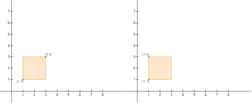
Example 1:
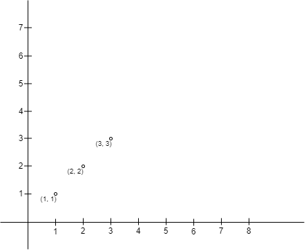
Input: points = [[1,1],[2,2],[3,3]] Output: 0 Explanation: There is no way to place Alice and Bob such that Alice can build a fence with Alice's position as the upper left corner and Bob's position as the lower right corner. Hence we return 0.
Example 2:
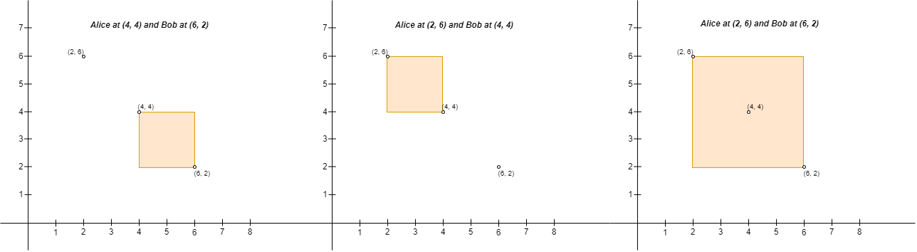
Input: points = [[6,2],[4,4],[2,6]] Output: 2 Explanation: There are two ways to place Alice and Bob such that Alice will not be sad: - Place Alice at (4, 4) and Bob at (6, 2). - Place Alice at (2, 6) and Bob at (4, 4). You cannot place Alice at (2, 6) and Bob at (6, 2) because the person at (4, 4) will be inside the fence.
Example 3:
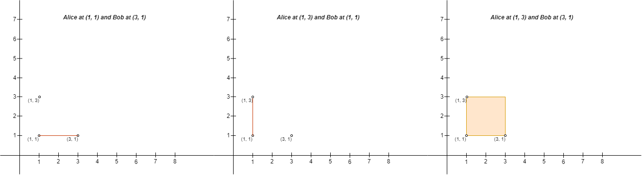
Input: points = [[3,1],[1,3],[1,1]] Output: 2 Explanation: There are two ways to place Alice and Bob such that Alice will not be sad: - Place Alice at (1, 1) and Bob at (3, 1). - Place Alice at (1, 3) and Bob at (1, 1). You cannot place Alice at (1, 3) and Bob at (3, 1) because the person at (1, 1) will be on the fence. Note that it does not matter if the fence encloses any area, the first and second fences in the image are valid.
Constraints:
2 <n <= 1000=points[i].length =2=-10=^{=9}= <= points[i][0], points[i][1] <= 10=9- All
points[i]are distinct.
※ 2.14.8.1. Constraints and Edge Cases
※ 2.14.8.2. My Solution (Code)
※ 2.14.8.2.1. v0: initial, flawed passes half test cases
1: class Solution: 2: │ def numberOfPairs(self, points: List[List[int]]) -> int: 3: │ │ """ 4: │ │ choosing A,B: 5: │ │ A-B rectangle formation is more of consider xa,ya and xb,yb. 6: │ │ As long as xb is not less than xa and yb is not more than ya then it's a legit choice for A,B 7: │ │ 8: │ │ identifying: unhapiness. 9: │ │ consider a sorted array of points (sorted by x then y). 10: │ │ For any two idx i, j where i is for potential placement of A and j is for potential placement of B (assume that works). so let it be xidx, yidx for the point in between. 11: │ │ 12: │ │ anything in the middle must be out of the enclosure. i.e 13: │ │ xidx < xa or xidx > xb or yidx > ya and yidx < yb for it to be legit 14: │ │ 15: │ │ === 16: │ │ 17: │ │ optimising: 18: │ │ if it's sorted and we take two points,then the x value is in between, so we only care about the y values whether they are outside. 19: │ │ """ 20: │ │ points.sort() 21: │ │ n = len(points) 22: │ │ count = 0 23: │ │ placements = set() 24: │ │ 25: │ │ for right in range(1, n): 26: │ │ │ for left in range(right): 27: │ │ │ │ xa,ya = points[left] # alice coords 28: │ │ │ │ xb, yb = points[right] # bob coords 29: │ │ │ │ print(f"xa,ya {xa,ya} | xb,yb {xb,yb}") 30: │ │ │ │ 31: │ │ │ │ if xa == xb and yb > ya: # swap them if possible 32: │ │ │ │ │ xa, ya, xb, yb = xb, yb, xa, ya 33: │ │ │ │ │ print(f"\tswapped, placement:{(xa, ya, xb, yb)}") 34: │ │ │ │ │ 35: │ │ │ │ if xb < xa or yb > ya: # not possible to form enclosure 36: │ │ │ │ │ print("not possible to place A and B: no rect") 37: │ │ │ │ │ continue 38: │ │ │ │ │ 39: │ │ │ │ has_violating_mid_point = any((yb < ymid < ya and xa < xmid < xb) for xmid, ymid in points[left + 1:right]) 40: │ │ │ │ if has_violating_mid_point: 41: │ │ │ │ │ print("\tnot possible to place A and B: unhappy") 42: │ │ │ │ │ continue 43: │ │ │ │ │ 44: │ │ │ │ print(f"adding placement:{(xa, ya, xb, yb)}") 45: │ │ │ │ 46: │ │ │ │ placements.add((xa, ya, xb, yb)) 47: │ │ │ │ 48: │ │ return len(placements)
Problems:
- we check for mid points and compare the y values but after sorting just by x then y (both in ascending direction), points between left and right may still have y values that cause invalid rectangles even if their x is not strictly between xa, xb.
※ 2.14.8.2.2. v1: community provided optimal sweepline algo
1: class Solution: 2: │ def numberOfPairs(self, points: List[List[int]]) -> int: 3: │ │ """ 4: │ │ We use the sweepline algo here, we first sort in ascending x values and descending y values, this allows us to just sweep from left to right. This ensures that when sweeping to the right, no other point has a smaller x for the current region. 5: │ │ 6: │ │ This helps us to implement a simple "mid-point check". 7: │ │ """ 8: │ │ points.sort(key=lambda pt: (pt[0], -pt[1])) 9: │ │ n = len(points) 10: │ │ ans = 0 11: │ │ for i, (xa, ya) in enumerate(points): 12: │ │ │ max_y = float('-inf') 13: │ │ │ for xb, yb in points[i+1:]: 14: │ │ │ │ if yb > ya: # Bob must be strictly below or same row as Alice 15: │ │ │ │ │ continue 16: │ │ │ │ if yb > max_y: 17: │ │ │ │ │ ans += 1 18: │ │ │ │ │ max_y = yb 19: │ │ return ans
The main trick here is that we sort in ascending x and descending y to make it easier to accumulate things.
※ 2.14.8.3. My Approach/Explanation
<briefly explain your reasoning, algorithm, and why you chose it>
※ 2.14.8.4. My Learnings/Questions
- I think this is a good formalisation of the sweepline algo, it has the sort by x and then by negative y approach, somewhat reminiscent of the envelopes kind of question
※ 2.14.8.4.1. Primer on Sweep line algo
Sweep Line Algorithm: A Primer
What is it?
A “sweep line” (or “line sweep”) is a geometric algorithmic technique where you move an imaginary line (often vertical or horizontal) across the input (points, intervals, rectangles, events), processing “events” as the line passes them.
Where is it used?
Intervals/segment intersection (finding overlaps, counting active intervals)
Closest pair of points
Counting/aggregating events by position
Rectangle union/intersection
Area/coverage/overlap calculation in geometry
Main steps
Sort all events by the sweep coordinate (often x).
Process events in order:
Update an ’active set’ (a data structure representing currently relevant objects/intervals as the sweep line passes)
Take required actions for each event (insert, remove, query, aggregate)
Optionally, do a secondary sweep (by y or in reverse) if two-dimensional logic is required.
What to look for when applying it:
There is a natural “order” (often x or time) to events.
For any event, you can efficiently update/query the ’active set’.
The solution to your problem depends on efficiently knowing about or querying the active set at each event (e.g., which segments/points/rectangles are “active” right now).
Data structure for the active set: BST, multiset, interval tree, balanced heap, set, etc. depending on what queries/updates you need.
Cautions and subtleties
Avoid off-by-one errors at event boundaries: define “entry” and “exit” events precisely.
Watch for degenerate/duplicate events (e.g. multiple rectangles starting at the same x).
For multidimensional problems, sometimes requires trickier event handling or a nested/secondary structure (e.g., segment tree for y).
References
※ 2.14.8.5. Prompt for GPT Evaluation
Please do the following:
- Evaluate the correctness of my solution. Are there any logical or edge case errors?
- Analyze the time and space complexity of my code.
- Suggest improvements in code style, efficiency, or clarity.
- Compare my approach to the optimal solution (if different).
- Provide a sample optimal solution (if mine is not optimal).
- Point out any Pythonic (or language-specific) improvements.
Are there any completely different approaches to this problem?
- e.g something that uses a completely different data structure
If so, then help me gain the intuition for it and show the code clearly
- Answer my specific questions (if any are listed above).
※ 2.14.8.6. Prompt for GPT Evaluation (with Greedy)
Please do the following:
- Evaluate the correctness of my solution. Are there any logical or edge case errors?
- Analyze the time and space complexity of my code.
- Suggest improvements in code style, efficiency, or clarity.
- Compare my approach to the optimal solution (if different).
- Provide a sample optimal solution (if mine is not optimal).
- Point out any Pythonic (or language-specific) improvements.
Are there any completely different approaches to this problem?
- e.g something that uses a completely different data structure
If so, then help me gain the intuition for it and show the code clearly
- Answer my specific questions (if any are listed above).
ALso help me evaluate this in the context of greedy algorithms, ensuring that a good framework of presenting this problem into a greedy algo is given / understood.
※ 2.14.8.7. Prompt for GPT Evaluation (with DP)
Please do the following:
- Evaluate the correctness of my solution. Are there any logical or edge case errors?
- Analyze the time and space complexity of my code.
- Suggest improvements in code style, efficiency, or clarity.
- Compare my approach to the optimal solution (if different).
- Provide a sample optimal solution (if mine is not optimal).
- Point out any Pythonic (or language-specific) improvements.
Are there any completely different approaches to this problem?
- e.g something that uses a completely different data structure
If so, then help me gain the intuition for it and show the code clearly
- Answer my specific questions (if any are listed above).
ALso help me evaluate this in the context of greedy algorithms, ensuring that a good framework of presenting this problem into a greedy algo is given / understood.
Additionally, use my notes for Dynamic Programming and use the recipes that are here.
Recipe to define a solution via DP
[Generate Naive Recursive Algo]
Characterise the structure of an optimal solution \(\implies\) what are the subproblems? \(\implies\) are they independent subproblems? \(\implies\) how many subproblems will there be?
- Recursively define the value of an optimal solution \(\implies\) does this have the overlapping sub-problems property? \(\implies\) what’s the cost of making a choice? \(\implies\) how many ways can I make that choice?
- Compute value of an optimal solution
- Construct optimal solution from computed information Defining things
- Optimal Substructure:
A problem exhibits “optimal substructure” if an optimal solution to the problem contains within it optimal solutions to subproblems.
Elements of Dynamic Programming: Key Indicators of Applicability [1] Optimal Sub-Structure Defining “Optimal Substructure” A problem exhibits optimal substructure if an optimal solution to the problem contains within it optimal solutions to sub-problems.
- typically a signal that DP (or Greedy Approaches) will apply here.
- this is something to discover about the problem domain Common Pattern when Discovering Optimal Substructure
solution involves making a choice e.g. choosing an initial cut in the rod or choosing what k should be for splitting the matrix chain up
\(\implies\) making the choice also determines the number of sub-problems that the problem is reduced to
- Assume that the optimal choice can be determined, ignore how first.
- Given the optimal choice, determine what the sub-problems looks like \(\implies\) i.e. characterise the space of the subproblems
- keep the space as simple as possible then expand
typically the substructures vary across problem domains in 2 ways:
[number of subproblems]
how many sub-problems does an optimal solution to the original problem use?
- rod cutting:
# of subproblems = 1(of size n-i) where i is the chosen first cut lengthmatrix split:
# of subproblems = 2(left split and right split)[number of subproblem choices]
how many choices are there when determining which subproblems(s) to use in an optimal solution. i.e. now that we know what to choose, how many ways are there to make that choice?
- rod cutting: # of choices for i = length of first cut,
nchoices- matrix split: # of choices for where to split (idx k) =
j - iNaturally, this is how we analyse the runtime:
# of subproblems * # of choices @ each sub-problem- Reason to yourself if and how solving the subproblems that are used in an optimal solution means that the subproblem-solutions are also optimal. This is typically done via the
cut-and-paste argument.Caveat: Subproblems must be
independent
- “independent subproblems”
- solution to one subproblem doesn’t affect the solution to another subproblem for the same problem
example: Unweighted Shortest Path (independent subproblems) vs Unweighted Longest Simple Path (dependent subproblems)
Consider graph \(G = (V,E)\) with vertices \(u,v \notin V\)
- Unweighted shortest path: we want to find path \(u\overset{p}{\leadsto}v\) then we can break it down into subpaths \(u\overset{p1}{\leadsto}w\overset{p2}{\leadsto}v\) (optimal substructure). If path, p, is optimal from \(u\leadsto{v}\) then p1 must be shortest path from \(u\leadsto{w}\) and likewise p2 must be shortest path from \(w\leadsto{v}\) (cut-and-paste argument) Here, we know that the subproblems are independent.
- Unweighted Longest Simple Path: the subproblems can have paths that overlap (not subproblem overlap), hence it’s not independent because the vertices that appear can appear in the solution to the second subproblem
Terminology: Optimal substruture vs optimal solution optimal substructure is a property that enables efficient computation of the optimal value, while the solution is the specific configuration that yields that optimal value
You’re right that in dynamic programming algorithms for optimization problems, the goal is usually to find an optimal solution rather than the unique optimal solution. Here’s how the optimal substructure and the actual solution differ:
### Optimal Substructure
The optimal substructure refers to the property that the optimal solution to a problem can be constructed from the optimal solutions to its subproblems. This means that if we know the optimal solutions to the subproblems, we can efficiently determine the optimal solution to the overall problem.
For example, in the rod cutting problem, if we know the maximum revenue for rods of length 1 to n-1, we can efficiently determine the maximum revenue for a rod of length n by considering cutting the rod at each possible length and taking the maximum revenue.
### The Solution
The actual solution, on the other hand, refers to the specific configuration or set of choices that yields the optimal value. In the rod cutting problem, the solution would be the specific way to cut the rod that results in the maximum revenue.
The key difference is that the optimal substructure allows us to efficiently compute the optimal value, but it doesn’t necessarily specify the exact solution. There may be multiple solutions that yield the same optimal value.
For example, in the rod cutting problem, there may be multiple ways to cut the rod that result in the same maximum revenue. The optimal substructure allows us to efficiently compute the maximum revenue, but it doesn’t specify which particular cutting configuration to choose.
So in summary, the optimal substructure is a property that enables efficient computation of the optimal value, while the solution is the specific configuration that yields that optimal value. Dynamic programming algorithms leverage the optimal substructure to efficiently compute the optimal value, but the actual solution may not be uniquely determined.
Citations: [1] https://library.fiveable.me/key-terms/programming-for-mathematical-applications/optimal-substructure [2] https://afteracademy.com/blog/optimal-substructure-and-overlapping-subproblems/ [3] https://www.geeksforgeeks.org/optimal-substructure-property-in-dynamic-programming-dp-2/ [4] https://labuladong.gitbook.io/algo-en/i.-dynamic-programming/optimalsubstructure [5] https://stackoverflow.com/questions/33563230/optimal-substructure-in-dynamic-programing [6] https://en.wikipedia.org/wiki/Optimal_substructure [7] https://www.cs.cmu.edu/~15451-f22/lectures/lec09-dp1.pdf [8] https://www.javatpoint.com/optimal-substructure-property
[2] Overlapping Sub-Problems
- DP should be disambiguated from Divide & Conquer:
- for Divide&Conquer, choosing a division point generates brand new problems that likely don’t overlap
- for DP, the space of sub-problems is small and hence if done purely recursively, the same operations get computed multiple times
[Practical point] Reconstructing an optimal solution Since one way to look at DP is table-filling, we typically have:
- table of costs
- table of optimal choices
the table of optimal choices can be built from the table of costs, but we want to avoid recalculating the optimal choices
Memoisation as an alternative
- the textbook used sees this as an alternative and memoised tables as the aux DS for recursive, top-down approaches
- memoisation also exploits the observation that the space of the subproblems is small and hence overlapping
Common Misconceptions Here are some common misconception, based on what perplexity says
Based on the search results, here are some of the common misconceptions that learners have about dynamic programming:
## 1. Misconceptions about the Definition and Purpose of Dynamic Programming
- Thinking that recursion and dynamic programming are explicitly different concepts[3].
- Believing that dynamic programming is exclusively used to solve optimization problems[3].
## 2. Misconceptions about the Optimal Substructure Property
- Assuming that the optimal solution to a problem can be constructed from any combination of optimal solutions to its subproblems, rather than specific optimal solutions to the right subproblems[1][2].
- Thinking that the optimal solution to a problem can be constructed from optimal solutions to unrelated subproblems[4].
## 3. Misconceptions about Memoization and Tabulation
- Failing to recognize that memoization (top-down) and tabulation (bottom-up) are two different implementation strategies for dynamic programming[1][2].
- Believing that memoization always involves recursion and tabulation always involves iteration[1][2].
## 4. Misconceptions about the Filling Order of the DP Table
- Assuming that the DP table must always be filled in a specific order (e.g., always from small to big cases), without understanding that the order depends on the problem’s dependencies and constraints[1][2][4].
## 5. Misconceptions about the Relationship between Subproblems
- Thinking that the solutions to all subproblems are needed to solve the original problem, rather than understanding that only specific optimal solutions to the right subproblems are needed[1][2].
## 6. Misconceptions about the Efficiency of Dynamic Programming
- Believing that dynamic programming always leads to polynomial-time algorithms, without understanding that it can sometimes only slightly improve the exponential-time complexity[4].
Understanding and addressing these common misconceptions can help learners develop a more accurate and comprehensive understanding of dynamic programming and its applications.
Citations: [1] https://dl.acm.org/doi/10.1145/3159450.3159528 [2] https://dl.acm.org/doi/abs/10.1145/3159450.3159528 [3] https://ics.uci.edu/~mikes/papers/Student_Misconceptions_Dynamic_Programming.pdf [4] https://www.cs.cmu.edu/~15451-f22/lectures/lec09-dp1.pdf [5] https://www.reddit.com/r/compsci/comments/er05hn/help_me_wrap_my_head_around_dynamic_programming/ [6] https://yourbasic.org/algorithms/dynamic-programming-explained/ [7] https://stackoverflow.com/questions/33563230/optimal-substructure-in-dynamic-programing [8] https://lec.inf.ethz.ch/DA/2020/slides/daLecture13.en.pdf
Greedy Algos vs DP When comparing greedy strategies and dynamic programming (DP), it’s essential to understand how they differ in methodology, application, and the nature of the problems they solve. Both approaches involve identifying optimal substructures, but they apply this concept in distinct ways. Here’s a detailed disambiguation based on the search results:
### 1. Definition and Approach
- Greedy Strategy:
- A greedy algorithm makes the most optimal choice at each step with the hope that these local optimum choices will lead to a global optimum solution. It does not consider the overall impact of the current choice on future decisions.
- Greedy algorithms are typically simpler and faster to implement, as they do not require storing results of subproblems. However, they do not guarantee an optimal solution for all problems.
- Dynamic Programming:
- Dynamic programming is a technique used to solve complex problems by breaking them down into simpler subproblems. It is based on the principles of optimal substructure and overlapping subproblems.
- DP guarantees an optimal solution by considering all possible cases and storing the results of subproblems to avoid redundant computations. This can lead to higher time and space complexity compared to greedy algorithms.
### 2. Optimal Substructure
- Greedy Algorithms:
- Greedy algorithms rely on the greedy choice property, which means that a locally optimal choice leads to a globally optimal solution. However, this property does not hold for all problems, which is why greedy algorithms may fail to find the optimal solution in some cases.
- Dynamic Programming:
- Dynamic programming explicitly uses the optimal substructure property, where an optimal solution to a problem can be constructed from optimal solutions of its subproblems. DP ensures that all relevant subproblems are considered, leading to a guaranteed optimal solution.
### 3. Subproblem Reuse
- Greedy Strategy:
- Greedy algorithms typically do not reuse solutions to subproblems. Each decision is made independently based on the current state without revisiting previous choices.
- Dynamic Programming:
- DP explicitly solves and caches solutions to overlapping subproblems. This reuse of subproblem solutions is a key feature of dynamic programming, allowing for efficient computation.
### 4. Complexity and Efficiency
- Greedy Algorithms:
- Greedy algorithms are generally more efficient in terms of time complexity due to their straightforward approach. They often run in linear or logarithmic time, depending on the problem.
- They are suitable for problems where local optimization leads to global optimization, such as in minimum spanning trees or certain shortest path problems.
- Dynamic Programming:
- DP can be less efficient than greedy algorithms in terms of time complexity, especially if every possible solution is computed. However, proper use of memoization can mitigate this.
- DP is applicable to problems with overlapping subproblems and optimal substructure, such as the Fibonacci sequence, longest common subsequence, or knapsack problems.
### 5. Examples
- Greedy Algorithms:
- Common examples include:
- Fractional Knapsack Problem: Where you can take fractions of items.
- Minimum Spanning Tree: Algorithms like Prim’s and Kruskal’s.
- Huffman Coding: For optimal prefix codes.
- Dynamic Programming:
- Common examples include:
- 0/1 Knapsack Problem: Where you cannot take fractions of items.
- Longest Common Subsequence: Finding the longest subsequence present in both sequences.
- Matrix Chain Multiplication: Finding the most efficient way to multiply a given sequence of matrices.
### Conclusion
In summary, while both greedy strategies and dynamic programming involve the concept of optimal substructure, they differ significantly in their approach to problem-solving. Greedy algorithms make decisions based on local optimality without revisiting previous choices, whereas dynamic programming systematically considers all possible subproblems and their solutions to ensure a globally optimal result. Understanding these differences allows for better problem-solving strategies and the appropriate application of each method based on the problem’s characteristics.
Citations: [1] https://www.boardinfinity.com/blog/greedy-vs-dp/ [2] https://www.shiksha.com/online-courses/articles/difference-between-greedy-and-dynamic-programming-blogId-158053 [3] https://www.interviewbit.com/blog/difference-between-greedy-and-dynamic-programming/ [4] https://stackoverflow.com/questions/16690249/what-is-the-difference-between-dynamic-programming-and-greedy-approach [5] https://www.geeksforgeeks.org/greedy-approach-vs-dynamic-programming/ [6] https://byjus.com/gate/difference-between-greedy-approach-and-dynamic-programming/ [7] https://www.cs.cmu.edu/~15451-f22/lectures/lec09-dp1.pdf [8] https://ics.uci.edu/~mikes/papers/Student_Misconceptions_Dynamic_Programming.pdf
General Takeaways Bottom-up vs Top-Down
- we can use a subproblem graph to show the relationship with the subproblems ==> diff b/w bottom up and top-down is how these deps are handled (recursive-called or soundly iterated with a proper direction)
- aysymptotic runtime is pretty similar since both solve similar \(\Omega(n^{2})\)
- Bottom up:
- basically considers order at which the subproblems are solved
- because of the ordered way of solving the smaller sub-problems first, there’s no need for recursive calls and code can be iterative entirely
- so no overhead from function calls
- no chance of stack overflow
- benefits from data-locality
- a way to see the vertices of the subproblem graph such that the subproblems y-adjacent to a given subproblem x is solved before subproblem x is solved
※ 2.14.8.8. [Optional] Additional Context
<e.g., “I struggled with X”, “I want to know about alternative algorithms”, etc.>
※ 2.15. Greedy Algos
| Headline | Time | ||
|---|---|---|---|
| Total time | 5:23 | ||
| Greedy Algos | 5:23 | ||
| [111] Maximum Subarray (53) | 0:33 | ||
| [112] Jump Game (55) | 0:18 | ||
| [113] Jump Game II (45) | 0:18 | ||
| [114] Gas Station (134) | 1:08 | ||
| [115] Hand of Straights (846) | 0:29 | ||
| [116] Merge Triplets to Form Target… | 1:16 | ||
| [117] Partition Labels (763) | 0:54 | ||
| [118] Valid Parenthesis String (678) | 0:27 |
※ 2.15.2. [111] Maximum Subarray (53) greedy kadane_algorithm
Given an integer array nums, find the subarray with the largest sum,
and return its sum.
Example 1:
Input: nums = [-2,1,-3,4,-1,2,1,-5,4] Output: 6 Explanation: The subarray [4,-1,2,1] has the largest sum 6.
Example 2:
Input: nums = [1] Output: 1 Explanation: The subarray [1] has the largest sum 1.
Example 3:
Input: nums = [5,4,-1,7,8] Output: 23 Explanation: The subarray [5,4,-1,7,8] has the largest sum 23.
Constraints:
1 <nums.length <= 10=5-10=^{=4}= <= nums[i] <= 10=4
Follow up: If you have figured out the O(n) solution, try coding
another solution using the divide and conquer approach, which is more
subtle.
※ 2.15.2.1. Constraints and Edge Cases
Nothing fancy to take note of.
All negative numbers as an edge case
Single element arrays as an edge case
Mixed positives and negatives
※ 2.15.2.2. My Solution (Code)
※ 2.15.2.2.1. v1: correct, working optimal implementation
1: class Solution: 2: │ def maxSubArray(self, nums: List[int]) -> int: 3: │ │ best = -float('inf') 4: │ │ curr_accum = 0 5: │ │ for num in nums: 6: │ │ │ # greedy choice: I make the best choice possible 7: │ │ │ new_accum = curr_accum + num 8: │ │ │ best = max(best, new_accum) 9: │ │ │ # choose A: start from scratch or B: carry on 10: │ │ │ curr_accum = 0 if new_accum < 0 else new_accum 11: │ │ │ 12: │ │ return best
- Complexity Analysis:
- Time: \(O(n)\) — you traverse the array once.
- Space: \(O(1)\) — a fixed number of variables tracked.
- Intent:
for each element, I have 2 choices:
A: I include this element into the final subsequence that gives the max sum
B: or exclude from the final subsequence that gives the max sum
B is taken if I know that inclusion will be the worst for me. Restarting the sum from 0 would be better than including in a value that would make my newly accumulated value negative.
This can proven via a “cut and paste” argument also. Suppose there was a number that was huge that’s to the right of my candidate. And my candidate is an arbitrary negative number. If I include my candidate and the partial sum with the candidate < 0, then it diminishes the effect of my huge positive number. If I choose to start from scratch, then there’s no such diminishing. Therefore, it’s better to start from scratch in that situation.
I think this is what the greedy choice property is.
The problem then gets reduced to an almost identical sub-problem.
Greedy choice property:
If I take the best decision now (i.e. to include or exclude into the max subseq)
※ 2.15.2.2.2. v2: Cleaned up version:
this is a cleaned up version:
1: class Solution: 2: │ def maxSubArray(self, nums: List[int]) -> int: 3: │ │ best = nums[0] 4: │ │ curr_accum = 0 5: │ │ 6: │ │ for num in nums: 7: │ │ │ curr_accum += num 8: │ │ │ best = max(best, curr_accum) 9: │ │ │ 10: │ │ │ # If curr_accum drops below zero, start fresh 11: │ │ │ if curr_accum < 0: 12: │ │ │ │ curr_accum = 0 13: │ │ │ │ 14: │ │ return best
Improvements:
- Initializing
bestwithnumsensures immediate correctness even when all inputs are negative.
※ 2.15.2.2.3. v3: correct, slower, alternative divide & conquer strategy
Divide and Conquer:
Split array into two halves, recursively find max subarray sum on left, right, and crossing the middle.
The divide and conquer approach to the Maximum Subarray problem reduces the problem into three parts for a given range [left, right] in the array:
- The maximum subarray is entirely in the left half.
- The maximum subarray is entirely in the right half.
- The maximum subarray crosses the middle point.
We recursively find each part and return the maximum.
1: from typing import List 2: 3: class Solution: 4: │ def maxSubArray(self, nums: List[int]) -> int: 5: │ │ def helper(left: int, right: int) -> int: 6: │ │ │ # Base case: single element 7: │ │ │ if left == right: 8: │ │ │ │ return nums[left] 9: │ │ │ │ 10: │ │ │ mid = left + (right - left) // 2 11: │ │ │ 12: │ │ │ # Maximum subarray in left half 13: │ │ │ left_max = helper(left, mid) 14: │ │ │ 15: │ │ │ # Maximum subarray in right half 16: │ │ │ right_max = helper(mid + 1, right) 17: │ │ │ 18: │ │ │ # Maximum subarray crossing mid 19: │ │ │ cross_max = max_crossing_subarray(left, mid, right) 20: │ │ │ 21: │ │ │ # Return overall max 22: │ │ │ return max(left_max, right_max, cross_max) 23: │ │ │ 24: │ │ def max_crossing_subarray(left: int, mid: int, right: int) -> int: 25: │ │ │ # Find max subarray sum crossing mid, including mid 26: │ │ │ 27: │ │ │ left_sum = float('-inf') 28: │ │ │ curr_sum = 0 29: │ │ │ for i in range(mid, left - 1, -1): 30: │ │ │ │ curr_sum += nums[i] 31: │ │ │ │ if curr_sum > left_sum: 32: │ │ │ │ │ left_sum = curr_sum 33: │ │ │ │ │ 34: │ │ │ right_sum = float('-inf') 35: │ │ │ curr_sum = 0 36: │ │ │ for i in range(mid + 1, right + 1): 37: │ │ │ │ curr_sum += nums[i] 38: │ │ │ │ if curr_sum > right_sum: 39: │ │ │ │ │ right_sum = curr_sum 40: │ │ │ │ │ 41: │ │ │ return left_sum + right_sum 42: │ │ │ 43: │ │ return helper(0, len(nums) - 1)
Time Complexity:
- Recurrence: \[T(n) = 2T(n/2) + O(n)\] → by Master theorem, \[O(n \log n)\]
※ 2.15.2.3. My Approach/Explanation
This is the classic kadane’s algo.
If I were to think of it as a greedy approach
※ 2.15.2.4. My Learnings/Questions
- Improvements :
- we can init the
bestto be the first value in thenumsarray, which makes it easy to handle the negative number cases as well. This is what the cleaned up version does.
- we can init the
- The approach works even with all negatives because you initialize best = -inf and update before resetting.
- Kadane’s Algorithm: A Greedy Framework Explanation
- Framework to understand and apply greedy algorithms:
- Problem interpretation:
- Goal: maximize sum of a contiguous subarray.
- For each element, decide whether to extend existing subarray or start new.
- Greedy Choice Property:
- If current accumulated sum is negative, it will only reduce the sum of any future subarray.
- The best choice is to drop the current subarray and start fresh at the next element.
- This is a locally optimal choice leading to global optimum.
- Optimal Substructure:
- Maximum subarray ending at i depends on max subarray ending at i-1.
- If extending the subarray ending at i-1 leads to negative sum, reset.
- Algorithm:
- For each num:
- Update running sum: currsum = max(num, currsum + num)
- Track max sum as you move forward.
- Proof (Intuition):
- Including negative partial sums can never lead to a better larger sum; beginning anew is always better.
- Problem interpretation:
- Applying this to your solution
- At each iteration, you make a greedy decision:
- Continue to accumulate if it benefits (currsum + num >= num), otherwise start new subarray.
- This reduces the problem into deciding between:
- A: Extend old subarray.
- B: Begin new subarray at the current element.
- These local optimal choices sum to global optimum.
- At each iteration, you make a greedy decision:
- Framework to understand and apply greedy algorithms:
※ 2.15.2.5. [Optional] Additional Context
I think I have an intuition for the Kadane’s algorithm. Happy with myself.
※ 2.15.3. [112] Jump Game (55) greedy
You are given an integer array nums. You are initially positioned at
the array’s first index, and each element in the array represents your
maximum jump length at that position.
Return true if you can reach the last index, or false otherwise.
Example 1:
Input: nums = [2,3,1,1,4] Output: true Explanation: Jump 1 step from index 0 to 1, then 3 steps to the last index.
Example 2:
Input: nums = [3,2,1,0,4] Output: false Explanation: You will always arrive at index 3 no matter what. Its maximum jump length is 0, which makes it impossible to reach the last index.
Constraints:
1 <nums.length <= 10=40 <nums[i] <= 10=5
※ 2.15.3.1. Constraints and Edge Cases
<list constraints, input limits, or tricky edge cases here>
※ 2.15.3.2. My Solution (Code)
※ 2.15.3.2.1. v0: wrong, complicated version
1: class Solution: 2: │ def canJump(self, nums: List[int]) -> bool: 3: │ │ if not nums or (len(nums) == 1 and nums[0] != 0): 4: │ │ │ return True 5: │ │ │ 6: │ │ n = len(nums) 7: │ │ i = n - 2 8: │ │ while not_source_found:=not(((n - 1) - (n-i) == nums[i])): 9: │ │ │ if i == 0: 10: │ │ │ │ return False 11: │ │ │ i -= 1 12: │ │ │ 13: │ │ return self.canJump(nums[:i + 1])
- the slicing here will create new string copies and this will make things really efficient.
- the not source probably has an okay but convoluted logic behind it.
※ 2.15.3.2.2. v1: correct guided approach
1: class Solution: 2: │ def canJump(self, nums: List[int]) -> bool: 3: │ │ goal = len(nums) - 1 4: │ │ 5: │ │ # start from left of the goal 6: │ │ for i in range(len(nums) - 2, -1, -1): 7: │ │ │ # if I can find a jmp source, I take it: 8: │ │ │ if i + nums[i] >= goal: 9: │ │ │ │ goal = i 10: │ │ │ │ 11: │ │ return goal == 0 12:
The improvement here is that the logic is a little clearer. The greedy choice of “pick the first jump source I can get” should work right.
For the case where it’s not possible to jump, it’s because the goal could never reach 0.
This is a standard optimal greedy approach, working as follows:
You track the target (goal) index you want to reach (initially the last index).
From right to left, if the current index i can jump at least to the goal, update the goal to i.
If at the end goal is 0, you can reach the last index from start.
This is correct and passes all test cases.
this is a cleaned up and annotated version by the bot:
1: class Solution: 2: │ def canJump(self, nums: List[int]) -> bool: 3: │ │ # The leftmost position that can reach the end (initially the last index) 4: │ │ leftmost_reachable = len(nums) - 1 5: │ │ 6: │ │ # Traverse from right to left 7: │ │ for i in range(len(nums) - 2, -1, -1): 8: │ │ │ # If current position can jump to or beyond leftmost_reachable, update leftmost_reachable 9: │ │ │ if i + nums[i] >= leftmost_reachable: 10: │ │ │ │ leftmost_reachable = i 11: │ │ │ │ 12: │ │ # If leftmost_reachable is 0, start can reach the end 13: │ │ return leftmost_reachable == 0
※ 2.15.3.3. My Approach/Explanation
I need to take the BEST optimal local action to give me a globally optimal action.
THis DOES NOT mean that I need to find the biggest jump source (since I’m not trying to minimise my jumps, I’m just trying to jump and get where I want to get). Therefore, I can make the choice to jump as soon as I have a viable candidate.
※ 2.15.3.4. My Learnings/Questions
- I think the improved logic is a lot clearer.
- Alternative approaches:
- Backtracking / DFS:
- Try all jumps from the current position — exponential time, impractical.
- Dynamic Programming:
- Memoize whether each index can reach the end — yields \(O(n^2)\) in worst case, less efficient.
- Your greedy method is preferred for linear time.
- Backtracking / DFS:
- Intuition and Framework for Greedy Approach
- Framework for Greedy Algorithms
- Problem Restatement:
- Can I get from the start of an array to the last index by making jumps limited by the value at each index?
- Greedy Choice:
- From the right side, greedily determine the earliest index (from the POV of the goal, first index that we encounter) that can reach the end or a previously known reachable index.
- Optimal Substructure:
- If position i can reach some position that can reach the end, then i itself can reach the end.
- Local Decision:
- If you can jump from i past or onto a “goal”, update the goal to i.
- Global Optimum:
- If the goal is moved all the way to index 0, the answer is true.
- Problem Restatement:
- Why does this work?
- Instead of trying all jump possibilities forward (complex), work backwards avoiding repeated work.
- At each step, you greedily mark positions that make progress towards the end (moving the goal index to the far left).
- Eventually, either the start index can reach the goal (which would be index 0), or it cannot.
- The local greedy choices result in the correct global solution because the problem has an optimal substructure (reachable states depend on previously reachable states).
- Framework for Greedy Algorithms
※ 2.15.4. [113] Jump Game II (45) greedy rephrase_the_question
You are given a 0-indexed array of integers nums of length n. You
are initially positioned at nums[0].
Each element nums[i] represents the maximum length of a forward jump
from index i. In other words, if you are at nums[i], you can jump to
any nums[i + j] where:
0 <j <= nums[i]= andi + j < n
Return the minimum number of jumps to reach nums[n - 1]. The test
cases are generated such that you can reach nums[n - 1].
Example 1:
Input: nums = [2,3,1,1,4] Output: 2 Explanation: The minimum number of jumps to reach the last index is 2. Jump 1 step from index 0 to 1, then 3 steps to the last index.
Example 2:
Input: nums = [2,3,0,1,4] Output: 2
Constraints:
1 <nums.length <= 10=40 <nums[i] <= 1000=- It’s guaranteed that you can reach
nums[n - 1].
※ 2.15.4.1. Constraints and Edge Cases
<list constraints, input limits, or tricky edge cases here>
※ 2.15.4.2. My Solution (Code)
※ 2.15.4.2.1. v0 [wrong] likely wrong greedy choice
1: class Solution: 2: │ def jump(self, nums: List[int]) -> int: 3: │ │ # trivial base case: 4: │ │ if len(nums) == 1: 5: │ │ │ return 0 6: │ │ │ 7: │ │ idx = 0 8: │ │ count = 0 9: │ │ while idx < len(nums): 10: │ │ │ max_jump = nums[idx] 11: │ │ │ rightmost_idx = idx + max_jump 12: │ │ │ if idx < len(nums) and rightmost_idx >= len(nums) - 1: 13: │ │ │ │ count += 1 14: │ │ │ │ break 15: │ │ │ │ 16: │ │ │ best_candidate_idx = idx 17: │ │ │ best_candidate_val = -float('inf') 18: │ │ │ for candidate_idx in range(idx, rightmost_idx + 1): 19: │ │ │ │ candidate = nums[candidate_idx] 20: │ │ │ │ if candidate >= best_candidate_val: 21: │ │ │ │ │ best_candidate_val = candidate 22: │ │ │ │ │ best_candidate_idx = candidate_idx 23: │ │ │ │ │ 24: │ │ │ idx += nums[best_candidate_idx] 25: │ │ │ count += 1 26: │ │ │ 27: │ │ return count 28:
this attempts to jump based on best choice .
This doesn’t ensure that we get the best choice in terms of what we are trying to achieve.
We are trying to make sure that we have the least jumps. This means at each local choice, I need to choose something that gives me the rightmost advancement.
This approach doesn’t consider the rightmost advancement correctly.
※ 2.15.4.2.2. v1 [correct] correct greedy choice
1: class Solution: 2: │ def jump(self, nums: List[int]) -> int: 3: │ │ # trivial base case: 4: │ │ if len(nums) == 1: 5: │ │ │ return 0 6: │ │ │ 7: │ │ idx = 0 8: │ │ count = 0 9: │ │ while idx < len(nums): 10: │ │ │ max_reachable_idx = idx + nums[idx] 11: │ │ │ next_idx = idx 12: │ │ │ furthest_reach = 0 13: │ │ │ for candidate_idx in range(idx, max_reachable_idx + 1): 14: │ │ │ │ if candidate_idx >= len(nums) - 1: 15: │ │ │ │ │ return count + 1 16: │ │ │ │ │ 17: │ │ │ │ final_place = candidate_idx + nums[candidate_idx] 18: │ │ │ │ if final_place > furthest_reach: 19: │ │ │ │ │ furthest_reach = final_place 20: │ │ │ │ │ next_idx = candidate_idx 21: │ │ │ │ │ 22: │ │ │ count += 1 23: │ │ │ idx = next_idx 24: │ │ │ 25: │ │ return count
Your v1 solution:
Iteratively from idx, look at all reachable positions (idx + nums[idx]).
From these, pick the position candidateidx whose candidateidx + nums[candidateidx] (furthest reachable from next step) is maximum.
Jump there and increment jump count.
If during scanning reachable candidates you find anyone can jump directly to or beyond the last index, return count + 1.
Else keep looping.
This is correct and standard greedy to minimize jumps, as it always picks the next jump that leads to the overall furthest reachable index.
Analysis is Amortized: Nested loop could look \(O(n^{2})\) in worst case if jump lengths are very small.
But since you progress through the array by making jumps, and the inner loop only scans reachable positions from the current idx, the amortized complexity is still \(O(n)\).
Space is \(O(1)\), only a few variables.
To refactor this to be more similar to the canonical optimal:
1: class Solution: 2: │ def jump(self, nums: List[int]) -> int: 3: │ │ if len(nums) == 1: 4: │ │ │ return 0 5: │ │ │ 6: │ │ jumps = 0 7: │ │ current_end = 0 # boundary of current jump coverage 8: │ │ furthest = 0 # furthest reachable index in next jump 9: │ │ 10: │ │ for i in range(len(nums) - 1): # no need to jump from last index 11: │ │ │ furthest = max(furthest, i + nums[i]) 12: │ │ │ 13: │ │ │ # When we reach end of current jump coverage, we "make the jump" 14: │ │ │ if i == current_end: 15: │ │ │ │ jumps += 1 16: │ │ │ │ current_end = furthest 17: │ │ │ │ 18: │ │ │ │ if current_end >= len(nums) - 1: 19: │ │ │ │ │ break 20: │ │ │ │ │ 21: │ │ return jumps
I see this as a sweep search pointer then a decision / jump pointer.
※ 2.15.4.2.3. v2: canonical optimal
1: class Solution: 2: │ def jump(self, nums: List[int]) -> int: 3: │ │ if len(nums) == 1: 4: │ │ │ return 0 5: │ │ │ 6: │ │ jumps = 0 7: │ │ current_end = 0 # End of current jump coverage 8: │ │ furthest = 0 # Furthest reachable index so far 9: │ │ 10: │ │ for i in range(len(nums) - 1): # no need to jump from last element 11: │ │ │ furthest = max(furthest, i + nums[i]) 12: │ │ │ 13: │ │ │ # When reach the boundary of current jump range 14: │ │ │ if i == current_end: 15: │ │ │ │ jumps += 1 16: │ │ │ │ current_end = furthest 17: │ │ │ │ 18: │ │ │ │ if current_end >= len(nums) - 1: 19: │ │ │ │ │ break 20: │ │ │ │ │ 21: │ │ return jumps
How this works:
For each index i, update how far we can reach (furthest).
When i reaches currentend (end of last jump’s coverage), we must make another jump, so increment jumps and set new currentend as furthest.
When currentend surpasses the last index, we stop.
※ 2.15.4.3. My Approach/Explanation
From the candidates we have from now, we need to make the best choice possible.
How to determine best choice? It brings us the furthest. That’s why I need to consider each candidate amongst my list of options, then consider the max idx I can reach if I were to pick that candidate.
Then I just pick the candidate that gives me the biggest reachability.
※ 2.15.4.4. My Learnings/Questions
Intuition:
the clever part about this is that we need to think about the main goal and think about proxy ways that the goal can be rephrased. In this case, the main goal is to be able to make the least jumps and reach the end. A rephrasing means that we need each jump to make the furthest future progress as possible.
for the canonical optimal solution,
I see this as a sweep search pointer then a decision / jump pointer.
- alternatives
- Dynamic Programming:
- Compute minimum jumps to reach each index, \(O(n^2)\), too slow for large inputs.
- BFS-like traversal:
- Model positions as graph nodes and edges as jumps, use BFS for minimum steps, inefficient compared to greedy.
- The greedy approach is best due to problem structure and constraints.
- Dynamic Programming:
- applying the greedy framework:
- Problem Restatement:
- Find minimum number of jumps to reach the last index.
- Greedy Choice Property:
- At every jump, pick next index from reachable positions that allows furthest future progress.
- Optimal Substructure:
- If minimum jumps to index i is known, then the jumps to reachable next indices from i can be minimized greedily.
- Decision Making:
- Instead of exploring all paths, keep track of max reachable index within current jump; when you reach current jump boundary, increment jump count, update boundary to furthest reachable.
- Global Optimal:
- Greedy steps collectively ensure minimal jumps since you never miss an opportunity to jump to a position enabling maximal progress.
- Problem Restatement:
※ 2.15.4.5. [Optional] Additional Context
Okay this is great, I managed to do it myself and somewhat intuited the correct steps for the greedy thinking. Pats on the back.
※ 2.15.5. [114] Gas Station (134) redo greedy kadane_algorithm
There are n gas stations along a circular route, where the amount of
gas at the i=^{=th} station is gas[i].
You have a car with an unlimited gas tank and it costs cost[i] of gas
to travel from the i=^{=th} station to its next (i + 1)=^{=th}
station. You begin the journey with an empty tank at one of the gas
stations.
Given two integer arrays gas and cost, return the starting gas
station’s index if you can travel around the circuit once in the
clockwise direction, otherwise return -1. If there exists a solution,
it is guaranteed to be unique.
Example 1:
Input: gas = [1,2,3,4,5], cost = [3,4,5,1,2] Output: 3 Explanation: Start at station 3 (index 3) and fill up with 4 unit of gas. Your tank = 0 + 4 = 4 Travel to station 4. Your tank = 4 - 1 + 5 = 8 Travel to station 0. Your tank = 8 - 2 + 1 = 7 Travel to station 1. Your tank = 7 - 3 + 2 = 6 Travel to station 2. Your tank = 6 - 4 + 3 = 5 Travel to station 3. The cost is 5. Your gas is just enough to travel back to station 3. Therefore, return 3 as the starting index.
Example 2:
Input: gas = [2,3,4], cost = [3,4,3] Output: -1 Explanation: You can't start at station 0 or 1, as there is not enough gas to travel to the next station. Let's start at station 2 and fill up with 4 unit of gas. Your tank = 0 + 4 = 4 Travel to station 0. Your tank = 4 - 3 + 2 = 3 Travel to station 1. Your tank = 3 - 3 + 3 = 3 You cannot travel back to station 2, as it requires 4 unit of gas but you only have 3. Therefore, you can't travel around the circuit once no matter where you start.
Constraints:
n =gas.length= cost.length1 <n <= 10=50 <gas[i], cost[i] <= 10=4- The input is generated such that the answer is unique.
※ 2.15.5.1. Constraints and Edge Cases
<list constraints, input limits, or tricky edge cases here>
※ 2.15.5.2. My Solution (Code)
※ 2.15.5.2.1. v0 failed attempt
I can’t seem to find out what the substructure really is.
In this attempt, I just try to linear search and find the start gas station. If I find one where I can have the most leftover at the end of it.
Maybe the better approach would have been to work backwards and see if there’s doable n-1 station that will be the min of the doables. This would allow the max diffs to be avaiable for previous journeys.
1: class Solution: 2: │ def canCompleteCircuit(self, gas: List[int], cost: List[int]) -> int: 3: │ │ # init with first gas: 4: │ │ most_leftover = [-1, -1] 5: │ │ 6: │ │ for idx in range(len(gas)): 7: │ │ │ leftover = gas[idx] - cost[idx] 8: │ │ │ if leftover > 0 and leftover > most_leftover[1]: 9: │ │ │ │ most_leftover = [idx, leftover] 10: │ │ │ │ 11: │ │ return most_leftover[0] 12:
- Problem:
- You’re only considering the leftover gas after leaving one station, NOT after completing the entire circuit from idx and returning to idx by passing through all stations.
- Why doesn’t this work?
- The station with the most leftover after the first hop is not always a feasible starting point for the whole journey. You must be able to keep a non-negative balance at every station in the cycle starting from your candidate.
1: class Solution: 2: │ def canCompleteCircuit(self, gas: List[int], cost: List[int]) -> int: 3: │ │ # init with first gas: 4: │ │ most_balance = [None, -float('inf')] 5: │ │ 6: │ │ for idx in range(len(gas)): 7: │ │ │ next_idx = (idx + 1) % len(gas) - 1 8: │ │ │ balance = (gas[idx] + gas[next_idx]) - cost[idx] 9: │ │ │ if balance > 0 and balance > most_balance[1]: 10: │ │ │ │ most_balance = [idx, balance] 11: │ │ │ │ 12: │ │ return most_balance[0]
- Problem:
- This seems to be a miscalculation: you’re summing gas from two stations then subtracting the cost for only one hop, which is not aligned to the problem’s requirement.
- Why doesn’t this work?
- The journey must simulate moving around the entire circle, not just from two stations, or use the first two gas entries.
※ 2.15.5.2.2. v1: [correct, unacceptable] brute force version
this be the brute force version, just putting it in here
1: class Solution: 2: │ def canCompleteCircuit(self, gas: List[int], cost: List[int]) -> int: 3: │ │ for candidate_idx in range(len(gas)): 4: │ │ │ tank = 0 5: │ │ │ found = True 6: │ │ │ for step in range(len(gas)): 7: │ │ │ │ i = (candidate_idx + step) % (len(gas)) 8: │ │ │ │ tank += (gas[i] - cost[i]) 9: │ │ │ │ if tank < 0: 10: │ │ │ │ │ found = False 11: │ │ │ │ │ break 12: │ │ │ if found: 13: │ │ │ │ return candidate_idx 14: │ │ │ │ 15: │ │ return -1
The realisation here is that instead of just starting with the next candidate index like that, we should shift as far up as possible. This is because from candidate_idx to he failing idx everything will not be feasible.
※ 2.15.5.2.3. v2: [correct, optimal greedy] single sweep “kadane-like”
1: class Solution: 2: │ def canCompleteCircuit(self, gas: List[int], cost: List[int]) -> int: 3: │ │ # total_balance: we're just accumulating for all the gas stations, if the total_balance at the end of the accumulation is negative then the journey is impossible. 4: │ │ # curr_balance is just a curr accumulator 5: │ │ total_balance, curr_balance = 0, 0 6: │ │ # best candidate yet (may not be useful if the journey is impossible) 7: │ │ best_start = 0 8: │ │ 9: │ │ for i in range(len(gas)): 10: │ │ │ diff = gas[i] - cost[i] 11: │ │ │ total_balance += diff 12: │ │ │ curr_balance += diff 13: │ │ │ 14: │ │ │ # if impossible then all from best_start to i are impossible, so we restart the joruney from the next one (though we don't actually make the journey) 15: │ │ │ if curr_balance < 0: 16: │ │ │ │ best_start = i + 1 17: │ │ │ │ curr_balance = 0 18: │ │ │ │ 19: │ │ return best_start if total_balance >= 0 else -1
Some pointers:
- The journey can be broken down into “segments of failure” — each time your tank drops below zero, you must restart after that position.
- we don’t need to simulate the whole journey each time, else it will become the brute force solution. We aren’t simulating journeys, at each step, we:
- check if I can have a better start index
- check if I the global journey is even possible
- if it is, then I just pick the best start index I could find
- if it isn’t then I just return the sentinel.
Here’s a slightly more annotated version:
1: class Solution: 2: │ def canCompleteCircuit(self, gas: List[int], cost: List[int]) -> int: 3: │ │ total_tank = 0 # net gas over the whole journey 4: │ │ current_tank = 0 # net gas from the current starting candidate 5: │ │ start_index = 0 # candidate starting point 6: │ │ 7: │ │ for i in range(len(gas)): 8: │ │ │ gain = gas[i] - cost[i] 9: │ │ │ total_tank += gain 10: │ │ │ current_tank += gain 11: │ │ │ 12: │ │ │ # If we can't reach the next station, start from i + 1 13: │ │ │ if current_tank < 0: 14: │ │ │ │ start_index = i + 1 15: │ │ │ │ current_tank = 0 16: │ │ │ │ 17: │ │ return start_index if total_tank >= 0 else -1
※ 2.15.5.3. My Approach/Explanation
I needed to be guided for this.
Initial flawed approach was that “I have to find the best choice I can make”.
What I should have thought of was: “what does it mean to complete the journey? ”
To which the answer is to be able to have a non-negative tank throughout the journey.
So the choice to be made is “should I start here or not”.
For any arbitrary i that is our starting point, if at any future point j, the tank is less than 0, than i can’t be the starting point. We pick a new candidate then.
The key idea here is that we don’t need to simulate the whole journey.
※ 2.15.5.4. My Learnings/Questions
- Any simulation/brute force is suboptimal (\(O(n^2)\)) and can’t pass large cases.
- We have to be patient when exploring the greedy property.
what does it mean to be able to move around the entire circuit?
sum(gas[i] - cost[i] for i in range(len(n))) >0=\(\implies\) we need to keep an eye on the global balance, it should be positive else the journey is NOT possible
If a tank drops below zero, reset start to the next idx from whatever we explored so far.
- Absolutely! Greedy solutions often come from understanding where local choices can safely lead to global correctness. For Gas Station, the reset-point-after-failure property is key.
- General Greedy Problem-solving Steps:
- Formulate the subproblem:
- Can I make a locally optimal decision (e.g., when to reset my starting point) that leads to the global optimum (successful circuit)?
- Greedy choice property:
- If I fail at
curr_balance < 0, any previous candidate in this segment can’t be the start—reset is safe.
- If I fail at
- Optimal substructure:
- Once you fail, the next possible successful start is strictly after your failure point.
- Iterate with this rule:
- Reset candidate each time running tank falls negative, while maintaining total balance.
- Check feasibility:
- Only possible if
total gas ≥ total cost.
- Only possible if
- Formulate the subproblem:
※ 2.15.5.5. [Optional] Additional Context
It ended up being kadane-like
※ 2.15.6. [115] Hand of Straights (846) almost greedy frequency_counting
Alice has some number of cards and she wants to rearrange the cards into
groups so that each group is of size groupSize, and consists of
groupSize consecutive cards.
Given an integer array hand where hand[i] is the value written on
the i=^{=th} card and an integer groupSize, return true if she can
rearrange the cards, or false otherwise.
Example 1:
Input: hand = [1,2,3,6,2,3,4,7,8], groupSize = 3 Output: true Explanation: Alice's hand can be rearranged as [1,2,3],[2,3,4],[6,7,8]
Example 2:
Input: hand = [1,2,3,4,5], groupSize = 4 Output: false Explanation: Alice's hand can not be rearranged into groups of 4.
Constraints:
1 <hand.length <= 10=40 <hand[i] <= 10=91 <groupSize <= hand.length=
Note: This question is the same as 1296: https://leetcode.com/problems/divide-array-in-sets-of-k-consecutive-numbers/
※ 2.15.6.1. Constraints and Edge Cases
- we should pay attention to:
- the meaning of “consecutive” numbers property and what other proprties that it implies
※ 2.15.6.2. My Solution (Code)
※ 2.15.6.2.1. v0: working naive approach
1: import heapq 2: 3: class Solution: 4: │ def isNStraightHand(self, hand: List[int], groupSize: int) -> bool: 5: │ │ # early returns if I can't form groups 6: │ │ if len(hand) % groupSize != 0: 7: │ │ │ return False 8: │ │ │ 9: │ │ num_groups = len(hand) // groupSize 10: │ │ heapq.heapify(hand) 11: │ │ 12: │ │ for group_idx in range(num_groups): 13: │ │ │ return_pile = [] 14: │ │ │ curr_group = [] 15: │ │ │ 16: │ │ │ # use up the hand: 17: │ │ │ while len(curr_group) < groupSize and hand: 18: │ │ │ │ card = heapq.heappop(hand) 19: │ │ │ │ 20: │ │ │ │ if curr_group and card == curr_group[-1] : 21: │ │ │ │ │ # return pile will always be sorted as well. 22: │ │ │ │ │ return_pile.append(card) 23: │ │ │ │ │ 24: │ │ │ │ # has to be consecutive 25: │ │ │ │ elif curr_group and card != curr_group[-1] + 1: 26: │ │ │ │ │ return False 27: │ │ │ │ else: 28: │ │ │ │ │ curr_group.append(card) 29: │ │ │ │ │ 30: │ │ │ if not len(curr_group) == groupSize: 31: │ │ │ │ return False 32: │ │ │ else: 33: │ │ │ │ hand.extend(return_pile) 34: │ │ │ │ heapq.heapify(hand) 35: │ │ │ │ 36: │ │ return True
Your approach:
Checks divisibility of hand size by groupSize early on—good.
Uses a min-heap to always extract the smallest card.
For each group, tries to form a consecutive sequence by popping from the heap.
If a duplicate card is encountered immediately after the current card in the forming group, you put it in a return pile to be reinserted (to be used in another group).
If the next popped card is not consecutive, you return False.
After forming each group, returns cards in the return pile back to the heap and heapifies again.
Heap operations: Each card is pushed/popped multiple times potentially, worst-case up to \(O(n log n)\) heap operations per group.
Since you heapify repeatedly inside the loop, this can degrade to \(O(n^2 log n)\) in the worst case.
Space: \(O(n)\) for heap and additional returnpile list(s).
This works mostly in principle, but it introduces inefficiency and complexity by pushing duplicates back into the heap and re-heapifying many times. Also, the logic with returnpile may cause overhead and might be prone to subtle bugs for edge cases with many duplicates.
This is how we can shape it into the optimal method:
- Avoid re-heapifying inside the loop multiple times; instead, process the hand in a single pass.
- Use a frequency map (collections.Counter) instead of a heap to track counts of cards.
- Iterate cards in ascending order (sorted keys from the counter) and subtract frequencies greedily.
This method naturally fits the greedy approach:
/*always try to form groups starting from the smallest available card.* /
※ 2.15.6.2.2. v1: optimal correct
1: 2: from collections import Counter 3: 4: class Solution: 5: │ def isNStraightHand(self, hand: List[int], groupSize: int) -> bool: 6: │ │ 7: │ │ # early returns if nondivisible 8: │ │ if len(hand) % groupSize != 0: 9: │ │ │ return False 10: │ │ │ 11: │ │ count = Counter(hand) 12: │ │ 13: │ │ for card in sorted(count): 14: │ │ │ # can start from this: 15: │ │ │ if count[card] > 0: 16: │ │ │ │ # if consecutive, then we at least need this many next cards: 17: │ │ │ │ required = count[card] 18: │ │ │ │ # since it's consecutive, we can do (card + groupSize) as the end range 19: │ │ │ │ for next_card in range(card, card + groupSize): 20: │ │ │ │ │ if count[next_card] < required: 21: │ │ │ │ │ │ return False 22: │ │ │ │ │ │ 23: │ │ │ │ │ count[next_card] -= required 24: │ │ │ │ │ # this allows the next_card to be possibly reused as as starting card 25: │ │ │ │ │ 26: │ │ return True
This exploits the following properties:
the numbers have to be continuous.
So if start card = x, next card should be (x + 1), next should be (x + 2)
This yields the following tricks:
- for any small card candidate, if I have a freq of
fsmall cards, x, then for ( x + 1 ), ( x + 2 ) I need them to have at least a frequency offif not we won’t meet the “consecutive” property. - when I’m moving onto the other cards, I’m at once subtracting their frequency by the
fI had found.
- for any small card candidate, if I have a freq of
Time and Space Complexity
Sorting keys: \(O(klogk)\) where \(k\) is the number of unique cards.
For each unique card, up to \(groupSize\) steps are done to decrement counts → \(O(k×groupSize)\).
Since \(k≤n\), worst case complexity is approximately \(O(nlogn)\) due to sorting.
Space for the Counter is \(O(n)\) in worst case.
※ 2.15.6.3. My Approach/Explanation
My naive approach does the following:
- sorts via a min heap, then tries to build the current group for a known number of groups
- if can’t build then early return
I can’t frame this as a greedy problem though.
Your approach interprets the problem as “always try to complete groups from smallest cards, but duplicates are deferred,” which is not the most optimal or straightforward approach.
※ 2.15.6.4. My Learnings/Questions
I had the right intuition on the greedy decision:
we have to use the smallest available card to start a group of consecutive cards.
In this case, the data structure to use is what needed improvements. I needed to keep track of the frequencies of cards in the hand \(\implies\) I should be using a
Counter.This was the missing link for me to get the optimal solution.
- The inner workings of the solution exploits some properties that are clear when we think about what the continuous number property requires.
the numbers have to be continuous.
So if start card = x, next card should be (x + 1), next should be (x + 2)
This yields the following tricks:
- for any small card candidate, if I have a freq of
fsmall cards, x, then for ( x + 1 ), ( x + 2 ) I need them to have at least a frequency offif not we won’t meet the “consecutive” property. - when I’m moving onto the other cards, I’m at once subtracting their frequency by the
fI had found.
- for any small card candidate, if I have a freq of
QQ: how do i frame this as a greedy problem? I guess the choice has to be next best (skipping over duplicates) approach.
AA: How to frame this as a greedy problem?
Greedy decision: Always use the smallest available card to start a group of consecutive cards.
Why smallest?
Because completing groups starting from smaller cards prevents “blocking” larger cards later that must be consecutive.
Local optimal choice:
At any point, if you have leftover cards of the smallest value, you must include them in a sequence starting now to avoid leftover partial groups.
Global optimality:
This local choice guarantees no leftover cards prevent creating proper groups down the line.
This fits the greedy choice property and optimal substructure:
Greedily constructing consecutive sequences starting from the smallest card makes the remainder problem similar but smaller.
The solution to the smaller problem leads to the global solution.
※ 2.15.6.5. [Optional] Additional Context
I had the correct intuition for the greedy property / decision. However, I couldn’t catch the correct data structure to use, and ended up using something suboptimal.
※ 2.15.7. [116] Merge Triplets to Form Target Triplet (1899) almost element_wise_max coverage_check
A triplet is an array of three integers. You are given a 2D integer
array triplets, where
triplets[i] = [a=_{=i}=, b=i=, c=i=]= describes the
i=^{=th} triplet. You are also given an integer array
target = [x, y, z] that describes the triplet you want to obtain.
To obtain target, you may apply the following operation on triplets
any number of times (possibly zero):
- Choose two indices (0-indexed)
iandj(i !j=) and updatetriplets[j]to become[max(a=_{=i}=, a=j=), max(b=i=, b=j=), max(c=i=, c=j=)]=.- For example, if
triplets[i] = [2, 5, 3]andtriplets[j] = [1, 7, 5],triplets[j]will be updated to[max(2, 1), max(5, 7), max(3, 5)] = [2, 7, 5].
- For example, if
Return true if it is possible to obtain the target triplet
[x, y, z] as an element of triplets=/, or/ =false otherwise.
Example 1:
Input: triplets = [[2,5,3],[1,8,4],[1,7,5]], target = [2,7,5] Output: true Explanation: Perform the following operations: - Choose the first and last triplets [[2,5,3],[1,8,4],[1,7,5]]. Update the last triplet to be [max(2,1), max(5,7), max(3,5)] = [2,7,5]. triplets = [[2,5,3],[1,8,4],[2,7,5]] The target triplet [2,7,5] is now an element of triplets.
Example 2:
Input: triplets = [[3,4,5],[4,5,6]], target = [3,2,5] Output: false Explanation: It is impossible to have [3,2,5] as an element because there is no 2 in any of the triplets.
Example 3:
Input: triplets = [[2,5,3],[2,3,4],[1,2,5],[5,2,3]], target = [5,5,5] Output: true Explanation: Perform the following operations: - Choose the first and third triplets [[2,5,3],[2,3,4],[1,2,5],[5,2,3]]. Update the third triplet to be [max(2,1), max(5,2), max(3,5)] = [2,5,5]. triplets = [[2,5,3],[2,3,4],[2,5,5],[5,2,3]]. - Choose the third and fourth triplets [[2,5,3],[2,3,4],[2,5,5],[5,2,3]]. Update the fourth triplet to be [max(2,5), max(5,2), max(5,3)] = [5,5,5]. triplets = [[2,5,3],[2,3,4],[2,5,5],[5,5,5]]. The target triplet [5,5,5] is now an element of triplets.
Constraints:
1 <triplets.length <= 10=5triplets[i].length =target.length= 31 <a=i=, b=i=, c=i=, x, y, z <= 1000=
※ 2.15.7.1. Constraints and Edge Cases
<list constraints, input limits, or tricky edge cases here>
※ 2.15.7.2. My Solution (Code)
※ 2.15.7.2.1. v0: wrong flailing attempts
this became complex really quick, i’m going to restart this:
1: from collections import defaultdict 2: class Solution: 3: │ def mergeTriplets(self, triplets: List[List[int]], target: List[int]) -> bool: 4: │ │ 5: │ │ # preproc, get references to all of them 6: │ │ first,second,third = defaultdict(list), defaultdict(list), defaultdict(list) 7: │ │ for triplet in triplets: 8: │ │ │ a,b,c = triplet 9: │ │ │ first[a].append(triplet) 10: │ │ │ second[b].append(triplet) 11: │ │ │ third[c].append(triplet) 12: │ │ │ 13: │ │ ref = {0: first, 1: second, 2: third} 14: │ │ 15: │ │ # early returns: 16: │ │ t_a, t_b, t_c = target 17: │ │ if t_a not in first or t_b not in second or t_c not in third: 18: │ │ │ return False 19: │ │ │ 20: │ │ working = [] 21: │ │ 22: │ │ for place_idx in range(3): 23: │ │ │ target = target[place_idx] 24: │ │ │ candidates = ref[place_idx][target] 25: │ │ │ 26: │ │ │ if not candidates: 27: │ │ │ │ return False 28: │ │ │ │ 29: │ │ │ valid_candidates = 30: │ │ │ 31: │ │ │ if len(candidates) == 1: 32: │ │ │ │ working = candidates[0] 33: │ │ │ │ 34: │ │ │ # have to choose best candidate: 35: │ │ │ for candidate in candidates: 36: │ │ │ │ for i in range(place_idx + 1, 3): 37: │ │ │ │ │ if 38: │ │ │ │ │ 39: │ │ │ │ │ 40: │ │ │ │ │ 41: │ │ │ │ │ 42: │ │ # early returns if impossible:
※ 2.15.7.2.2. v1: correct, optimal, simple approach
1: from collections import defaultdict 2: class Solution: 3: │ def mergeTriplets(self, triplets: List[List[int]], target: List[int]) -> bool: 4: │ │ 5: │ │ # prune the violators asap: 6: │ │ valid_triplets = [t for t in triplets if all(t[place_idx] <= target[place_idx] for place_idx in range(3))] 7: │ │ 8: │ │ # check coverage: 9: │ │ for place_idx in range(3): 10: │ │ │ has_options = any(t[place_idx] == target[place_idx] for t in valid_triplets) 11: │ │ │ if not has_options: 12: │ │ │ │ return False 13: │ │ │ │ 14: │ │ return True
- Greedy Intuition:
- we want to form the exact target triplet:
- we can prune any of the candidates that have values that go beyond all the levels
- If any chosen triplet has an element value greater than the target at that position, it’s impossible to get the exact target because max will be too large for that index.
- Therefore, discard all triplets that exceed the target in any coordinate upfront.
We need to do element-wise max when merging
when merging triplets by max, the result triplet’s element at
place_idis the max of all the chosen triplet’s element atplace_idAfter pruning, we go place-by-place: For each position in the triplet \((0,1,2)\), we want to “cover” the target value:
Choose source: To get the target’s value at position i, we need at least one chosen triplet which has exactly that value at i.
Choose destination: We don’t need triplets that have less than the target at i — but they may contribute to other coordinates.
- So the overall approach:
- Filter triplets that don’t violate the upper bound of target values.
- For each position i in (0,1,2), check if there exists at least one triplet among filtered that has the target[i] at index i.
- If for all three positions such triplets exist, return True; else False.
- we want to form the exact target triplet:
Pruning validtriplets removes triplets that cannot contribute to building target without overshooting.
Checking coverage:
to form the target [x,y,z], you must have at least one triplet with x at position 0, one with y at position 1, and one with z at position 2, since max operations do not reduce values.
If any coordinate can’t be “covered” by at least one valid triplet equaling the target at that coordinate, return False.
Otherwise, it is always possible to merge these triplets (by chaining max operations) to form target.
- Complexity analysis
- Time Complexity:
- Pruning: \(O(N * 3)\) = \(O(N)\)
- For each position (3), checking coverage: \(O(N)\)
- Total: \(O(N)\), efficient for up to \(10^5\) triplets.
- Space Complexity:
- \(O(N)\) for filtered list validtriplets
- Time Complexity:
Here’s an alternative, clean version of the optimal solution:
1: class Solution: 2: │ def mergeTriplets(self, triplets: List[List[int]], target: List[int]) -> bool: 3: │ │ filtered = [t for t in triplets if all(t[i] <= target[i] for i in range(3))] 4: │ │ covered = [False] * 3 5: │ │ 6: │ │ for t in filtered: 7: │ │ │ for i in range(3): 8: │ │ │ │ if t[i] == target[i]: 9: │ │ │ │ │ covered[i] = True 10: │ │ │ │ │ 11: │ │ return all(covered)
the coverage test can be one-linered:
1: return all(any(t[i] == target[i] for t in filtered) for i in range(3))
※ 2.15.7.2.3. v2: leetcode fast, single pass approach:
1: class Solution: 2: │ def mergeTriplets(self, triplets: List[List[int]], target: List[int]) -> bool: 3: │ │ tx, ty, tz = target 4: │ │ found_x, found_y, found_z = False, False, False 5: │ │ 6: │ │ for x, y, z in triplets: 7: │ │ │ # If all coordinates are already covered, we can return early 8: │ │ │ if found_x and found_y and found_z: 9: │ │ │ │ return True 10: │ │ │ │ 11: │ │ │ # Skip triplets that exceed target in any coordinate 12: │ │ │ if x > tx or y > ty or z > tz: 13: │ │ │ │ continue 14: │ │ │ │ 15: │ │ │ # Mark coverage for coordinates matching target 16: │ │ │ if x == tx: 17: │ │ │ │ found_x = True 18: │ │ │ if y == ty: 19: │ │ │ │ found_y = True 20: │ │ │ if z == tz: 21: │ │ │ │ found_z = True 22: │ │ │ │ 23: │ │ # Return True only if all three target coordinates are covered 24: │ │ return found_x and found_y and found_z
Love this approach!
it’s a single pass approach to what the v1 has
※ 2.15.7.3. My Approach/Explanation
In a way all 3 places need to be considered at once for me to prune the pick of candidates.
Then as long as I have legal candidates, I need to choose place by place.
For each place, we want to cover the target value.
Then we start realising that what we’re doing is actually just removing candidates little by little.
※ 2.15.7.4. My Learnings/Questions
- I gotta chill
- Understanding the problem:
- it’s coordinate-wise max merges
- we don’t need to simulate the merges, just need to check if there’s no violation against it, or just check its possibility
- I notice that I naturally start thinking of the general case (e.g. here “how do I efficiently simulate the operations”) but that job is complex. It’s also unnecessary because what is being asked is that we just determine feasibility of carrying out the operations.
- MISTAKE: I a renewed approach to viewing the greedy category of algorithms
- Instead of focusing on rigid labels (“Is this greedy?”), try to ask yourself:
- What does the operation (merge) do?
- What do I need to achieve the final target?
- Which candidate elements help me get closer to the target?
- Are there any elements that definitely cannot help?
here’s a dump by the bot:
Show/Hide Md Code│ I completely understand where you’re coming from — sometimes trying to **force-fit a problem into a “greedy framework”** can make intuition harder rather than easier. │ │ Here’s a more gentle and practical way to think about it, especially for problems like **Merge Triplets to Form Target Triplet** (or other seemingly greedy ones): │ │ ### 1. **Greedy is more about “making good local choices” that lead to a global solution**, not about applying a strict framework word-for-word. │ │ Instead of focusing on rigid labels ("Is this greedy?"), try to ask yourself: │ │ - **What does the operation (merge) do?** │ - **What do I need to achieve the final target?** │ - **Which candidate elements help me get closer to the target?** │ - **Are there any elements that **definitely cannot** help?** │ │ In the triplet problem: │ │ - The operation: the merge takes element-wise max. │ - The goal: get the exact target triplet. │ - So: │ │- Any candidate triplet with an element larger than the target at that position is **impossible to use** (would overshoot). │ │- You need at least one triplet that “hits” each coordinate of the target exactly, so the max can reach the target on all 3 positions. │ - So the local choice is simple: pick triplets that don’t exceed and cover each coordinate exactly. │ │ ### 2. **The “greedy framework” is just a tool to help structure intuition**, not a strict recipe. │ │ You can think of it more informally as: │ │ - **Filter out bad candidates — ones that can never fit the target due to overshoot**. │ - **Try to cover all “requirements” of the target with your filtered set**. │ - If all requirements are covered, you know you can build the target. │ │ This is a very natural and intuitive approach — not complicated or dogmatic at all. │ │ ### 3. Don’t sweat the terminology. Focus on **understanding what the problem demands**, then **look for natural constraints and minimal sufficient conditions** to meet those demands. │ │ - Greedy algorithms often show up when a problem has monotonicity or optimal substructure — you can “build up” a global solution by making locally optimal safe choices. │ - In the triplet problem, picking triplets that fit under the target AND cover each coordinate is exactly that kind of safe local choice. │ │ ### 4. **A little mental shift toward storytelling helps:** │ │ > *“I want the triplet [x,y,z]. Which triplets can help me build it?* │ > *Well, no triplet can have an element bigger than the target in that position, or I’d overshoot.* │ > *Also, I need at least one triplet that hits the target’s exact value in each position, to ‘reach’ that on merging. So I look for presence of these triplets.* │ > *If all three positions are ‘covered,’ combining them (merging) will create the target.”* │ │ Now it becomes not a “grotesque greedy framework” task but a **simple filtering and checking problem with clear logic.** │ │ ### 5. **When to invoke greedy reasoning?** │ │ Use greedy thinking whenever: │ │ - You see **choices with local payoff** that affect future possibilities. │ - You know you can build toward the goal step-by-step safely. │ - There are **monotone or dominance properties** (e.g., max taking care of “larger or equal” relations). │ │ Otherwise, treat the problem gently at first — break it down, understand constraints, think of minimal necessary conditions. │ │ ### Lastly, to reclaim your confidence and ease: │ │ - It’s totally expected to feel “blocked” or over-think frameworks. │ - Your solution logic already *was* greedy-patterned — you understood what candidates to pick and that the max operation is monotone. │ - The issue was more about **expressing** it in greedy terminology, but that’s secondary to the problem-solving insight. │ - Celebrate the fact you *already* had the correct core insight! The rest is just formalizing terminology. │ │ If you want, I can help rewrite your thought process into a **less formal, more intuitive set of notes**, or provide other examples that gently build greedy intuition without dogma. │ │ Would you like that?
And here’s how the bot gives notes on this particular problem:
Show/Hide Md Code│ Certainly! Here’s a **less formal, intuitive explanation and thought process** for the **Merge Triplets to Form Target Triplet** problem, emphasizing clarity and natural reasoning without strict greedy jargon: │ │ # Intuitive Walkthrough: Merge Triplets to Form Target Triplet │ │ ### Problem Restatement (Simplified) │ You have multiple triplets, each with 3 numbers. You want to combine these triplets by repeatedly doing an element-wise max merge, so that one of the triplets ends up exactly matching a given target triplet. │ │ ### What does merging mean here? │ │ - When you merge two triplets `[a1,b1,c1]` and `[a2,b2,c2]`, the new triplet is `[max(a1,a2), max(b1,b2), max(c1,c2)]`. │ - Since max operation is monotone (values never decrease), the merged triplet’s elements will be **at least as large as the largest values in the original triplets**. │ │ ### What does it tell us about feasible triplets? │ │ - **If any triplet has a value greater than the corresponding target value in any position**, it can never help you get the exact target triplet in that position — because merging would only keep or increase values. │ - Therefore, **we can immediately ignore (prune) triplets that overshoot the target in any element.** │ │ ### How do we actually form the target triplet? │ │ - Since we want the final merged triplet to equal exactly the target `[x, y, z]`, **for each position (0, 1, 2), we need at least one triplet that “touches” the target value exactly at that position**. │ │Why? Because if *nobody* has the exact target value at a position, we can’t reach that target value in that position by merging. │ │ │ - For example: │ │Suppose target = ``. │ │We must have at least: │ │- One triplet with `5` at position 0 (or higher, but since we prune overshoot, it must be exactly 5). │ │- One triplet with `7` at position 1. │ │- One triplet with `3` at position 2. │ │ │ - If even one is missing, it’s impossible. │ │ ### What about the other positions in triplets? │ │ - The other two positions in any chosen triplet can be ≤ the target values — merging will take care of gradually increasing other coordinates when needed. │ - Because max merges "combine strengths" coordinate-wise, as long as you're covering each target coordinate somewhere, merging will give you the exact target. │ │ ### Final steps (putting it all together) │ │ 1. **Filter out triplets that overshoot** the target in any coordinate. │ 2. **Check if, for each position 0,1,2, at least one filtered triplet has the exact target value at that position.** │ 3. If yes, return `True`; else, `False`. │ │ This is a simple, elegant, and efficient approach — no complex merges simulated! │ │ # Key Takeaways Without Greedy Jargon │ │ - The problem reduces to a coverage check of the target coordinates. │ - The “merging” step is understood by studying the monotone nature of max operations. │ - Pruning impossible candidates early simplifies the problem. │ - The local decision ("Does this triplet help cover a target coordinate?") leads to the global solution. │ │ # Bonus: Intuition Reflection │ │ Think of the triplets as **building blocks**. │ │ - You want to build an exact “wall” (`target`) out of smaller blocks (`triplets`). │ - If any block is **too tall** in any dimension, it ruins your wall — toss it out. │ - You must have at least one block **exactly the right height** for each part of the wall. │ - By stacking (merging), the blocks cover the whole wall perfectly. │ │ If you want, I can also: │ │ - Show example inputs and step-by-step reasoning matching this intuition. │ - Provide a friendly, annotated code snippet matching this explanation. │ - Give you gentle exercises to practice similar “greedy intuition” without formal frameworks. │ │ Would you like me to proceed with any of these?
- Instead of focusing on rigid labels (“Is this greedy?”), try to ask yourself:
I think the framework should be seen more “fluid” than how I’m seeing it right now.
Here’s how we can frame it right:
- Greedy Intuition:
- The merge operation updates a triplet to coordinate-wise max values.
- To get the `target` triplet exactly, you must have triplets whose coordinates are no bigger than corresponding target values (else you’d overshoot).
- The greedy choice is: to form the target, always pick triplets that contribute exactly at least one coordinate matching the target at that position.
- Why is this enough?
- Suppose you have 3 triplets with:
- One triplet with first coordinate == target and other elements ≤ target,
- One triplet with second coordinate == target[1] and other elements ≤ target,
- One triplet with third coordinate == target and other elements ≤ target.
- Merging these triplets by coordinate-wise max leads exactly to `[target, target[1], target]`.
- Greedy Intuition:
| Framework Step | Explanation |
|---|---|
| Problem restatement: | Can we get exactly the `target` triplet via coordinate-wise max merges of any triplets? |
| Greedy choice property: | We select triplets that do not exceed the target in any coordinate and cover each target coordinate exactly once. |
| Optimal substructure: | After choosing triplets covering each coordinate, the merged result is exactly the target. |
| Algorithm: | Filter triplets not exceeding target; check coverage for each coordinate by exact matches. |
| Result: | If all coordinates covered, answer true; else false. |
※ 2.15.7.5. [Optional] Additional Context
I’m definitely stressing out too much about “following the greedy framework”. It’s the dogmatic approach that is making me unable to come up with the right intuition for this.
In this example, trying to adopt the mechanisms behind the merging idea is something I already had.
It’s just the fact that I’m “unable to phrase it like a greedy problem” that is giving me problems.
※ 2.15.8. ⭐️ [117] Partition Labels (763)
You are given a string s. We want to partition the string into as many
parts as possible so that each letter appears in at most one part. For
example, the string "ababcc" can be partitioned into ["abab", "cc"],
but partitions such as ["aba", "bcc"] or ["ab", "ab", "cc"] are
invalid.
Note that the partition is done so that after concatenating all the
parts in order, the resultant string should be s.
Return a list of integers representing the size of these parts.
Example 1:
Input: s = "ababcbacadefegdehijhklij" Output: [9,7,8] Explanation: The partition is "ababcbaca", "defegde", "hijhklij". This is a partition so that each letter appears in at most one part. A partition like "ababcbacadefegde", "hijhklij" is incorrect, because it splits s into less parts.
Example 2:
Input: s = "eccbbbbdec" Output: [10]
Constraints:
1 <s.length <= 500=sconsists of lowercase English letters.
※ 2.15.8.1. Constraints and Edge Cases
nothing fancy
※ 2.15.8.2. My Solution (Code)
※ 2.15.8.2.1. v0: wrong greedy
1: from collections import Counter 2: 3: class Solution: 4: │ def partitionLabels(self, s: str) -> List[int]: 5: │ │ if len(s) == 1: 6: │ │ │ return [1] 7: │ │ │ 8: │ │ counts = Counter(s) 9: │ │ sizes = [] 10: │ │ 11: │ │ idx = 0 12: │ │ while idx < len(s): 13: │ │ │ t_char = s[idx] 14: │ │ │ group = {t_char} 15: │ │ │ size = 1 16: │ │ │ counts[t_char] -= 1 17: │ │ │ idx += 1 18: │ │ │ 19: │ │ │ # keep going until this group is empty 20: │ │ │ while group: 21: │ │ │ │ # accumulate until we go beyond the last t_char 22: │ │ │ │ while counts[t_char] > 0: 23: │ │ │ │ │ # this char needs to be tracked 24: │ │ │ │ │ if counts[s[idx]]: 25: │ │ │ │ │ │ group.add(s[idx]) 26: │ │ │ │ │ │ size = max(size, len(group)) 27: │ │ │ │ │ # no need to track anymore 28: │ │ │ │ │ else: 29: │ │ │ │ │ │ group.discard(s[idx]) 30: │ │ │ │ │ │ 31: │ │ │ │ │ idx += 1 32: │ │ │ │ │ if idx >= len(s): 33: │ │ │ │ │ │ sizes.append(size) 34: │ │ │ │ │ │ break 35: │ │ │ │ │ │ 36: │ │ │ │ # use a new char target if still have group 37: │ │ │ │ if group: 38: │ │ │ │ │ t_char = group.pop() 39: │ │ │ │ │ group.add(t_char) 40: │ │ │ │ │ 41: │ │ │ sizes.append(size) 42: │ │ │ 43: │ │ return sizes
※ 2.15.8.2.2. V2: optimal Solution
This was just taken from the bot, I need to redo this question again.
I shall ignore this for now.
1: from typing import List 2: 3: class Solution: 4: │ def partitionLabels(self, s: str) -> List[int]: 5: │ │ # we can save time by doing the pre-calculations, this dictcomp will just keep getting updated and give us the last idx 6: │ │ last_occurrence = {c: i for i, c in enumerate(s)} 7: │ │ partitions = [] 8: │ │ 9: │ │ # use two pointes, move like a caterpillar 10: │ │ start = 0 11: │ │ end = 0 12: │ │ 13: │ │ for i, c in enumerate(s): 14: │ │ │ end = max(end, last_occurrence[c]) 15: │ │ │ if i == end: 16: │ │ │ │ size = i - start + 1 17: │ │ │ │ partitions.append(size) 18: │ │ │ │ start = i + 1 19: │ │ │ │ 20: │ │ return partitions 21:
※ 2.15.8.3. My Approach/Explanation
This is really a 2 pointer caterpillar type but we can make life easy by knowing when is the last idx when a particular character appears. This can help us determine when to segment (and how many within the segment).
※ 2.15.8.4. My Learnings/Questions
- simpler than it looks actually, the main thing is the “greedy” part which is we need to expand then consume like a caterpiller, how far to expand? until all within this window don’t have their last occurrence somewhere outside of the window. It’s like some sort of linear dependency culling thing going on.
※ 2.15.8.5. Prompt for GPT Evaluation (with Greedy)
Please do the following:
- Evaluate the correctness of my solution. Are there any logical or edge case errors?
- Analyze the time and space complexity of my code.
- Suggest improvements in code style, efficiency, or clarity.
- Compare my approach to the optimal solution (if different).
- Provide a sample optimal solution (if mine is not optimal).
- Point out any Pythonic (or language-specific) improvements.
Are there any completely different approaches to this problem?
- e.g something that uses a completely different data structure
If so, then help me gain the intuition for it and show the code clearly
- Answer my specific questions (if any are listed above).
ALso help me evaluate this in the context of greedy algorithms, ensuring that a good framework of presenting this problem into a greedy algo is given / understood.
※ 2.15.8.6. [Optional] Additional Context
<e.g., “I struggled with X”, “I want to know about alternative algorithms”, etc.>
※ 2.15.9. [118] Valid Parenthesis String (678) 2_stack greedy_range_counting
Given a string s containing only three types of characters: '(',
')' and '*', return true if s is valid.
The following rules define a valid string:
- Any left parenthesis
'('must have a corresponding right parenthesis')'. - Any right parenthesis
')'must have a corresponding left parenthesis'('. - Left parenthesis
'('must go before the corresponding right parenthesis')'. '*'could be treated as a single right parenthesis')'or a single left parenthesis'('or an empty string"".
Example 1:
Input: s = "()" Output: true
Example 2:
Input: s = "(*)" Output: true
Example 3:
Input: s = "(*))" Output: true
Constraints:
1 <s.length <= 100=s[i]is'(',')'or'*'.
※ 2.15.9.1. Constraints and Edge Cases
- remember that at the end, if we want to clear any excess stack, the wildcards must have appeared after the open braces. Therefore, we need to keep tack of the indices that are going in.
※ 2.15.9.2. My Solution (Code)
※ 2.15.9.2.1. v0: correct, fast stack with error-rectification and index tracking
1: class Solution: 2: │ def checkValidString(self, s: str) -> bool: 3: │ │ # wildcards allow us to make "mistakes" 4: │ │ stack, wildcard = [], [] 5: │ │ 6: │ │ for idx, char in enumerate(s): 7: │ │ │ if char == "(": 8: │ │ │ │ stack.append(idx) 9: │ │ │ │ 10: │ │ │ if char == ")" and not stack and not wildcard: 11: │ │ │ │ return False 12: │ │ │ │ 13: │ │ │ if char == ")" and not stack and wildcard: 14: │ │ │ │ wildcard.pop() 15: │ │ │ │ 16: │ │ │ if char == ")" and stack: 17: │ │ │ │ stack.pop() 18: │ │ │ │ 19: │ │ │ if char == "*": 20: │ │ │ │ wildcard.append(idx) 21: │ │ │ │ 22: │ │ if stack: 23: │ │ │ while is_correct_order:= stack and wildcard and stack[-1] < wildcard[-1]: 24: │ │ │ │ stack.pop() 25: │ │ │ │ wildcard.pop() 26: │ │ │ │ 27: │ │ return not stack
※ 2.15.9.2.2. v1: alternative, correct greedy interval counting approach:
1: class Solution: 2: │ def checkValidString(self, s: str) -> bool: 3: │ │ low = 0 # minimum unmatched '(' 4: │ │ high = 0 # maximum unmatched '(' 5: │ │ 6: │ │ for ch in s: 7: │ │ if ch == '(': 8: │ │ │ │ low += 1 9: │ │ │ │ high += 1 10: │ │ elif ch == ')': 11: │ │ │ │ low = max(low - 1, 0) 12: │ │ │ │ high -= 1 13: │ │ else: # ch == '*' 14: │ │ │ │ low = max(low - 1, 0) # if '*' acts as ')' 15: │ │ │ │ high += 1 # if '*' acts as '(' 16: │ │ │ │ 17: │ │ if high < 0: 18: │ │ │ │ return False # can't balance because too many ')' 19: │ │ │ │ 20: │ │ return low == 0 # balanced if minimal unmatched '(' is zero
Intuition:
The low and high represent a range of possible “open parenthesis counts” given the ambiguous ’*’.
While scanning, a ’*’ increases uncertainty: it could be ’(’, ’)’, or `` (empty), so the actual open count can vary within this range.
By maintaining these bounds, you efficiently track whether the string can possibly be balanced.
Here’s what they mean precisely:
low: The minimum number of unmatched open parentheses that you must have considering all interpretations of ’’ so far (where ’’ can act as ’(’, ’)’, or empty).
It helps track the least possible open count because some ’*’ may act as closing parentheses or empty strings.
high: The maximum number of unmatched open parentheses that you could possibly have, again considering all ways to interpret ’*’.
It tracks the most open parentheses possible, if all ’*’ are counted as ’(’.
How low and high get updated per character:
When you see ’(’:
Both low and high increase by 1 (you definitely have one more unmatched open parenthesis).
When you see ’)’:
Both low and high decrease by 1 (you close at least one open parenthesis, possibly more).
When you see ’*’:
low decreases by 1 (if ’*’ acts as ’)’)
high increases by 1 (if ’*’ acts as ’(’)
After each step:
If high becomes negative → too many closing parentheses → invalid → return False early.
Make sure low never goes below zero (can’t have negative minimum unmatched opens).
At the end, if low == 0, it means there is at least one interpretation of ’*’ that makes the string balanced (all open parentheses matched).
An alternative is the greedy interval counting approach:
- Track a range
[low, high]of the number of open parentheses possible at current character. - Update this range as you scan the string:
(increases both low and high)decreases both low and high*can either act as ’(’, ’)’, or empty, so adjust accordingly
- If
high < 0at any point → invalid - At the end, if
low =0= → valid
This greedy counting approach is harder to see at first but very elegant.
※ 2.15.9.3. My Approach/Explanation
Bracket checking can be done via stacks.
In this case, wildcards can be used to rectify mistakes.
HOWEVER, they can only rectify mistakes if the open braces comes before the wildcard.
※ 2.15.9.4. My Learnings/Questions
GOTCHA: the ordering of accepting wildcards to correct mistakes matters.
the index tracking gotcha was a little hard to find
- the greedy approach is interesting
Greedy Algorithm Context & Framework
Problem Restatement:
Check if a string with (, ), and * can be interpreted as a valid parentheses string considering * as either (, ), or empty.
Key insight:
The * can flexibly act to correct mismatches locally.
Greedy property:
Keep track of possible open parenthesis counts (range [low, high]).
Local decision:
Adjust low and high based on current character assuming minimal and maximal open parentheses.
Global optimality:
If at any point, it’s impossible to balance parentheses (e.g., too many )), fail early.
- Final check: If after processing all characters, the minimal count of open parentheses can reach zero (balanced), string is valid.
※ 2.15.9.5. [Optional] Additional Context
Omg the prev question I just stoned for like 3hours like I had writers block.
This question gave back some confidence because I just intuited correctly and got the right answer.
The finding for the edge case was a problem though.
※ 2.15.10. [Exposure-1] Minimum Number of People to Teach (1733) counting disguised_as_graph
On a social network consisting of m users and some friendships between
users, two users can communicate with each other if they know a common
language.
You are given an integer n, an array languages, and an array
friendships where:
- There are
nlanguages numbered1throughn, languages[i]is the set of languages thei=^{th=} user knows, andfriendships[i] = [u=_{i=}=, v==i==]= denotes a friendship between the usersu=^{}_{i=} andv=_{=i}.
You can choose one language and teach it to some users so that all friends can communicate with each other. Return the minimum number of users you need to teach.
Note that friendships are not transitive, meaning if x is a friend of
y and y is a friend of z, this doesn’t guarantee that x is a
friend of z.
Example 1:
Input: n = 2, languages = [[1],[2],[1,2]], friendships = [[1,2],[1,3],[2,3]] Output: 1 Explanation: You can either teach user 1 the second language or user 2 the first language.
Example 2:
Input: n = 3, languages = [[2],[1,3],[1,2],[3]], friendships = [[1,4],[1,2],[3,4],[2,3]] Output: 2 Explanation: Teach the third language to users 1 and 3, yielding two users to teach.
Constraints:
2 <n <= 500=languages.length =m=1 <m <= 500=1 <languages[i].length <= n=1 <languages[i][j] <= n=1 <u==i== < v==i== <= languages.length=1 <friendships.length <= 500=- All tuples
(u=_{i,=}= v==i==)= are unique languages[i]contains only unique values
※ 2.15.10.1. Constraints and Edge Cases
- Realise that the inputs are generous, some kind of brute-forcing might make sense. However, it also might dupe us into thinking along the lines of advanced graph traversals or backtracking attempts that would be deadends and make use not read the preamble properly.
- Normal assumptions shouldn’t be made. Here it is legal to be a friend even if you don’t speak a common language. That’s the key insight which allows us to find and track problematic friendships.
※ 2.15.10.2. My Solution (Code)
※ 2.15.10.2.1. v0: essay plan
My essay plan was actually wrong. I knew what to preprocess but I hadn’t understood the requirements of the question properly. The question is actually asking us to choose a language and then TEACH that language to some users so that everyone can communicate.
So here were the initial thoughts:
=Initial thoughts: this is disguised like a graph question, but reading it will tell us that it’s actually a greedy counting question. We have to spend time reading and undestanding the context better.n langs, the languages graph can be created from the languages table. Friendships help us determine who’s friend with whom.
To communicate, have to be a friend AND must be able to communicate on a common language that has been used
note on non-transitive nature: x -> y and y -> z then not necessary that x -> z
=
- maybe start from the end goal, given ONE language, teach some users in that ONE language only (from source, the outgoing language node).
The language may change also. objective is to figure out the minimum number of users we need to teach. So min number of outgoing nodes such that it’s a complete graph? Or choose the language that will give us the min outgoing AND give us a complete graph?
- preproc:
- We need to know who can speak what language. uid => languages set
- we need to know who is a friend of whom
- we need to keep track of what is the global visited state
- answers to be collected in a (minteachingtarget, language) fashion so that we can just get the min from this.
- Actual operation:
- for each language option (n options) pick one to start and beging the BFS tracking. Pick the one that WORKS and has the
- I think just a BFS should be sufficient here to do a frontier based tracking.
- i don’t think a graph augmentation is needed here, we can just use aux ds-es to determin eligibility for communication.
- how to get the min number to teach? It’s related to a language, but it’s also related to whether we can connect the graph.
- it’s like a spanning tree that we wanna create
- maybe implies some greedy apporoach e.g. teach the people who know the most languages AND have the most friends?
=
Thinking along graph algos like MST related stuff happened because I comprehend the question properly.
※ 2.15.10.2.2. v1: implementation, bruteforce non optimal
The key idea is that we wanna identify problem friendships and keep track of candidates that might need to be taught languages (from this).
With this knowledge, we can check all the languages and count the number of people to teach that language.
1: from collections import defaultdict 2: 3: class Solution: 4: │ def minimumTeachings(self, n: int, languages: List[List[int]], friendships: List[List[int]]) -> int: 5: │ │ """ 6: │ │ === Question OBJECTIVE: 7: │ │ 1. minimise direct teaching so that every friendship can comms in some shared language. It's not exactly a graph connection problem, framing it as a "spanning tree" or a "complete graph" problem might mislead the solution toward unnecessary global connectivity. 8: │ │ 9: │ │ 2. To build onto the "choose one language and teach as few people as possible" the candidates for teaching are those involved in friendships where neither party shares a language. 10: │ │ │ => so the focus shifts from a global BFS to a targetting of "problematic friendships" 11: │ │ === Implementation notes: 12: │ │ 1. This is not a searching problem, it's a counting problem: for every language, count the min number of people to teach so all problematic edges (friendships lacking a common language) are resolved 13: │ │ 14: │ │ 2. After the preproc, we should be building a set of users involved in problematic friendships. For each language, we should could among the problematic uses who do NOT know it (the language), this gives the number to teach for that language. 15: │ │ == Implementation Plan: 16: │ │ 1. preproc user langs and friendships 17: │ │ 2. identify problematic friendships. Pairs of friends who don't share a language. 18: │ │ 3. build teaching candidate set: users involved in at least one problematic friendship 19: │ │ 4. For each canidate language, calculate the number of users among the candidates set who don't know it 20: │ │ 5. return the min count computed over all languages 21: │ │ """ 22: │ │ # proprocessing: 23: │ │ # uid -> language 24: │ │ uid_to_langs = defaultdict(set) 25: │ │ for uid, langs in enumerate(languages): 26: │ │ │ uid_to_langs[uid + 1] |= set(langs) 27: │ │ │ 28: │ │ problem_candidates = set() # will store the users themselves 29: │ │ 30: │ │ for u, v in friendships: 31: │ │ │ langs_u, langs_v = uid_to_langs[u], uid_to_langs[v] 32: │ │ │ if not langs_u & langs_v: 33: │ │ │ │ problem_candidates.add(u) 34: │ │ │ │ problem_candidates.add(v) 35: │ │ │ │ 36: │ │ min_teaching_targets = float('inf') 37: │ │ 38: │ │ for lang in range(1, n + 1): 39: │ │ │ # count the number of violators that need to be taught 40: │ │ │ num_to_teach = sum(1 if lang not in uid_to_langs[uid] else 0 for uid in problem_candidates) 41: │ │ │ min_teaching_targets = min(min_teaching_targets, num_to_teach) 42: │ │ │ 43: │ │ return min_teaching_targets
Oh one gotcha here is that the u,v (based on the input contraints defined) are actually 1-indexed. BUT the language knowledge is using ith indexing which is implicitly just 0-indexing.
Time Complexity
Preprocessing: \(O(M+E)\), where M is the number of users (m), and E is the number of friendships (≤500), for mapping uid_to_langs and scanning each friendship.
Counting for Each Language: For n languages, and at most \(2E\) candidate users: \(O(nE)\).
Total: \(O(M+nE)\).
In practice, n,m, E≤500, so this is efficient for problem constraints.
Space Complexity
uid_to_langs: \(O(M⋅n)\) in the worst case.
problem_candidates: \(O(m)\)
Temporary counting: \(O(n)\) for min calculation.
Total: \(O(M⋅n)\) in the worst case.
※ 2.15.10.2.3. v2: cleaner, optimal implementation
The improvements are mainly:
- no need to use defaultdict really
- for the min calcualtion, we can use a generator directly.
- for the disjoint check, the more idiomatic way is to do
set_a.isdisjoint(set_b)instead ofnot (set_a & set_b)
1: from collections import defaultdict 2: 3: class Solution: 4: │ def minimumTeachings(self, n, languages, friendships): 5: │ │ uid_to_langs = {uid + 1: set(langs) for uid, langs in enumerate(languages)} 6: │ │ problem_candidates = set() 7: │ │ for u, v in friendships: 8: │ │ │ if uid_to_langs[u].isdisjoint(uid_to_langs[v]): 9: │ │ │ │ problem_candidates.add(u) 10: │ │ │ │ problem_candidates.add(v) 11: │ │ return min( 12: │ │ │ sum(lang not in uid_to_langs[uid] for uid in problem_candidates) 13: │ │ │ for lang in range(1, n + 1) 14: │ │ )
※ 2.15.10.3. My Approach/Explanation
- see explanations above, including the areas where it’s not right or some pitfalls.
※ 2.15.10.4. My Learnings/Questions
Intuition:
The greedy “teach one language to the smallest uncovered subset” is optimal because it’s equivalent to a covering problem: for each language, find how many “problematic” users don’t know it and thus need to learn it. The minimum over all languages yields the answer, and overlap between friendships does not violate correctness since friendships are independent.
Completely Different Approaches
Alternative 1: Counter/HashMap Per Language
For each problematic friendship, create a counter for users needing to be taught each language, then aggregate.
Not different in complexity; provides no practical improvement.
Alternative 2: Bipartite or Graph Coloring
If requirements changed (e.g., minimum set of languages to teach, or teaching more than one language per person), a graph or coloring approach could be considered. But for this problem, greedy counting per language is strictly dominant.
Alternative 3: Bitmasking
For very large n, bitmasking user language sets could speed up set operations, but at n≤500, standard sets are efficient.
QQ it seems that ther’es an implicit assumption that it’s a connected graph and as long as people are taught languages, everyone else will be able to communicate with each other. Even from the problem candidate. Or is the problem framed more like “eveyrone else can communicate, there’s no need to pass a message around. Just need to make sure all friends can communicate with each other.”
If that’s so, then that’s alright, there’s no need to have connected graphs whatsoever.
※ 2.16. Advanced Graphs
| Headline | Time | ||
|---|---|---|---|
| Total time | 4:22 | ||
| Advanced Graphs | 4:22 | ||
| [119] Network Delay Time (743) | 0:53 | ||
| [120] ⭐️Reconstruct Itinerary (332) | 0:24 | ||
| [121] Min Cost to Connect All Points… | 0:42 | ||
| [122] Swim in Rising Water (778) | 1:26 | ||
| [123] Alien Dictionary (???) | 0:41 | ||
| [124] Cheapest Flights Within K Stops | 0:16 |
Not sure why it’s separate from just “graphs”
※ 2.16.1. General Notes
※ 2.16.1.1. Fundamentals
- bipartite graphs:
- look for evenness and incoming = outgoing and such things to judge if it’s bipartite
※ 2.16.1.2. Pathfinding Algos
| Graph Type / Case | Edge Type | Cyclic? | Best Algorithm | Complexity | Use-case |
|---|---|---|---|---|---|
| Unweighted | 0/1 (all same) | Any | BFS | O(V+E) | Shortest path length; trees, simple graphs |
| Weighted, non-neg | >=0 | Any | Dijkstra | O(E log V) | Road networks, time/cost with only positive weights |
| Weighted, negatives | Negatives allowed | No negative cycles | Bellman-Ford | O(VE) | Currency exchange, graphs with negative edges |
| DAG (acyclic, directed) | Any | Acyclic | Topo sort + relax | O(V+E) | Build sequence, job scheduling, dependency order |
| All-pairs | Any | Any (no negative cycles for path) | Floyd-Warshall | O(V3) | Dense graphs, small n |
| Longest path in DAG | Any | Acyclic | Negate + DAG algo | O(V+E) | PERT/CPM, scheduling |
| Minimum Spanning Tree | Any (undirected) | Any (no neg cycles) | Prim’s/Kruskal’s | O(E log V) | Network design, not a shortest-path problem |
※ 2.16.1.2.1. Bellman-Ford Algo
- can’t handle negative cycles, alright if negative edges exist.
1: def bellman_ford(n, edges, src): 2: │ """ 3: │ Bellman-Ford: works with negative edges, but no negative cycles. 4: │ Returns (has_no_negative_cycle, distances, parents). 5: │ """ 6: │ dist = [float('inf')] * n 7: │ parent = [None] * n 8: │ dist[src] = 0 9: │ 10: │ for _ in range(n - 1): 11: │ │ updated = False 12: │ │ for u, v, w in edges: 13: │ │ │ if dist[u] != float('inf') and dist[u] + w < dist[v]: 14: │ │ │ │ dist[v] = dist[u] + w 15: │ │ │ │ parent[v] = u 16: │ │ │ │ updated = True 17: │ │ if not updated: 18: │ │ │ break 19: │ │ │ 20: │ # Cycle detection 21: │ for u, v, w in edges: 22: │ │ if dist[u] != float('inf') and dist[u] + w < dist[v]: 23: │ │ │ return (False, [], []) 24: │ return (True, dist, parent)
※ 2.16.1.2.2. Dijsktra’s Algorithm
Applies to general graphs with non-negative edges
Relaxes edges in the “right order” exploits the greedy property related to the triangle inequality
1: import heapq 2: from collections import defaultdict 3: 4: def dijkstra(n, edges, src): 5: │ """ 6: │ Dijkstra: shortest paths from src in weighted graph with non-negative weights. 7: │ Returns dist (shortest distances), parent (for path reconstruction). 8: │ """ 9: │ graph = defaultdict(list) 10: │ for u, v, w in edges: 11: │ │ graph[u].append((v, w)) 12: │ │ 13: │ dist = [float('inf')] * n 14: │ dist[src] = 0 15: │ parent = [None] * n # for parent path construction 16: │ heap = [(0, src)] 17: │ 18: │ while heap: 19: │ │ d, u = heapq.heappop(heap) 20: │ │ if d > dist[u]: 21: │ │ │ continue # Already found a shorter path 22: │ │ for v, w in graph[u]: 23: │ │ │ if dist[u] + w < dist[v]: 24: │ │ │ │ dist[v] = dist[u] + w 25: │ │ │ │ parent[v] = u 26: │ │ │ │ heapq.heappush(heap, (dist[v], v)) 27: │ return dist, parent
※ 2.16.1.2.3. Prim’s Algorithm for MST-finding
This is a deleterious approach to finding MST
We exploit the fact that for any cut for vertices involving cycles in the original graph, we’re going to have the smallest edge in the MST.
So it will run in \(O(E logV)\) time
1: import heapq 2: from collections import defaultdict 3: 4: def prim_mst(n, edges): 5: │ """ 6: │ Prim's Algorithm to find MST of a weighted undirected graph. 7: │ 8: │ Args: 9: │ │ n (int): Number of vertices (0-based indexing). 10: │ │ edges (List[Tuple[int, int, int]]): List of edges (u, v, weight). 11: │ │ 12: │ Returns: 13: │ │ mst_edges (List[Tuple[int, int]]): Edges included in the MST. 14: │ │ total_weight (int or float): Total weight of MST. 15: │ """ 16: │ # Build adjacency list from edges 17: │ # graph[node] = list of (neighbor, weight) 18: │ graph = defaultdict(list) 19: │ for u, v, w in edges: 20: │ │ graph[u].append((v, w)) 21: │ │ graph[v].append((u, w)) # include this if it's an undirected graph 22: │ │ 23: │ total_weight = 0 # Total weight of MST 24: │ mst_edges = [] # To store MST edges as (u, v) 25: │ visited = [False] * n # Track visited/added vertices 26: │ 27: │ # Min-heap to pick edge with smallest weight 28: │ # Stores tuples like: (weight, from_vertex, to_vertex) 29: │ min_heap = [(0, -1, 0)] # Start from vertex 0, no parent hence -1 30: │ 31: │ while min_heap: 32: │ │ weight, u, v = heapq.heappop(min_heap) 33: │ │ 34: │ │ if visited[v]: 35: │ │ │ continue 36: │ │ visited[v] = True 37: │ │ 38: │ │ if is_not_start:=(u != -1): 39: │ │ │ # Add edge only if v is not the start node (u==-1 means start) 40: │ │ │ mst_edges.append((u, v)) 41: │ │ │ total_weight += weight 42: │ │ │ 43: │ │ # Add all edges from v to heap if the destination is unvisited 44: │ │ for to_neighbor, edge_weight in graph[v]: 45: │ │ │ if not visited[to_neighbor]: 46: │ │ │ │ heapq.heappush(min_heap, (edge_weight, v, to_neighbor)) 47: │ │ │ │ 48: │ return mst_edges, total_weight 49: │ 50: # Example usage 51: if __name__ == "__main__": 52: │ n = 5 53: │ edges = [ 54: │ │ (0, 1, 2), (0, 3, 6), 55: │ │ (1, 2, 3), (1, 3, 8), 56: │ │ (1, 4, 5), (2, 4, 7), 57: │ │ (3, 4, 9) 58: │ ] 59: │ 60: │ mst, total = prim_mst(n, edges) 61: │ print("Edges in MST:") 62: │ for u, v in mst: 63: │ │ print(f"{u} - {v}") 64: │ print("Total weight:", total)
※ 2.16.1.2.4. Kruskal’s Algorithm
- we sort the edges by weight and consider them in ascending order
- if both edges are in the same blue tree, then we colour the edge red, else we colour that edge blue
- so this becomes a Union Find operation, where we connect two nodes if they are in the same blue tree
- runs in \(O(E log V)\) time
1: class DisjointSet: 2: │ """ 3: │ Disjoint Set Union (Union-Find) data structure with path compression and union by rank. 4: │ Used to efficiently detect cycles while building MST. 5: │ """ 6: │ def __init__(self, n): 7: │ │ self.parent = list(range(n)) 8: │ │ self.rank = [0] * n 9: │ │ 10: │ def find(self, u): 11: │ │ if self.parent[u] != u: 12: │ │ │ self.parent[u] = self.find(self.parent[u]) # Path compression 13: │ │ return self.parent[u] 14: │ │ 15: │ def union(self, u, v): 16: │ │ root_u = self.find(u) 17: │ │ root_v = self.find(v) 18: │ │ if root_u == root_v: 19: │ │ │ return False # Already in the same set, union not done (would form cycle) 20: │ │ if self.rank[root_u] < self.rank[root_v]: 21: │ │ │ self.parent[root_u] = root_v 22: │ │ elif self.rank[root_v] < self.rank[root_u]: 23: │ │ │ self.parent[root_v] = root_u 24: │ │ else: 25: │ │ │ self.parent[root_v] = root_u 26: │ │ │ self.rank[root_u] += 1 27: │ │ return True 28: │ │ 29: def kruskal_mst(n, edges): 30: │ """ 31: │ Kruskal's algorithm to compute MST of a weighted undirected graph. 32: │ 33: │ Args: 34: │ │ n (int): Number of vertices. 35: │ │ edges (List[Tuple[int, int, int]]): List of edges (u, v, weight). 36: │ │ 37: │ Returns: 38: │ │ mst_edges (List[Tuple[int, int, int]]): List of edges included in MST. 39: │ │ total_weight (int or float): Sum of weights in MST. 40: │ """ 41: │ # Sort edges by weight (non-decreasing order) 42: │ edges = sorted(edges, key=lambda x: x[2]) 43: │ 44: │ dsu = DisjointSet(n) 45: │ mst_edges = [] 46: │ total_weight = 0 47: │ 48: │ for u, v, w in edges: 49: │ │ if dsu.union(u, v): 50: │ │ │ mst_edges.append((u, v, w)) 51: │ │ │ total_weight += w 52: │ │ │ if len(mst_edges) == n - 1: # MST complete 53: │ │ │ │ break 54: │ │ │ │ 55: │ return mst_edges, total_weight 56: │ 57: # Example usage: 58: if __name__ == "__main__": 59: │ n = 6 60: │ edges = [ 61: │ │ (0, 1, 4), (0, 2, 4), (1, 2, 2), (1, 0, 4), 62: │ │ (2, 0, 4), (2, 1, 2), (2, 3, 3), (2, 5, 2), 63: │ │ (2, 4, 4), (3, 2, 3), (3, 4, 3), (4, 2, 4), 64: │ │ (4, 3, 3), (5, 2, 2), (5, 4, 3), 65: │ ] 66: │ mst, total = kruskal_mst(n, edges) 67: │ print("Edges in MST:") 68: │ for u, v, w in mst: 69: │ │ print(f"{u} - {v} with weight {w}") 70: │ print("Total weight:", total)
※ 2.16.1.2.5. Topological Sort (and shortest/longest path in DAG)
- not every directed graph will have a topological ordering (esp if there are cycles then there’s a cyclic dependency)
- we can do a post-order DFS to get a topo sort
- we can do a Kahn’s algo to do the DFS also
- find the topo sort then relax in the order of topo sort
1: from collections import defaultdict, deque 2: 3: def dag_shortest_path(n, edges, src): 4: │ """ 5: │ Shortest paths in weighted DAG from src using topological sort. 6: │ """ 7: │ graph = defaultdict(list) 8: │ indegree = [0]*n 9: │ for u, v, w in edges: 10: │ │ graph[u].append((v, w)) 11: │ │ indegree[v] += 1 12: │ │ 13: │ # Kahn's topo sort (BFS style) 14: │ topo = [] 15: │ q = deque([u for u in range(n) if indegree[u]==0]) 16: │ while q: 17: │ │ u = q.popleft() 18: │ │ topo.append(u) 19: │ │ for v, _ in graph[u]: 20: │ │ │ indegree[v] -= 1 21: │ │ │ if indegree[v] == 0: 22: │ │ │ │ q.append(v) 23: │ │ │ │ 24: │ dist = [float('inf')] * n 25: │ parent = [None]*n 26: │ dist[src] = 0 27: │ 28: │ for u in topo: 29: │ │ for v, w in graph[u]: 30: │ │ │ if dist[u] + w < dist[v]: 31: │ │ │ │ dist[v] = dist[u] + w 32: │ │ │ │ parent[v] = u 33: │ return dist, parent 34: # For longest path in DAG: Just negate all w before using above. 35: 36:
※ 2.16.1.2.6. Floyd-Warshall: All pairs shortest path
1: def floyd_warshall(n, edges): 2: │ """ 3: │ Floyd-Warshall Algorithm: Computes shortest paths between all pairs of vertices. 4: │ 5: │ Args: 6: │ │ n (int): Number of vertices in the graph (0-based indexing). 7: │ │ edges (List[Tuple[int, int, int]]): List of edges (u, v, w). 8: │ │ 9: │ Returns: 10: │ │ dist (List[List[float]]): n x n matrix with shortest path distances. 11: │ │ dist[i][j] = shortest distance from i to j, 12: │ │ float('inf') if no path exists. 13: │ │ has_negative_cycle (bool): True if a negative cycle is detected; False otherwise. 14: │ """ 15: │ # Initialize distance matrix 16: │ dist = [[float('inf')] * n for _ in range(n)] 17: │ 18: │ for i in range(n): 19: │ │ dist[i][i] = 0 # Distance to self is zero 20: │ │ 21: │ # Set initial values based on edges 22: │ for u, v, w in edges: 23: │ │ dist[u][v] = w # Directed edge from u to v with weight w 24: │ │ 25: │ # Floyd-Warshall main iteration 26: │ for k in range(n): # k: candidate for intermediate node 27: │ │ for i in range(n): 28: │ │ │ for j in range(n): 29: │ │ │ │ can_relax = dist[i][k] != float('inf') and dist[k][j] != float('inf') 30: │ │ │ │ # If both distances are known, attempt relaxation via k 31: │ │ │ │ if can_relax: 32: │ │ │ │ │ if dist[i][k] + dist[k][j] < dist[i][j]: 33: │ │ │ │ │ │ dist[i][j] = dist[i][k] + dist[k][j] 34: │ │ │ │ │ │ 35: │ # Check for negative weight cycles, if any of the cells on the diagonals are negative (they should be 0 if no cycles) 36: │ has_negative_cycle = any(dist[i][i] < 0 for i in range(n)) 37: │ 38: │ return dist, has_negative_cycle 39: │ 40: │ 41: # Example usage: 42: if __name__ == "__main__": 43: │ n = 4 44: │ edges = [ 45: │ │ (0, 1, 5), 46: │ │ (0, 3, 10), 47: │ │ (1, 2, 3), 48: │ │ (2, 3, 1) 49: │ ] 50: │ 51: │ dist_matrix, negative_cycle = floyd_warshall(n, edges) 52: │ 53: │ if negative_cycle: 54: │ │ print("Graph contains a negative weight cycle.") 55: │ else: 56: │ │ print("Shortest distances between all pairs:") 57: │ │ for row in dist_matrix: 58: │ │ │ print(['INF' if x == float('inf') else x for x in row])
※ 2.16.1.2.7. Finding Shortest Path
we can use BFS and track the parents of each node. Then walking up the parent gives the shortest path tree
NOTE: DFS parent paths will form a tree but they’re not the shortest path tree
- BFS/DFS won’t help us cover all the paths, that’s the main reason we can’t just re-purpose them (other than to just use it to visit all nodes / edges in the graph).
- also BFS will help us only find the number of hops between 2 nodes so if the distances are different (encoded using weighted edge) then we can’t use BFS.
※ 2.16.1.3. Tricks
suppose we were given tie-breaking rules (e.g. if multiple options for toposort, then give lexical order), then we can actually order the adjacency list prior to using it.
e.g. see “Reconstruct Itinerary”
Show/Hide Python Code1: │ │ # sort to abide by the lexicographical ordering: 2: │ │ for src in graph: 3: │ │ │ graph[src].sort(reverse=True) 4: │ │ │ # TRICK: this also just allows us to directly pop out based on the order we wish.
space saving, lazy approaches:
for the “min cost to connect all points” problem, we smell the Prim’s algorithm coming.
However, we also know that we have to make the edges and if it’s a connected graph, it will end up being too dense.
This means that we have to find a way to “bind” the options for the edges all the way at the last place possible. That’s how we figure out the lazy approach.
Dimension-flattened index TRICK: 2D \(\implies\) 1D index flattening
we can flatten 2D indices into 1D for grids by doing this :
idx = lambda r, c: r * n + c # flatten 2D to 1Dthis is wild.
this is useful in case where we don’t want to modify things for higher dimensions (e.g. for UnionFind algo)
※ 2.16.1.4. Sources of Error:
Some mistakes that I’ve done before.
※ 2.16.1.4.1. Bellman Ford
Here’s some gotchas related to bellman ford.
When we run bellman ford, we are relaxing edges. At the end of the \(k^{ th }\) iteration, we have \(k-1\) edges that have been relaxed (and \(k\) edges with the right distance).
When relaxing in Bellman-Ford for a bounded number of edges (or stops), always use a separate temporary copy for updates within each iteration.
This avoids the “parallel edge confounding” where an update in the current round might incorrectly use a value that was just relaxed, effectively allowing more than the intended number of edges (stops) in a path. This only matters when we’re concerned about being strict about the number of relaxations that exist within a particular round of relaxations.
Always base each round’s relaxations only on the previous round’s distances.
※ 2.16.2. [119] Network Delay Time (743) dijkstra single_source_to_all_dest
You are given a network of n nodes, labeled from 1 to n. You are
also given times, a list of travel times as directed edges
times[i] = (u=_{=i}=, v=i=, w=i=)=, where u=_{=i} is the
source node, v=_{=i} is the target node, and w=_{=i} is the time it
takes for a signal to travel from source to target.
We will send a signal from a given node k. Return the minimum time
it takes for all the n nodes to receive the signal. If it is
impossible for all the n nodes to receive the signal, return -1.
Example 1:

Input: times = [[2,1,1],[2,3,1],[3,4,1]], n = 4, k = 2 Output: 2
Example 2:
Input: times = [[1,2,1]], n = 2, k = 1 Output: 1
Example 3:
Input: times = [[1,2,1]], n = 2, k = 2 Output: -1
Constraints:
1 <k <= n <= 100=1 <times.length <= 6000=times[i].length =3=1 <u=i=, v=i= <= n=u=_{=i}= != v=i0 <w=i= <= 100=- All the pairs
(u=_{=i}=, v=i=)= are unique. (i.e., no multiple edges.)
※ 2.16.2.1. Constraints and Edge Cases
- the nodes are 1-indexed !!
※ 2.16.2.2. My Solution (Code)
※ 2.16.2.2.1. v0: wrong, failed to comprehend the question requirements
1: from collections import defaultdict 2: import heapq 3: 4: class Solution: 5: │ def networkDelayTime(self, times: List[List[int]], n: int, k: int) -> int: 6: │ │ # I need to form the MST then I need to sum all the weights for this 7: │ │ 8: │ │ # build the adj list graph 9: │ │ graph = defaultdict(list) 10: │ │ for u, v, w in times: 11: │ │ │ graph[u].append((v, w)) 12: │ │ │ 13: │ │ # this will be the ans: 14: │ │ total_weight = 0 15: │ │ mst_edges = [] 16: │ │ # tracking bitmap 17: │ │ visited = [False] * n 18: │ │ 19: │ │ # init the pq for the edges, we wish to get min weight edges asap 20: │ │ # weight, from, to 21: │ │ root = (0, -1, 0) 22: │ │ min_heap = [root] 23: │ │ 24: │ │ # we keep cutting and getting the min edges: 25: │ │ while min_heap: 26: │ │ │ weight, u, v = heapq.heappop(min_heap) 27: │ │ │ 28: │ │ │ if visited[v]: # no need to relax 29: │ │ │ │ continue 30: │ │ │ │ 31: │ │ │ visited[v] = True 32: │ │ │ 33: │ │ │ # need to relax now: 34: │ │ │ is_not_root = u != 1 35: │ │ │ if is_not_root: 36: │ │ │ │ # we can add min edge to the MST: 37: │ │ │ │ mst_edges.append((u, v)) 38: │ │ │ │ total_weight += weight 39: │ │ │ │ 40: │ │ │ for to_nei, edge_weight in graph[v]: 41: │ │ │ │ if not visited[to_neigh]: 42: │ │ │ │ │ heapq.heappush(min_heap, (edge_weight, v, to_nei)) 43: │ │ │ │ │ 44: │ │ # now, all the reachable folks must have been reached, check if disjointed: 45: │ │ is_disconnected = not all(visited) 46: │ │ 47: │ │ return -1 if is_disconnected else total_weight
※ 2.16.2.2.2. v1: wrong got screwed by the 1-indexing
import heapq class Solution: │ def networkDelayTime(self, times: List[List[int]], n: int, k: int) -> int: │ │ # we want to find single source to all other nodes shortest path (dijkstra's) and keep track of the max length of a path │ │ │ │ # build the graph: │ │ # maps src to destination edge │ │ graph = defaultdict(list) │ │ for u, v, w in times: │ │ │ graph[u].append((v, w)) │ │ │ │ │ dist = [float('inf')] * n │ │ # init the source: │ │ dist[k] = 0 │ │ # no need parent tracking here: │ │ # (edge-weight, destination) │ │ heap = [(0, k)] │ │ │ │ while heap: │ │ │ d, u = heapq.heappop(heap) │ │ │ already_relaxed = d > dist[u] │ │ │ if already_relaxed: │ │ │ │ continue │ │ │ # explore │ │ │ for nei, w in graph[u]: │ │ │ │ if dist[u] + w < dist[nei]: │ │ │ │ │ dist[nei] = dist[u] + w │ │ │ │ │ heapq.heappush(heap, (dist[nei], v)) │ │ │ │ │ │ │ is_disjoint = any(d == float('inf') for d in dist) │ │ │ │ │ │ return max(dist) if not is_disjoint else -1
※ 2.16.2.2.3. v2: Finally got this right, Dijkstra’s with 1-index hack
The 1-index hack that works this time just uses a redundant 0-index, the rest of the code is the same. The max counting is done by splicing from the first index onwards.
1: from collections import defaultdict 2: import heapq 3: 4: class Solution: 5: │ def networkDelayTime(self, times: List[List[int]], n: int, k: int) -> int: 6: │ │ # we want to find single source to all other nodes shortest path (dijkstra's) and keep track of the max length of a path 7: │ │ 8: │ │ # build the graph: 9: │ │ # maps src to destination edge 10: │ │ graph = defaultdict(list) 11: │ │ for u, v, w in times: 12: │ │ │ graph[u].append((v, w)) 13: │ │ │ 14: │ │ dist = [float('inf')] * (n + 1) 15: │ │ # init the source: 16: │ │ dist[0] = 0 17: │ │ dist[k] = 0 # import to init this 18: │ │ # no need parent tracking here: 19: │ │ # (edge-weight, destination) 20: │ │ heap = [(0, k)] 21: │ │ 22: │ │ while heap: 23: │ │ │ d, u = heapq.heappop(heap) 24: │ │ │ already_relaxed = d > dist[u] 25: │ │ │ if already_relaxed: 26: │ │ │ │ continue 27: │ │ │ # explore 28: │ │ │ for nei, w in graph[u]: 29: │ │ │ │ if dist[u] + w < dist[nei]: 30: │ │ │ │ │ dist[nei] = dist[u] + w 31: │ │ │ │ │ heapq.heappush(heap, (dist[nei], nei)) 32: │ │ │ │ │ 33: │ │ max_dist = max(dist[1:]) 34: │ │ 35: │ │ return max_dist if max_dist != float('inf') else -1
Improvements
- no need to init the
dist[0] = 0if we’re going to splice it away to ignore it.
this is a stylistic cleanup:
1: from collections import defaultdict 2: import heapq 3: 4: class Solution: 5: │ def networkDelayTime(self, times: List[List[int]], n: int, k: int) -> int: 6: │ │ graph = defaultdict(list) 7: │ │ for u, v, w in times: 8: │ │ │ graph[u].append((v, w)) 9: │ │ │ 10: │ │ # we're going to shim the 0th idx to handle the 1-indexing, then later ignore it 11: │ │ dist = [float('inf')] * (n + 1) 12: │ │ dist[k] = 0 13: │ │ heap = [(0, k)] 14: │ │ 15: │ │ while heap: 16: │ │ │ curr_dist, node = heapq.heappop(heap) 17: │ │ │ if curr_dist > dist[node]: 18: │ │ │ │ continue 19: │ │ │ for nei, w in graph[node]: 20: │ │ │ │ if curr_dist + w < dist[nei]: 21: │ │ │ │ │ dist[nei] = curr_dist + w 22: │ │ │ │ │ heapq.heappush(heap, (dist[nei], nei)) 23: │ │ │ │ │ 24: │ │ max_dist = max(dist[1:]) 25: │ │ return max_dist if max_dist != float('inf') else -1 26:
- Time Complexity: \(O((V+E)logV)\) where \(V\) is number of nodes and \(E\) is the number of edges.
- Building the adjacency list takes \(O(E)\)
- Dijkstra’s algorithm using a min heap processes each node and edge with heap operations, costing \(O(logV)\) per operation.
- Space Complexity: \(O(V+E)\)
- The graph adjacency list stores all edges.
- Dist array stores distances for all nodes.
- The priority queue can contain up to \(O(E)\) elements in the worst case.
※ 2.16.2.3. My Approach/Explanation
Initially, I had the misconception that this is a MST question. My thinking was that MST gives us the min sum of all edges, and since the edges here represent the network lag, having a min sum is the objective of the question. This is a failure in comprehension. Using an MST would have worked for the question of “how to wire it so that we get the min costs?”.
This questions is more of “what’s the min longest time to reach the last node”
※ 2.16.2.4. My Learnings/Questions
- TIPS:
- for graphs, we can directly look at the input constraints to quickly pattern match to the correct algo.
TRICK: the 1-index hack was nifty.
However, there’s probably a better way to do it. Slicing likely slowed things down compared to the population.
AA: Using a
n+1sized distance array and ignoring index 0 is standard and cleaner than using a hack of setting dist=0. Slicingdist[1:]later to get max avoids confusion. The slicing overhead is negligible given the problem constraints. Your approach is good practice.Completely Different Approaches
Bellman-Ford Algorithm: Handles negative weights but slower \(O(VE)\), not necessary here since weights are non-negative.
Floyd-Warshall Algorithm: Computes all pairs shortest paths in \(O(V^{3})\), inefficient for large graphs here.
Using BFS: Not applicable here because edges are weighted.
※ 2.16.2.5. [Optional] Additional Context
Actually quite happy with this. The wrong comprehension was just silly.
However this made me implement both Prim’s and Dijkstra’s and this is good for the practice.
※ 2.16.2.6. Retros
There’s no loops, no negatives and we have a single source to ALL other destinations that we care about. (NOT all pairs shortest paths!)
The longest shortest path is our objective.
We can run dijkstra on this.
The 1-indexing needs to be remembered.
※ 2.16.3. [120] ⭐️Reconstruct Itinerary (332) hard Eulerian_path excusemewhat Heirholzers_algo
You are given a list of airline tickets where
tickets[i] = [from=_{=i}=, to=i=]= represent the departure and
the arrival airports of one flight. Reconstruct the itinerary in order
and return it.
All of the tickets belong to a man who departs from "JFK", thus, the
itinerary must begin with "JFK". If there are multiple valid
itineraries, you should return the itinerary that has the smallest
lexical order when read as a single string.
- For example, the itinerary
["JFK", "LGA"]has a smaller lexical order than["JFK", "LGB"].
You may assume all tickets form at least one valid itinerary. You must use all the tickets once and only once.
Example 1:
Input: tickets = [["MUC","LHR"],["JFK","MUC"],["SFO","SJC"],["LHR","SFO"]] Output: ["JFK","MUC","LHR","SFO","SJC"]
Example 2:
Input: tickets = [["JFK","SFO"],["JFK","ATL"],["SFO","ATL"],["ATL","JFK"],["ATL","SFO"]] Output: ["JFK","ATL","JFK","SFO","ATL","SFO"] Explanation: Another possible reconstruction is ["JFK","SFO","ATL","JFK","ATL","SFO"] but it is larger in lexical order.
Constraints:
1 <tickets.length <= 300=tickets[i].length =2=from=_{=i}=.length= 3to=_{=i}=.length= 3from=_{=i} andto=_{=i} consist of uppercase English letters.from=_{=i}= != to=i
※ 2.16.3.1. Constraints and Edge Cases
<list constraints, input limits, or tricky edge cases here>
※ 2.16.3.2. My Solution (Code)
※ 2.16.3.2.1. V0: failed topo sort approach
1: from collections import defaultdict, deque 2: class Solution: 3: │ def findItinerary(self, tickets: List[List[str]]) -> List[str]: 4: │ │ locations = set() 5: │ │ for src, dest in tickets: 6: │ │ │ locations.add(src) 7: │ │ │ locations.add(dest) 8: │ │ locations = sorted(list(locations)) 9: │ │ name_to_idx = { location:idx for idx, location in enumerate(locations)} 10: │ │ idx_to_name = {idx:location for idx, location in enumerate(locations)} 11: │ │ 12: │ │ # topo sort then bfs: 13: │ │ graph = defaultdict(list) 14: │ │ indegree = [0] * len(locations) 15: │ │ for src, dest in tickets: 16: │ │ │ u, v = name_to_idx[src], name_to_idx[dest] 17: │ │ │ graph[u].append(v) 18: │ │ │ indegree[v] += 1 19: │ │ │ 20: │ │ # now we get the topo sorting: 21: │ │ topo = [] 22: │ │ q = deque([u for u in range(len(locations)) if indegree[u] == 0]) 23: │ │ while q: 24: │ │ │ u = q.popleft() 25: │ │ │ topo.append(u) 26: │ │ │ # accum all the valid neighs: 27: │ │ │ neis = [] 28: │ │ │ for v in graph[u]: 29: │ │ │ │ indegree[v] -= 1 30: │ │ │ │ if indegree[v] == 0: # no more deps 31: │ │ │ │ │ neis.append(v) 32: │ │ │ # this sorting keeps the lex ordering implicitly 33: │ │ │ q.extend(sorted(neis)) 34: │ │ │ 35: │ │ return [idx_to_name[x] for x in topo]
by the way even with this attempt, the JFK airport needs to be the first starting airport
※ 2.16.3.2.2. V1: Eulerian Path finding using Hierholzer’s Algorithm
1: from collections import defaultdict, deque 2: class Solution: 3: │ def findItinerary(self, tickets: List[List[str]]) -> List[str]: 4: │ │ graph = defaultdict(list) 5: │ │ for src, dest in tickets: 6: │ │ │ graph[src].append(dest) 7: │ │ │ 8: │ │ # sort to abide by the lexicographical ordering: 9: │ │ for src in graph: 10: │ │ │ graph[src].sort(reverse=True) 11: │ │ │ # TRICK: this also just allows us to directly pop out based on the order we wish. 12: │ │ │ 13: │ │ itinerary = [] 14: │ │ 15: │ │ def dfs(airport): 16: │ │ │ # while we have outgoing edges, entertain them all: 17: │ │ │ while graph[airport]: 18: │ │ │ │ # explore depth first! 19: │ │ │ │ dfs(graph[airport].pop()) 20: │ │ │ # post-order, we can add it in now 21: │ │ │ itinerary.append(airport) 22: │ │ │ 23: │ │ dfs('JFK') 24: │ │ 25: │ │ return itinerary[::-1]
※ 2.16.3.3. My Approach/Explanation
So initially I did think that this was a topo sort of sorts. However, I also realised that the second example had some loops and I know that TOPO sort will NOT allow loops so that’s a problem.
So for the optimal solution which is to Find Eulerian Path, we use Hierholzer’s algo:
- We build an adjacency list from source to destinations
- for each node, we sort the neighbours so that the lexicographical ordering will be respected
- then we DFS such that:
- we recursively visit neighbours and removing edges as we go
- we append the nodes to the itinerary when we can’t go further – this makes it a post-order traversal (which also will give things in reverse order)
- reverse the topo order that we see.
※ 2.16.3.4. My Learnings/Questions
Reconstruct Itinerary is an Eulerian path problem, requiring Hierholzer’s algorithm, not topological sort.
WHY is this an Eulerian Path Problem?
ask: what are we traversing?
consider the nature of traversal. A plan ticket is NOT a vertex, it’s an edge from source to destination. We are given some plane tickets (edges) and can use them exactly once (can’t miss the flight either).
Therefore, it’s about edge traversal, not node traversal
Presence of cycles / loops:
we can see from the example inputs even that loops are allowed (indirect loops). A topo sort requires us to have a DAG (no cycles on the vertices) because ordering can’t be linearised.
In Eulerian path problems, cycles or loops are allowed / common and we must cover every edge, even if path must revisit vertices multiple times along the way.
- how the problem hints us:
- “You may assume all tickets form at least one valid itinerary. You must use all the tickets once and only once.”
- TRICK: adhering to tie-brake rules after creating the adjacency lists.
after we create the adj lists, we can order the list in the adj list in place!
Show/Hide Python Code1: │ │ # sort to abide by the lexicographical ordering: 2: │ │ for src in graph: 3: │ │ │ graph[src].sort(reverse=True) 4: │ │ │ # TRICK: this also just allows us to directly pop out based on the order we wish.
I think this sudden naming makes things look more complicated than it is. We just need to focus on the edges for this, so we can intuitively try to just do a BFS and explore depth as much as possible.
Then for the lexicographical ordering stuff, we can find ways to make sure that we’re always taking things in that order.
※ 2.16.3.5. [Optional] Additional Context
Lmao the hard questions are like pulling rabbits out of magic hats. What even is this algo.
Note from : these kind of questions feel less magical now. The main idea is to figure out WHY the TOPO sorting won’t work and why this is a Eulerian path-finding question. It’s not like pulling rabbits out of magic hats any longer.
※ 2.16.3.6. Retros
The key idea here is identifying that this is about Eulerian pathfinding and NOT toposorting because it’s about plane tickets (edges).
The implementation of the Heirholzer’s algo is alright, it’s just a DFS with extra steps.
※ 2.16.4. [121] Min Cost to Connect All Points (1584) space_hacking lazy_hack lazy Prims_algo
You are given an array points representing integer coordinates of some
points on a 2D-plane, where points[i] = [x=_{=i}=, y=i=]=.
The cost of connecting two points [x=_{=i}=, y=i=]= and
[x=_{=j}=, y=j=]= is the manhattan distance between them:
|x=_{=i}= - x=j=| + |y=i= - y=j=|=, where |val|
denotes the absolute value of val.
Return the minimum cost to make all points connected. All points are connected if there is exactly one simple path between any two points.
Example 1:

Input: points = [[0,0],[2,2],[3,10],[5,2],[7,0]] Output: 20 Explanation: We can connect the points as shown above to get the minimum cost of 20. Notice that there is a unique path between every pair of points.
Example 2:
Input: points = [[3,12],[-2,5],[-4,1]] Output: 18
Constraints:
1 <points.length <= 1000=-10=^{=6}= <= x=i=, y=i= <= 10=6- All pairs
(x=_{=i}=, y=i=)= are distinct.
※ 2.16.4.1. Constraints and Edge Cases
- all the distances are manhattan distances, so they are all positive
※ 2.16.4.2. My Solution (Code)
※ 2.16.4.2.1. v0: correct, accepted but slow – zealous Prim’s algo
1: from collections import defaultdict 2: import heapq 3: 4: class Solution: 5: │ def minCostConnectPoints(self, points: List[List[int]]) -> int: 6: │ │ idx_to_point = {i:p for i, p in enumerate(points)} 7: │ │ point_to_idx = {tuple(p):i for i, p in enumerate(points)} 8: │ │ 9: │ │ # constructs the adj list: 10: │ │ graph = defaultdict(list) 11: │ │ for idx, [x, y] in enumerate(points): 12: │ │ │ other_vertices = (point for point in points if point != [x, y]) 13: │ │ │ for u,v,w in (((x, y), (x_v, y_v), abs(x - x_v) + abs(y - y_v))for x_v, y_v in other_vertices): 14: │ │ │ │ u_idx, v_idx = point_to_idx[tuple(u)], point_to_idx[tuple(v)] 15: │ │ │ │ graph[u_idx].append((v_idx, w)) 16: │ │ │ │ graph[v_idx].append((u_idx, w)) # since these are undirected 17: │ │ │ │ 18: │ │ total_weight = 0 19: │ │ mst_edges = [] 20: │ │ visited = [False] * len(points) 21: │ │ 22: │ │ # min heap so that we can pick the smallest edges 23: │ │ # weight, from, to -- init from to -1 for the "root" 24: │ │ min_heap = [(0, -1,0)] 25: │ │ while min_heap: 26: │ │ │ weight, from_node, to_node = heapq.heappop(min_heap) 27: │ │ │ 28: │ │ │ if visited[to_node]: 29: │ │ │ │ continue 30: │ │ │ visited[to_node] = True 31: │ │ │ 32: │ │ │ if from_node != -1: # i.e. not parent: 33: │ │ │ │ mst_edges.append((from_node, to_node)) 34: │ │ │ │ total_weight += weight 35: │ │ │ │ 36: │ │ │ for to_nei, edge_w in graph[to_node]: 37: │ │ │ │ if not visited[to_nei]: 38: │ │ │ │ │ heapq.heappush(min_heap, (edge_w, to_node, to_nei)) 39: │ │ │ │ │ 40: │ │ return total_weight
I think the areas that are slow are the parts where I do the tuple creation and all.
Not sure how else to make things fast – maybe it’s the PQ list, we should have a generator for it instead of actually having to keep things in memory.
- Time Complexity:
- You build a full adjacency list with edges between every pair of points:
- \(O(n^{2})\) edges where nn is the number of points.
- Prim’s algorithm uses a min-heap and may push multiple edges for each selected node, costing roughly:
- \(O(n^{2}logn)\)
- Space Complexity:
- Your graph adjacency list stores \(O(n^2)\) edges explicitly, which is large (up to 1,000,000 edges for n=1000), but still potentially feasible given memory limits.
- Instead of building adjacency for all nodes, build edges lazily on the fly:
- Keep track of the minimum distance of each node to the current MST.
- Initially, distances are infinity except 0 for start node.
- At each iteration, pick the closest unvisited point.
- Update distances for the remaining unvisited points.
※ 2.16.4.2.2. v1: Optimal Space Hack: Lazy-Prim’s Algo (without explicit graph)
1: class Solution: 2: │ def minCostConnectPoints(self, points: List[List[int]]) -> int: 3: │ │ n = len(points) 4: │ │ visited = [False] * n 5: │ │ dist = [float('inf')] * n 6: │ │ dist[0] = 0 # start from point 0 7: │ │ total_cost = 0 8: │ │ 9: │ │ for _ in range(n): 10: │ │ │ u = -1 11: │ │ │ # Pick the unvisited node with the smallest distance as the midpoint. 12: │ │ │ for i in range(n): 13: │ │ │ │ is_first_or_is_closer = (u == -1 or dist[i] < dist[u]) 14: │ │ │ │ if not visited[i] and is_first_or_is_closer: 15: │ │ │ │ │ u = i 16: │ │ │ visited[u] = True 17: │ │ │ total_cost += dist[u] 18: │ │ │ 19: │ │ │ # Update distances to other unvisited points 20: │ │ │ for v in range(n): 21: │ │ │ │ if not visited[v]: 22: │ │ │ │ │ cost = abs(points[u][0] - points[v][0]) + abs(points[u][1] - points[v][1]) 23: │ │ │ │ │ if cost < dist[v]: 24: │ │ │ │ │ │ dist[v] = cost 25: │ │ │ │ │ │ 26: │ │ return total_cost
※ 2.16.4.3. My Approach/Explanation
- so this smells like Prim’s algo BECAUSE we need to find the min of the sum of all the edges, which is just the MST
only thing is that we aren’t given any edges, but we can make it ourselves, we can just form a “complete” graph as though we’re connecting each vertex with every other vertex.
complete graph!
※ 2.16.4.4. My Learnings/Questions
I didn’t know that I could do unpacked comparisons.
e.g. for the point for point in points if point != [x, y], notice how we can make the comparison directly and it’s also unpacked.
TRICK: LAZY PRIM!
in this case, it’s clear that we need to find ways to save space.
Since these are points, we can calculate the edges on the fly / distances on the fly without needing to keep a PQ.
By actually understanding the algo, we can find the trick
- The key observation:
- The input consists of points as coordinates, not a graph structure.
- The complete graph is fully connected (every point can connect directly to every other).
The edge weight between any two points can be computed quickly as the Manhattan distance:
\[ Cost(i,j)=|xi - xj|+|yi - yj| \]
- There are no given edges; edges exist implicitly between all pairs — a complete graph of size nn
Maintain:
A list dist[] where dist[i] is the minimum Manhattan distance from point i to any point in the MST so far.
A boolean visited[] to mark which points are already included in the MST.
- Because the graph is complete, at every step, the MST expands by including the node whose minimal connecting edge is the least among all possible edges to the MST. This operationally does the same thing as Prim’s algorithm with a PQ but uses:
- The key observation:
- Alternative Approaches & Data Structures
- Kruskal’s Algorithm with Union-Find
- Generate all edges (pairwise distances).
- Sort edges by weight.
- Iterate through edges and union nodes if they aren’t connected yet.
- Stop when MST spans all nodes.
- Downside: requires \(O(n2)\) edges generated and sorted ⇒ \(O(n^{2}logn)\) time.
- Using Min-Heaps
- Implement Prim’s algorithm with a min-heap to pick the minimum edge more efficiently.
- Slightly more complex but possible.
- Using geometric optimizations (like sorting points by coordinates) — can help to reduce candidate edges for MST in some cases, but not required here.
- Kruskal’s Algorithm with Union-Find
※ 2.16.4.5. [Optional] Additional Context
- the slow method worked, if I had a TLE then would have had to think a little deeper about how to reduce the binding of possible edges.
※ 2.16.4.6. Retros
Honsestly I don’t care about the space hacking solution, as long as it passes.
In this case, the space-hacked lazy version was only because of the intuition that a fully connected graph would have been too dense and we’d need to find a better way to lazily generated edges instead.
The optimisation to make it “lazy” is alright too, it just differs the edges until later.
※ 2.16.5. [122] ⭐️ Swim in Rising Water (778) hard flood_fill dijkstra binary_search
You are given an n x n integer matrix grid where each value
grid[i][j] represents the elevation at that point (i, j).
It starts raining, and water gradually rises over time. At time t, the
water level is t, meaning any cell with elevation less than equal to
t is submerged or reachable.
You can swim from a square to another 4-directionally adjacent square if
and only if the elevation of both squares individually are at most t.
You can swim infinite distances in zero time. Of course, you must stay
within the boundaries of the grid during your swim.
Return the minimum time until you can reach the bottom right square
(n - 1, n - 1) if you start at the top left square (0, 0).
Example 1:
Input: grid = [[0,2],[1,3]] Output: 3 Explanation: At time 0, you are in grid location (0, 0). You cannot go anywhere else because 4-directionally adjacent neighbors have a higher elevation than t = 0. You cannot reach point (1, 1) until time 3. When the depth of water is 3, we can swim anywhere inside the grid.
Example 2:
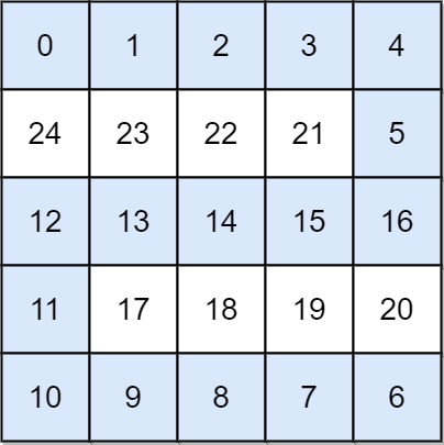
Input: grid = [[0,1,2,3,4],[24,23,22,21,5],[12,13,14,15,16],[11,17,18,19,20],[10,9,8,7,6]] Output: 16 Explanation: The final route is shown. We need to wait until time 16 so that (0, 0) and (4, 4) are connected.
Constraints:
n =grid.length=n =grid[i].length=1 <n <= 50=0 <grid[i][j] < n=2- Each value
grid[i][j]is unique.
※ 2.16.5.1. Constraints and Edge Cases
- Edge cases tested:
- Nonzero grid.
- Winding or blocked paths.
- Arbitrarily high or low elevational arrangements.
※ 2.16.5.2. My Solution (Code)
※ 2.16.5.2.1. v0 wrong, has logical bugs
1: from collections import defaultdict, deque 2: 3: class Solution: 4: │ def swimInWater(self, grid: List[List[int]]) -> int: 5: │ │ DIRS = [(-1, 0), (1, 0), (0, 1), (0,-1)] 6: │ │ ROWS, COLS = len(grid), len(grid[0]) 7: │ │ # i want to map the height to the locations: 8: │ │ height_to_cells = defaultdict(set) 9: │ │ visited = [[False] * COLS for r in range(ROWS)] 10: │ │ for r in range(ROWS): 11: │ │ │ for c in range(COLS): 12: │ │ │ │ height_to_cells[grid[r][c]].add((r, c)) 13: │ │ │ │ 14: │ │ # do I need a union find? -- I can just do a visited check 15: │ │ 16: │ │ # now we start the bfs: 17: │ │ q = deque([(0, 0)]) 18: │ │ visited[0][0] = True 19: │ │ level = 0 20: │ │ while q: 21: │ │ │ new_candidates = [] 22: │ │ │ for _ in range(len(q)): 23: │ │ │ │ r, c = q.popleft() 24: │ │ │ │ valid_neis = ((r + dr, c + dc) for dr, dc in DIRS if 0 <= r + dr < ROWS and 0 <= c + dc < COLS and grid[r+dr][c + dc] <= level + 1 and not visited[r + dr][c + dc]) 25: │ │ │ │ 26: │ │ │ │ for nei in valid_neis: 27: │ │ │ │ │ new_candidates.append(nei) 28: │ │ │ │ │ 29: │ │ │ │ valid_levels = ((l, height_to_cells[l]) for l in range(level + 1) if l in height_to_cells) 30: │ │ │ │ for cell_level, cells in valid_levels: 31: │ │ │ │ │ if len(cells) == 0: 32: │ │ │ │ │ │ del height_to_cells[cell_level] 33: │ │ │ │ │ re_introduced_cells = [ 34: │ │ │ │ │ │ (c_row, c_col) 35: │ │ │ │ │ │ for c_row, c_col in cells 36: │ │ │ │ │ │ if (not visited[c_row][c_col]) and 37: │ │ │ │ │ │ any( 38: │ │ │ │ │ │ │ visited[dr + c_row][dc + c_col] 39: │ │ │ │ │ │ │ for dr, dc in DIRS 40: │ │ │ │ │ │ │ if 0 <= dr + c_row < ROWS and 0 <= dc + c_col < COLS 41: │ │ │ │ │ │ ) 42: │ │ │ │ │ ] 43: │ │ │ │ │ 44: │ │ │ │ │ new_candidates.extend(re_introduced_cells) 45: │ │ │ for row, col in new_candidates: 46: │ │ │ │ visited[row][col] = True 47: │ │ │ │ if row == ROWS - 1 and col == COLS - 1: 48: │ │ │ │ │ return level + 1 49: │ │ │ │ │ 50: │ │ │ q.extend(new_candidates) 51: │ │ │ level += 1 52: │ │ │ 53: │ │ return level
technically this is a bruteforce attempt and what it’s trying to do is it’s doing a grid scan each time to try and get the next candidates.
this is why it’s extremely slow.
※ 2.16.5.2.2. v1 correct, guided Flood-fill, Dijsktra-like approach
1: from collections import defaultdict, deque 2: import heapq 3: 4: class Solution: 5: │ def swimInWater(self, grid: List[List[int]]) -> int: 6: │ │ # start from S, end at D, fastest hops possible 7: │ │ # prioritise the smallest elevation so far 8: │ │ ROWS, COLS = len(grid), len(grid[0]) 9: │ │ DIRS = [(0, 1), (0, -1), (1, 0), (-1, 0)] 10: │ │ visited = [[False] * COLS for _ in range(ROWS)] 11: │ │ 12: │ │ # GOTCHA: we can't assume that the first will be elevation = 0, so we have to read it from the grid. 13: │ │ heap = [(grid[0][0], (0,0))] 14: │ │ visited[0][0] = True 15: │ │ while heap: 16: │ │ │ t, (r, c) = heapq.heappop(heap) 17: │ │ │ # first reach of the target 18: │ │ │ if r == ROWS - 1 and c == COLS - 1: 19: │ │ │ │ return t 20: │ │ │ │ 21: │ │ │ for row, col in ((r + dr, c + dc) for dr, dc in DIRS 22: │ │ │ │ │ │ │ │ if 0 <= r + dr < ROWS and 0 <= c + dc < COLS 23: │ │ │ │ │ │ │ │ │and not visited[r + dr][c + dc] 24: │ │ │ │ │ │ │ │ ): 25: │ │ │ │ # visit it: 26: │ │ │ │ visited[row][col] = True 27: │ │ │ │ # NOTE: if we're accessing this later in time (e.g. cuz it was an island or something) then we need to respect the current time that's why we need to max this like so: 28: │ │ │ │ new_time = max(t, grid[row][col]) 29: │ │ │ │ heapq.heappush(heap, (new_time,(row, col)))
- Complexity Analysis
- Time Complexity:
- The grid is \(n * n\).
- Each cell can enter the heap only once, so \(O(n^2)\) heap operations.
- Each heap operation (push/pop) is \(O(log(n^{2})) = O(logn)\).
- Each cell checks up to four neighbors.
- Total: \(O(n^{2}\logn)\)
- The grid is \(n * n\).
- Space Complexity:
- Visited array: \(O(n^2)\)
- Heap: up to \(O(n^{2})\) elements in worst-case.
- Time Complexity:
- Explanation:
- You use a priority queue (min-heap) to always expand the cell with the smallest current elevation requirement.
- Each move records the maximum of the time to that cell and its elevation (since you can’t reach a cell until the water is at least that high).
- You only mark a cell as visited the first time it is placed into the heap; this is fine because the elevation (and thus cost to reach the cell) cannot be improved at a later time due to unique heights and the monotonic flood from 0 upwards.
※ 2.16.5.2.3. v2 Binary Search Approach
1: from collections import deque 2: 3: class Solution: 4: │ def swimInWater(self, grid): 5: │ │ n = len(grid) 6: │ │ 7: │ │ def can_reach(t): 8: │ │ │ """ 9: │ │ │ Helper function to check if it's possible to swim from (0,0) to (n-1,n-1) 10: │ │ │ if water level is 't' (i.e., you can only enter cells where elevation <= t). 11: │ │ │ Uses BFS for reachability. 12: │ │ │ """ 13: │ │ │ # If the starting cell is higher than t, cannot start swimming yet 14: │ │ │ if grid[0][0] > t: 15: │ │ │ │ return False 16: │ │ │ │ 17: │ │ │ visited = [[False]*n for _ in range(n)] 18: │ │ │ queue = deque([(0, 0)]) 19: │ │ │ visited[0][0] = True 20: │ │ │ 21: │ │ │ # BFS to explore reachable cells under water level t 22: │ │ │ while queue: 23: │ │ │ │ r, c = queue.popleft() 24: │ │ │ │ 25: │ │ │ │ # Check if we've reached the target cell 26: │ │ │ │ if r == n - 1 and c == n - 1: 27: │ │ │ │ │ return True 28: │ │ │ │ │ 29: │ │ │ │ # Explore 4-directional neighbors 30: │ │ │ │ for dr, dc in [(-1, 0), (1, 0), (0, -1), (0, 1)]: 31: │ │ │ │ │ nr, nc = r + dr, c + dc 32: │ │ │ │ │ # Check boundaries and if we can move into the neighbor cell 33: │ │ │ │ │ if (0 <= nr < n and 0 <= nc < n and 34: │ │ │ │ │ │ not visited[nr][nc] and 35: │ │ │ │ │ │ grid[nr][nc] <= t): 36: │ │ │ │ │ │ visited[nr][nc] = True 37: │ │ │ │ │ │ queue.append((nr, nc)) 38: │ │ │ │ │ │ 39: │ │ │ # If BFS finishes without reaching end, return False 40: │ │ │ return False 41: │ │ │ 42: │ │ # The minimum time to wait is at least the max of start and end elevations 43: │ │ left, right = max(grid[0][0], grid[-1][-1]), n * n - 1 44: │ │ 45: │ │ # Binary search for the minimum water level t that allows swimming through 46: │ │ while left < right: 47: │ │ │ mid = (left + right) // 2 48: │ │ │ if can_reach(mid): 49: │ │ │ │ # If reachable, try lower water levels 50: │ │ │ │ right = mid 51: │ │ │ else: 52: │ │ │ │ # If not, increase water level 53: │ │ │ │ left = mid + 1 54: │ │ │ │ 55: │ │ return left
Actually the binary search is slower than expected against the population, though memory efficient.
None
- Intuition: the elevation is a monotonically increasing range that we can test
- You ask: “Is it possible to swim to (n-1, n-1) if water is at level t?” If so, try lower; if not, try higher.
- Since elevations are unique and range from \(0\) to \(n^{2} - 1\), you could binary search the time \(t\) and for each, check (via BFS or DFS) whether you can reach \((n-1, n-1)\) if blocked by grid values > t.
- Binary search: \(O(\logn^{2})\) iterations, each doing \(O(n^{2})\) traversal ⇒ \(O(n^{2}\logn)\)
※ 2.16.5.2.4. v3 correct Kruskal’s Approach
1: class UnionFind: 2: │ def __init__(self, n): 3: │ │ # Initialize parent list where each node is its own parent (representative) 4: │ │ self.parent = list(range(n)) 5: │ │ 6: │ def find(self, x): 7: │ │ # Find the root parent (representative) of x with path compression 8: │ │ # Path compression flattens the tree by making each node point directly to the root 9: │ │ if x != self.parent[x]: 10: │ │ │ self.parent[x] = self.find(self.parent[x]) 11: │ │ return self.parent[x] 12: │ │ 13: │ def union(self, x, y): 14: │ │ # Union the sets containing x and y 15: │ │ # Returns False if x and y already belong to the same set 16: │ │ px, py = self.find(x), self.find(y) 17: │ │ if px == py: 18: │ │ │ return False # already connected 19: │ │ self.parent[px] = py # attach one tree under the other 20: │ │ return True 21: │ │ 22: class Solution: 23: │ def swimInWater(self, grid): 24: │ │ n = len(grid) 25: │ │ 26: │ │ if n == 1: # handle the trivial return case 27: │ │ │ return 0 28: │ │ │ 29: │ │ # Helper to convert 2D grid coordinates (r, c) into 1D index for Union-Find 30: │ │ def idx(r, c): 31: │ │ │ return r * n + c 32: │ │ │ 33: │ │ edges = [] # list of edges in the graph as (weight, node1, node2) 34: │ │ 35: │ │ # Generate edges between all pairs of adjacent cells (right and down neighbors) 36: │ │ # Weight of edge = max elevation of the two nodes (cells) 37: │ │ for r in range(n): 38: │ │ │ for c in range(n): 39: │ │ │ │ if r + 1 < n: 40: │ │ │ │ │ weight = max(grid[r][c], grid[r+1][c]) 41: │ │ │ │ │ edges.append((weight, idx(r, c), idx(r+1, c))) 42: │ │ │ │ if c + 1 < n: 43: │ │ │ │ │ weight = max(grid[r][c], grid[r][c+1]) 44: │ │ │ │ │ edges.append((weight, idx(r, c), idx(r, c+1))) 45: │ │ │ │ │ 46: │ │ # Sort all edges by ascending weight (height) 47: │ │ edges.sort() 48: │ │ 49: │ │ uf = UnionFind(n * n) # initialize union-find for all nodes 50: │ │ 51: │ │ # Process edges in order of increasing weight 52: │ │ for height, u, v in edges: 53: │ │ │ uf.union(u, v) # connect the two nodes in the union-find structure 54: │ │ │ 55: │ │ │ # After each union, check if start (top-left cell) and end (bottom-right) are connected 56: │ │ │ if uf.find(0) == uf.find(n * n - 1): 57: │ │ │ │ # The earliest time when the start and end belong to the same connected component 58: │ │ │ │ # is the required minimal water level 59: │ │ │ │ return height
※ 2.16.5.3. My Approach/Explanation
so my v0 had some intuition for getting all possible, but it was convoluted so there ended up being a bunch of bugs there
the key idea is that we have a new way of doing the candidate-selection. We need a DS to help us choose it fast.
What we want to do is to clear out the lowest elevation cells first, so that shall be the factor to prioritise. We just use a PQ for this. This ends up being somewhat similar to Dijkstras.
※ 2.16.5.4. My Learnings/Questions
I think this is a somewhat manageable extension to the usual flood fill. My v1 approach is a recognized as a variation of Dijkstra’s algorithm, where the minimum “max-elevation” along the path is the metric we wish to minimize.
AA: Yes! This is exactly the key—think of “flood fill, but you want the least maximum cell elevation on any path.” This turns Dijkstra’s into a “min-max” path problem.
The priority in the heap is the maximal elevation so far along the path to a cell.
The path that reaches the end with the smallest such maximum is the answer.
TRICK: 2D \(\implies\) 1D index flattening
we can flatten 2D indices into 1D for grids by doing this :
idx = lambda r, c: r * n + c # flatten 2D to 1Dthis is wild.
- Alternatives :
- Binary Search Approach (see v2 above)
Kruskal’s Algo Order Intuition: Treat as “flooding”, tracking when start and end become part of the same flooded region.
Union-Find (Kruskal’s Algorithm Order)
You can process all cells sorted by elevation, connecting adjacent open cells as the water “rises”, and use Union-Find to check when start and end become connected.
Complexity \(O(n^{2}\log(n^{2}))\) for sorting, then nearly linear with path compression.
- Careful in this question about :
- elevation of the start cell
- the max function on the time
※ 2.16.5.5. [Optional] Additional Context
I think this is a fair extension to the usual flood fill approaches.
Has a rich variety of ways to solve it, interesting!
※ 2.16.5.6. Retros
Honestly, I’ll just stick to the dijkstra’s approach here, it works and I know that it will work.
I know that it’s not optimal, but it works and I’ll be able to come up with it.
the binary search approach is intuitive as well.
※ 2.16.6. [123] ⭐️ Alien Dictionary (269) redo tedius hard Kahns_algo topological_sort
Given a list of words sorted lexicographically according to the rules of a new alien language, return a string representing the characters in the alien language sorted in their lexicographical order.
If there are multiple valid orders, return any of them.
If it is impossible to determine a valid order that satisfies all the words (i.e., the ordering is contradictory), return an empty string.
You can assume:
- All letters are lowercase English letters.
- The dictionary given is sorted according to the alien language rules.
- The order of letters is a total order on the letters that appear in the input.
Examples:
Input: words = [“wrt”,“wrf”,“er”,“ett”,“rftt”] Output: “wertf”
Explanation: From “wrt” and “wrf”, we get ’t’ < ’f’. From “wrt” and “er”, we get ’w’ < ’e’. And so on, combining all inferred orders gives one valid character order.
—
LeetCode: Alien Dictionary (Problem)
There is a new alien language, but we don’t know the order of the letters.
You are given a list of words sorted lexicographically by the rules of this new language. Derive the order of letters in this language.
Return a string of unique letters in the new alien language sorted lexicographically according to the rules.
If there are multiple valid orders, return any of them.
If it is impossible to determine the order, return an empty string.
Constraints:
- 1 <= words.length <= 100
- 1 <= words[i].length <= 100
- words[i] consists of only lowercase English letters.
Example:
Input: words = [“wrt”,“wrf”,“er”,“ett”,“rftt”] Output: “wertf”
Explanation: From the given order of words, you can deduce the order of letters by comparing adjacent words and finding the first letter that differs. This produces a partial order of letters which you must combine into a total order.
—
Notes:
Both problems are essentially the same: they require you to infer a character order (topological ordering) from a sorted word list, detecting if the order is possible or contradictory.
If you want, I can help you write down a canonical problem statement combining these perspectives or give you a step-by-step outline for recording.
Let me know!
※ 2.16.6.1. Constraints and Edge Cases
Have some edge cases to consider like invalid ordering and such (referring to the rule 2)
Also possibly need to do cycle detection.
※ 2.16.6.2. My Solution (Code)
※ 2.16.6.2.1. v0: failed, some logical bugs from the radix approach:
1: from collections import deque, defaultdict 2: 3: class Solution: 4: │ def foreignDictionary(self, words: List[str]) -> str: 5: │ │ # char to other chars: 6: │ │ graph = defaultdict(list) 7: │ │ indegree = [0] * 26 8: │ │ 9: │ │ # now we form the graph: 10: │ │ place = 0 11: │ │ while place < 100: 12: │ │ │ chars = [word[place] for word in words if len(word) > place] 13: │ │ │ if not chars or len(chars) == 1: # can stop gathering edges 14: │ │ │ │ break 15: │ │ │ │ 16: │ │ │ for i in range(1, len(chars)): 17: │ │ │ │ u, v = chars[i - 1], chars[i] 18: │ │ │ │ graph[u].append(v) 19: │ │ │ │ indegree[ord(v) - ord('a')] += 1 20: │ │ │ │ 21: │ │ │ place += 1 22: │ │ │ 23: │ │ topo = [] 24: │ │ graph_keys = list(graph.keys()) 25: │ │ # sorted by the graph insertion order 26: │ │ no_deps_candidates = sorted([u_idx for u_idx in range(26) if indegree[u_idx] == 0], key=lambda x:graph_keys.index(chr(ord('a') + x))) 27: │ │ q = deque(no_deps_candidates) 28: │ │ 29: │ │ while q: 30: │ │ │ u_idx = q.popleft() 31: │ │ │ char = chr(ord('a') + u_idx) 32: │ │ │ topo.append(char) 33: │ │ │ 34: │ │ │ for nei in graph[char]: 35: │ │ │ │ nei_idx = ord(nei) - ord('a') 36: │ │ │ │ indegree[nei_idx] -= 1 37: │ │ │ │ if indegree[nei_idx] == 0: 38: │ │ │ │ │ q.append(nei_idx) 39: │ │ │ │ │ 40: │ │ return "".join(topo) 41:
- Your approach tries to:
- Iterate column by column (character-position by character-position in the words),
- Collect all characters at the current position in the sorted words,
- For consecutive different characters at this position, infer directed edges (from the earlier to the later character),
- Build a graph and an indegree array,
- Perform a topological sort by BFS (Kahn’s algorithm).
- Logical Bugs:
- Incorrect ordering of edges:
- You form edges between all consecutive characters at the same index position from the list of chars extracted only at that position.
- But simply looking at that column of characters without comparing adjacent words is not the correct approach.
- The ordering relation should be inferred only from pairs of adjacent words, specifically:
- For each pair of adjacent words (e.g. words[i] and words[i+1]), find the first index where they differ, and then infer the letter order from that differing character.
- Prefix ordering special case not handled:
- E.g., if a word is prefix of another, e.g., “abc” and “ab”, the order is invalid because shorter word should appear first for correct lex order.
- Indegree bookkeeping mistake:
- You use a list 26 for indegree, but your graph stores characters (str), not indices, *which can cause issues if some characters never appear as starting nodes.. This is precisely the main problem this solution faced.
- Vertices initialisation:
- You only create graph edges for characters that appear in those differing positions, but the alien alphabet consists of all unique characters in the input words.
- If some characters never appear as keys in your graph, they will be ignored in topo sort. This is the main flaw in my working.
- Ordering of zero indegree nodes enqueueing and output order may be inconsistent —
- sorting based on graph insertion order uses
graph_keys.index(...)which can cause issues when the character doesn’t exist or ordering is incomplete.
- sorting based on graph insertion order uses
- Incorrect ordering of edges:
Even if this is wrong, here’s an analysis of its complexity:
Time complexity:
Extracting pairs and building edges (if done properly) is \(O(N * L)\) where \(N\) is number of words and \(L\) is max word length, since you compare adjacent words.
Topological sort using BFS or DFS on up to 26 nodes (characters) is negligible \(O(V+E)\), as only lowercase letters.
Your code does more work by collecting chars column-wise, but a proper implementation focuses on adjacent word pairs.
Space complexity:
The graph stores up to 26 nodes and edges up to \(O(26^2)\) in worst case.
Indegree array fixed size 26.
- Extract edges only by comparing adjacent words and finding first differing character.
- Initialize your graph nodes with all unique characters found in the words.
- Implement Kahn’s algorithm cleanly with meaningful variable names.
- Handle prefix invalid cases: if
word1is longer andword2is prefix ofword1, return""as invalid. - Use Python sets and dictionaries to represent the graph nodes and edges.
- For clarity, build a helper function to compare pairs of words.
※ 2.16.6.2.2. v1: canonical optimal, pairwise comparison
1: from collections import defaultdict, deque 2: from typing import List 3: 4: class Solution: 5: │ def alienOrder(self, words: List[str]) -> str: 6: │ │ # Step 1: Initialize data structures 7: │ │ # Graph: character -> set of characters it precedes (adjacency list) 8: │ │ graph = defaultdict(set) 9: │ │ # Indegree count of each node (character) 10: │ │ indegree = {c:0 for word in words for c in word} 11: │ │ 12: │ │ # Step 2: Build graph edges from adjacent pairs 13: │ │ for i in range(len(words) - 1): 14: │ │ │ w1, w2 = words[i], words[i+1] 15: │ │ │ 16: │ │ │ # Check for prefix case where w1 is longer but w2 is prefix -> invalid 17: │ │ │ if len(w1) > len(w2) and w1.startswith(w2): 18: │ │ │ │ return "" 19: │ │ │ │ 20: │ │ │ # Find first differing character 21: │ │ │ for c1, c2 in zip(w1, w2): 22: │ │ │ │ if c1 != c2: 23: │ │ │ │ │ # Add edge c1 -> c2 if not already added 24: │ │ │ │ │ if c2 not in graph[c1]: 25: │ │ │ │ │ │ graph[c1].add(c2) 26: │ │ │ │ │ │ indegree[c2] += 1 27: │ │ │ │ │ break # Only first differing character per pair is relevant 28: │ │ │ │ │ 29: │ │ # Step 3: Topological sort (Kahn's Algorithm) 30: │ │ # Start with nodes that have zero indegree 31: │ │ queue = deque([c for c in indegree if indegree[c] == 0]) 32: │ │ output = [] 33: │ │ 34: │ │ while queue: 35: │ │ │ c = queue.popleft() 36: │ │ │ output.append(c) 37: │ │ │ for nei in graph[c]: 38: │ │ │ │ indegree[nei] -= 1 39: │ │ │ │ if indegree[nei] == 0: 40: │ │ │ │ │ queue.append(nei) 41: │ │ │ │ │ 42: │ │ # Step 4: If output length differs from unique chars count, cycle detected 43: │ │ if len(output) != len(indegree): 44: │ │ │ return "" 45: │ │ │ 46: │ │ return "".join(output)
The canonical solution is:
- Identify all unique characters as graph nodes.
- For each pair of adjacent words, find the first differing character and create a directed edge from the character in
word1to that inword2. - Detect invalid cases (prefix conflicts).
- Perform a topological sort to derive character ordering.
- If cycle detected or impossible ordering, return
"".
This approach is optimal and uses simple data structures suitable for constraints.
※ 2.16.6.3. My Approach/Explanation
my v0 idea was to attempt to do a topo sort.
What I did notice was that this problem felt like it had elements of:
- some kind of topo sorting
- some kind of caring about prefix-matching
- some kind of radix approach where we should compare places of characters.
Turns out there are some logical bugs in it.
※ 2.16.6.4. My Learnings/Questions
Why pairwise adjacent words?
Because lexical order is built from comparing consecutive words; non-adjacent word comparisons do not add valid constraints.
- I’m not sure how to get the right intuition from the get-go. I had the wrong intuition here that it should be a radix approach where I try to build a graph then get a topo ordering out of it.
※ 2.16.6.5. [Optional] Additional Context
I think the intuition is right here, but the implementation’s flaws (focusing on a radix-approach instead of the pairwise comparisons).
AA: Your initial approach has logical bugs mainly in how you built edges (from a column-wise scan rather than adjacent word pairs) and in incomplete handling of edge cases
※ 2.16.6.6. Retros
I think this is just a tedius example.
It’s possible to break this down into multiple steps incrementally after we get the intuition that we’re just building a topo sort.
Show/Hide Python Code1: from collections import defaultdict, deque 2: from typing import List 3: 4: class Solution: 5: │ def foreignDictionary(self, words: List[str]) -> str: 6: │ │ # node is a character, to its neighbours 7: │ │ adj = defaultdict(set) 8: │ │ # maps char to indegree: 9: │ │ indegree = {char:0 for word in words for char in word} 10: │ │ n = len(words) 11: │ │ 12: │ │ # edges ?? ==> create the edges now n nodes have n - 1 edges 13: │ │ # we use adjacent pairs to build graph edges: 14: │ │ for idx in range(n - 1): 15: │ │ │ # pairwise judgement: 16: │ │ │ w1, w2 = words[idx], words[idx + 1] 17: │ │ │ 18: │ │ │ # prefix case [invalid case]: when w1 is longer but w2 is prefix: 19: │ │ │ if (len(w1) > len(w2)) and w1.startswith(w2): 20: │ │ │ │ # note: this prefix case that is invalid is from the second condition that they've stated 21: │ │ │ │ return "" 22: │ │ │ │ 23: │ │ │ # we find first differring char in them: 24: │ │ │ for c1, c2 in zip(w1, w2): 25: │ │ │ │ if c1 != c2: 26: │ │ │ │ │ # then we add edge c1 -> c2 if it's not already added: 27: │ │ │ │ │ # c1 is lower in lexical order because the input is in "lexical" order 28: │ │ │ │ │ if c2 not in adj[c1]: 29: │ │ │ │ │ │ adj[c1].add(c2) 30: │ │ │ │ │ │ indegree[c2] += 1 31: │ │ │ │ │ break 32: │ │ │ │ │ 33: │ │ # now we can topo sort as per usual: 34: │ │ queue = deque([c for c in indegree if indegree[c] == 0]) 35: │ │ topo_sorted = [] 36: │ │ 37: │ │ while queue: 38: │ │ │ c = queue.popleft() 39: │ │ │ topo_sorted.append(c) 40: │ │ │ for nei in adj[c]: 41: │ │ │ │ indegree[nei] -= 1 42: │ │ │ │ if indegree[nei] == 0: 43: │ │ │ │ │ queue.append(nei) 44: │ │ │ │ │ 45: │ │ # cycle detection! 46: │ │ if len(topo_sorted) != len(indegree): 47: │ │ │ return "" 48: │ │ │ 49: │ │ return "".join(topo_sorted)
※ 2.16.7. [124] Cheapest Flights Within K Stops (787) bellman_ford almost confounding_gotcha
There are n cities connected by some number of flights. You are given
an array flights where
flights[i] = [from=_{=i}=, to=i=, price=i=]= indicates that
there is a flight from city from=_{=i} to city to=_{=i} with cost
price=_{=i}.
You are also given three integers src, dst, and k, return the
cheapest price from src to dst with at most k stops. If
there is no such route, return // -1.
Example 1:
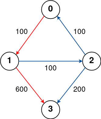
Input: n = 4, flights = [[0,1,100],[1,2,100],[2,0,100],[1,3,600],[2,3,200]], src = 0, dst = 3, k = 1 Output: 700 Explanation: The graph is shown above. The optimal path with at most 1 stop from city 0 to 3 is marked in red and has cost 100 + 600 = 700. Note that the path through cities [0,1,2,3] is cheaper but is invalid because it uses 2 stops.
Example 2:
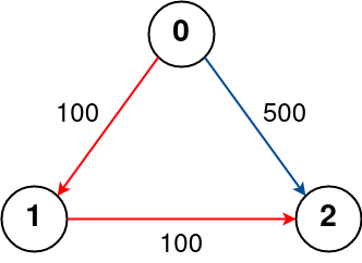
Input: n = 3, flights = [[0,1,100],[1,2,100],[0,2,500]], src = 0, dst = 2, k = 1 Output: 200 Explanation: The graph is shown above. The optimal path with at most 1 stop from city 0 to 2 is marked in red and has cost 100 + 100 = 200.
Example 3:
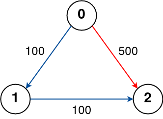
Input: n = 3, flights = [[0,1,100],[1,2,100],[0,2,500]], src = 0, dst = 2, k = 0 Output: 500 Explanation: The graph is shown above. The optimal path with no stops from city 0 to 2 is marked in red and has cost 500.
Constraints:
1 <n <= 100=0 <flights.length <= (n * (n - 1) / 2)=flights[i].length =3=0 <from=i=, to=i= < n=from=_{=i}= != to=i1 <price=i= <= 10=4- There will not be any multiple flights between two cities.
0 <src, dst, k < n=src !dst=
※ 2.16.7.1. Constraints and Edge Cases
- No path exists: returns -1 correctly.
k = 0(no stops allowed): finds only direct connections.- Multiple flights, cycles: both approaches avoid cycles or infinite revisiting.
※ 2.16.7.2. My Solution (Code)
※ 2.16.7.2.1. v0: wrong, correct structure and intuition
this one is just an execution not accurate enough issue.
1: class Solution: 2: │ def findCheapestPrice(self, n: int, flights: List[List[int]], src: int, dst: int, k: int) -> int: 3: │ │ # single src to single dest 4: │ │ dist = [float('inf')] * n 5: │ │ dist[src] = 0 6: │ │ 7: │ │ # we relax the edges for k times: 8: │ │ for _ in range(k): 9: │ │ │ tmp = dist.copy() 10: │ │ │ for u, v, w in flights: 11: │ │ │ │ can_relax = dist[u] != float('inf') and dist[u] + w < tmp[v] 12: │ │ │ │ if can_relax: 13: │ │ │ │ │ tmp[v] = dist[u] + w 14: │ │ │ dist = tmp 15: │ │ │ 16: │ │ if dist[dst] == float('inf'): 17: │ │ │ return -1 18: │ │ │ 19: │ │ return dist[dst]
Improvements:
Relaxation Count (\(k+1\) Times, Not \(k\))
You should relax the edges \(k+1\) times (not \(k\) times), because paths with up to \(k\) stops can contain up to \(k+1\) edges. If you relax for only k iterations, you might miss some paths.
⭐️ Edge Relaxation Must Use a Copy (to Prevent “Greedy” Updating)
In each iteration, you must use the distances from the previous iteration during relaxations, rather than updating dist in place, because otherwise, in the same iteration, you might use a newly updated value of dist from a parallel path, which allows for more than k stops in effect. This is a very common pitfall!
Fix: Use a \(temp = dist.copy()\) for each iteration and only update temp, then at the end, assign
dist = temp.
※ 2.16.7.2.2. v1: bellman ford k + 1 iterations, uses temp store to avoid parallel executions confounding each other
class Solution: │ def findCheapestPrice(self, n: int, flights: List[List[int]], src: int, dst: int, k: int) -> int: │ │ # single src to single dest │ │ dist = [float('inf')] * n │ │ dist[src] = 0 │ │ │ │ # we relax the edges for k times: │ │ for _ in range(k + 1): │ │ │ tmp = dist.copy() │ │ │ for u, v, w in flights: │ │ │ │ can_relax = dist[u] != float('inf') and dist[u] + w < tmp[v] │ │ │ │ if can_relax: │ │ │ │ │ tmp[v] = dist[u] + w │ │ │ dist = tmp │ │ │ │ │ if dist[dst] == float('inf'): │ │ │ return -1 │ │ │ │ │ return dist[dst]
- Complexity Analysis
- Time: For each of k+1 rounds, iterate through all edges:
- \(O(k * E)\) where \(E\) = number of flights
- Worst case \(E\approx n^2\), so upper bound is \(O(n^3)\), but for max \(n=100\), this is fine in practice.
- Space:
- Distance array: \(O(n)\)
- Temporary copy: \(O(n)\)
- Time: For each of k+1 rounds, iterate through all edges:
※ 2.16.7.2.3. v2: alternative: early returns from typical BFS: Shortest path in up-to-k steps
1: from collections import defaultdict, deque 2: class Solution: 3: │ def findCheapestPrice(self, n: int, flights: List[List[int]], src: int, dst: int, k: int) -> int: 4: │ │ graph = defaultdict(list) 5: │ │ 6: │ │ # Build the adjacency list: u -> (v, cost) 7: │ │ for u, v, cost in flights: 8: │ │ │ graph[u].append((v, cost)) 9: │ │ │ 10: │ │ # Distance array to keep the minimum cost to reach each node 11: │ │ dist = [float('inf')] * n 12: │ │ dist[src] = 0 13: │ │ 14: │ │ # Queue: (stops, current node, current cost) 15: │ │ q = deque() 16: │ │ q.append((0, src, 0)) 17: │ │ 18: │ │ while q: 19: │ │ │ stops, node, curr_cost = q.popleft() 20: │ │ │ 21: │ │ │ # If the number of stops exceeds the limit, skip further processing 22: │ │ │ if stops > k: 23: │ │ │ │ continue 24: │ │ │ │ 25: │ │ │ for neighbor, price in graph[node]: 26: │ │ │ │ new_cost = curr_cost + price 27: │ │ │ │ if new_cost < dist[neighbor]: 28: │ │ │ │ │ dist[neighbor] = new_cost 29: │ │ │ │ │ q.append((stops + 1, neighbor, new_cost)) 30: │ │ │ │ │ 31: │ │ return -1 if dist[dst] == float('inf') else dist[dst]
This is also correct: it tracks number of stops taken along with cost.
It does early pruning: it only explores a path again if it found a better (cheaper) route to a node; however, it’s important to note that for some graphs, it’s possible to reach a node with more stops and a higher price, but a cheaper route to the destination in total. Since the problem wants the minimum path cost (not minimum steps), but with the constraint on stops, this heuristic can be accepted.
In practice, this BFS version also works (and is accepted), but Bellman-Ford is usually preferred for its clarity regarding the constraint.
Complexity Analysis:
Time:
Each node can be queued multiple times, but with \(k\) stops as the bound, in practice, it’s \(O(n * k)\) but can be higher if the graph is very dense.
Space:
Queue can store \(O(n * k)\) items in the worst case.
※ 2.16.7.3. My Approach/Explanation
This seems like a bellman ford type question with a limited number of hops. So if we take k hops, we have 2 cases :
- we don’t have an answer for the cell yet (between S and D) \(\implies\) not possible
- we have an answer
※ 2.16.7.4. My Learnings/Questions
- The bfs approach works but the bellman ford is a clearer implementation.
GOTCHA/TRICK: Snapshotting Trick
we can use a temp distances aux store to avoid confounding things within a run of bellman ford
In each iteration, you must use the distances from the previous iteration during relaxations, rather than updating dist in place, because otherwise, in the same iteration, you might use a newly updated value of dist from a parallel path, which allows for more than k stops in effect. This is a very common pitfall!
Fix: Use a \(temp = dist.copy()\) for each iteration and only update temp, then at the end, assign
dist = temp.- careful:
Remember that in bellman ford, we are relaxing edges on each iteration.
the objective here is to have correct estimates of path lengths with up to \(k\) stops, this means \(k\) vertices.
\(k\) vertices will have \(k + 1\) edges.
After the \(n^{th}\) iteration of bellman ford relaxation, the number of edges that are accurately estimated is \(n\).
※ 2.16.7.5. [Optional] Additional Context
Very close! Just have to be aware of the tricks and the gotchas.
※ 2.16.7.6. Retros
- Alright I couldn’t get the highest performing version of the code, but got the bellman-ford version of it though.
※ 2.16.8. [Depth-Blind] Sort Items by Groups Respecting Dependencies (1203) failed 2_phase_topological_sort topological_sorting
There are n items each belonging to zero or one of m groups where
group[i] is the group that the i-th item belongs to and it’s equal
to -1 if the i-th item belongs to no group. The items and the groups
are zero indexed. A group can have no item belonging to it.
Return a sorted list of the items such that:
- The items that belong to the same group are next to each other in the sorted list.
- There are some relations between these items where
beforeItems[i]is a list containing all the items that should come before thei-th item in the sorted array (to the left of thei-th item).
Return any solution if there is more than one solution and return an empty list if there is no solution.
Example 1:
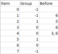
Input: n = 8, m = 2, group = [-1,-1,1,0,0,1,0,-1], beforeItems = [[],[6],[5],[6],[3,6],[],[],[]] Output: [6,3,4,1,5,2,0,7]
Example 2:
Input: n = 8, m = 2, group = [-1,-1,1,0,0,1,0,-1], beforeItems = [[],[6],[5],[6],[3],[],[4],[]] Output: [] Explanation: This is the same as example 1 except that 4 needs to be before 6 in the sorted list.
Constraints:
1 <m <= n <= 3 * 10=4group.length =beforeItems.length= n-1 <group[i] <= m - 1=0 <beforeItems[i].length <= n - 1=0 <beforeItems[i][j] <= n - 1=i !beforeItems[i][j]=- =beforeItems[i] =does not contain duplicates elements.
※ 2.16.8.1. Constraints and Edge Cases
<list constraints, input limits, or tricky edge cases here>
※ 2.16.8.2. My Solution (Code)
※ 2.16.8.2.1. v0: failed, conceptually wrong
1: from collections import defaultdict, deque 2: 3: class Solution: 4: │ def sortItems(self, n: int, m: int, group: List[int], beforeItems: List[List[int]]) -> List[int]: 5: │ │ # TODO this might need tweaking to account for groups 6: │ │ adj = defaultdict(list) 7: │ │ 8: │ │ # we build adj list together with the indegrees from beforeItems: 9: │ │ indegrees = [0] * (n) 10: │ │ for dest, sources in enumerate(beforeItems): 11: │ │ │ if not sources: 12: │ │ │ │ continue 13: │ │ │ │ 14: │ │ │ indegrees[dest] = len(sources) 15: │ │ │ for source in sources: 16: │ │ │ │ adj[source].append((dest, group[dest])) 17: │ │ │ │ 18: │ │ queue = deque(item for item, indegree in enumerate(indegrees) if indegree == 0) 19: │ │ 20: │ │ visited = 0 21: │ │ schedule = [] # we shall keep (item, group) within this 22: │ │ while queue: 23: │ │ │ item = queue.popleft() 24: │ │ │ visited += 1 25: │ │ │ 26: │ │ │ schedule.append(item) 27: │ │ │ for nei, nei_group in sorted(adj[item], key=lambda x: x[1]): 28: │ │ │ │ indegrees[nei] -= 1 29: │ │ │ │ # check if ready: 30: │ │ │ │ if indegrees[nei] == 0: 31: │ │ │ │ │ queue.append(nei) 32: │ │ │ │ │ 33: │ │ if not visited == n: 34: │ │ │ return [] 35: │ │ │ 36: │ │ return schedule
- this is actually similar to how SQL group by would do things: one index by another and topo sorting.
- in this case, we need to know that the order in which the groups appear matter.
- the ungrouped items should be formed into as many 1-group elements as possible so that we don’t need to work with ridiculous contraints.
Why two-phase topological sort is required:
Because some item dependencies create group-level dependencies (item in group A → item in group B enforces group A before group B). Naively topo sorting by items only can result in group items not being adjacent.
※ 2.16.8.2.2. v1: 2-phase topo sorting
1: from collections import defaultdict, deque 2: from typing import List 3: 4: class Solution: 5: │ def sortItems(self, n: int, m: int, group: List[int], beforeItems: List[List[int]]) -> List[int]: 6: │ │ # Step 0: Assign unique group IDs to ungrouped items, keep them in unique groups 7: │ │ new_gid = m 8: │ │ for i in range(n): 9: │ │ │ if group[i] == -1: 10: │ │ │ │ group[i] = new_gid 11: │ │ │ │ new_gid += 1 12: │ │ │ │ 13: │ │ # Step 1: Prepare adjacency lists + indegrees 14: │ │ group_adj, group_indeg = defaultdict(list), defaultdict(int) 15: │ │ item_adj, item_indeg = defaultdict(list), defaultdict(int) 16: │ │ 17: │ │ # Step 2: Build both graphs 18: │ │ for item in range(n): 19: │ │ │ for prev_item in beforeItems[item]: 20: │ │ │ │ # Build item dependency graph 21: │ │ │ │ item_adj[prev_item].append(item) 22: │ │ │ │ item_indeg[item] += 1 23: │ │ │ │ 24: │ │ │ │ # Build group dependency graph, only if they belong to different groups 25: │ │ │ │ if group[prev_item] != group[item]: 26: │ │ │ │ │ src, dest = group[prev_item], group[item] 27: │ │ │ │ │ group_adj[src].append(dest) 28: │ │ │ │ │ group_indeg[dest] += 1 29: │ │ │ │ │ 30: │ │ # Step 3: Topological sort helper 31: │ │ def topo(nodes, adj, indeg): 32: │ │ │ q = deque(x for x in nodes if indeg[x] == 0) 33: │ │ │ res = [] 34: │ │ │ while q: 35: │ │ │ │ u = q.popleft() 36: │ │ │ │ res.append(u) 37: │ │ │ │ for nei in adj[u]: 38: │ │ │ │ │ indeg[nei] -= 1 39: │ │ │ │ │ if indeg[nei] == 0: 40: │ │ │ │ │ │ q.append(nei) 41: │ │ │ return res if len(res) == len(nodes) else [] 42: │ │ │ 43: │ │ # Step 4: Get group order & item order 44: │ │ group_nodes = list(range(new_gid)) 45: │ │ group_order = topo(group_nodes, group_adj, group_indeg.copy()) 46: │ │ if not group_order: 47: │ │ │ return [] 48: │ │ │ 49: │ │ item_nodes = list(range(n)) 50: │ │ items_order = topo(item_nodes, item_adj, item_indeg.copy()) 51: │ │ if not items_order: 52: │ │ │ return [] 53: │ │ │ 54: │ │ # Step 5: Arrange items by group according to items_order 55: │ │ group_to_items = defaultdict(list) 56: │ │ for item in items_order: 57: │ │ │ group_to_items[group[item]].append(item) 58: │ │ │ 59: │ │ # Step 6: Build the final result 60: │ │ res = [] 61: │ │ for g in group_order: 62: │ │ │ res.extend(group_to_items[g]) 63: │ │ return res
※ 2.16.8.2.3. v2: single-graph approach
1: from collections import defaultdict, deque 2: from typing import List 3: 4: class Solution: 5: │ def sortItems(self, n: int, m: int, group: List[int], 6: │ │ │ │ │ beforeItems: List[List[int]]) -> List[int]: 7: │ │ """ 8: │ │ Single-graph approach for 1203. 9: │ │ Instead of 2 separate topo sorts (items, then groups), 10: │ │ we build one unified DAG containing: 11: │ │ │ - virtual group nodes 12: │ │ │ - item nodes 13: │ │ and run ONE topological sort on all of them. 14: │ │ """ 15: │ │ 16: │ │ # --- STEP 1: Assign unique group IDs to ungrouped items --- 17: │ │ # Problem states group[i] == -1 if no group. We give these items 18: │ │ # their own 'singleton' pseudo-group to enforce adjacency. 19: │ │ new_group_id = m 20: │ │ for i in range(n): 21: │ │ │ if group[i] == -1: 22: │ │ │ │ group[i] = new_group_id 23: │ │ │ │ new_group_id += 1 24: │ │ total_groups = new_group_id # updated count after assignment 25: │ │ 26: │ │ # --- STEP 2: Node indexing scheme --- 27: │ │ # 0..n-1 → item nodes 28: │ │ # n..n+total_groups-1 → virtual group nodes 29: │ │ def group_node(g_id: int) -> int: 30: │ │ │ """ Map a group ID to its virtual node index in the graph """ 31: │ │ │ return n + g_id 32: │ │ │ 33: │ │ # --- Data structures for graph + indegree --- 34: │ │ G = defaultdict(list) # adjacency list 35: │ │ indeg = defaultdict(int) # indegree dictionary 36: │ │ 37: │ │ # Initialize indegrees to zero for all nodes 38: │ │ all_nodes = list(range(n)) + [group_node(g) for g in range(total_groups)] 39: │ │ for node in all_nodes: 40: │ │ │ indeg[node] = 0 41: │ │ │ 42: │ │ # --- STEP 3: Connect each group node to the items it contains --- 43: │ │ # This ensures items of the same group appear *after* the group's 44: │ │ # node in topo order, making them contiguous in the final output. 45: │ │ for item in range(n): 46: │ │ │ gnode = group_node(group[item]) 47: │ │ │ G[gnode].append(item) 48: │ │ │ indeg[item] += 1 49: │ │ │ 50: │ │ # --- STEP 4: Add edges for dependencies --- 51: │ │ # For every beforeItems[i], item i must appear AFTER prev_item. 52: │ │ for item in range(n): 53: │ │ │ for prev_item in beforeItems[item]: 54: │ │ │ │ if group[item] == group[prev_item]: 55: │ │ │ │ │ # Same group → direct dependency between items 56: │ │ │ │ │ G[prev_item].append(item) 57: │ │ │ │ │ indeg[item] += 1 58: │ │ │ │ else: 59: │ │ │ │ │ # Different groups → dependency between group nodes 60: │ │ │ │ │ G[group_node(group[prev_item])].append(group_node(group[item])) 61: │ │ │ │ │ indeg[group_node(group[item])] += 1 62: │ │ │ │ │ 63: │ │ # --- STEP 5: Kahn's Algorithm (BFS Topological Sort) --- 64: │ │ q = deque([node for node in all_nodes if indeg[node] == 0]) 65: │ │ topo_order = [] 66: │ │ 67: │ │ while q: 68: │ │ │ u = q.popleft() 69: │ │ │ topo_order.append(u) 70: │ │ │ for v in G[u]: 71: │ │ │ │ indeg[v] -= 1 72: │ │ │ │ if indeg[v] == 0: 73: │ │ │ │ │ q.append(v) 74: │ │ │ │ │ 75: │ │ # --- STEP 6: Check for cycles --- 76: │ │ # A cycle anywhere (items or groups) means no valid order exists. 77: │ │ if len(topo_order) != len(all_nodes): 78: │ │ │ return [] 79: │ │ │ 80: │ │ # --- STEP 7: Extract only items from topo_order --- 81: │ │ # Group nodes were just helpers to enforce contiguous grouping. 82: │ │ result = [node for node in topo_order if node < n] 83: │ │ return result 84: │ │ 85:
※ 2.16.8.3. My Approach/Explanation
- I failed to realise that the topo sorting needed to be done in 2 dimensions. I think I need more sleep.
※ 2.16.8.4. My Learnings/Questions
- 2 phase topo sorting isn’t that hard.
※ 2.16.8.5. [Optional] Additional Context
I failed in this because of a comprehension issue.
※ 2.17. 2-D DP
| Headline | Time | ||
|---|---|---|---|
| Total time | 7:08 | ||
| 2-D DP | 7:08 | ||
| [125] Unique Paths (62) | 0:31 | ||
| [126] Longest Common Subsequence (1143) | 0:28 | ||
| [127] ⭐️ Best Time to Buy and Sell… | 0:31 | ||
| [128] Coin Change II (518) | 0:21 | ||
| [129] ⭐️ Target Sum (494) | 0:13 | ||
| [130] Interleaving String (97) | 1:23 | ||
| [131] Longest Increasing Path in a… | 0:46 | ||
| [132] Distinct Subsequences (115) | 0:52 | ||
| [133] Edit Distance (72) | 0:49 | ||
| [134] ⭐️ Burst Balloons (312) | 0:15 | ||
| [135] Regular Expression Matching (10) | 0:59 |
※ 2.17.1. General Notes
※ 2.17.1.1. Fundamentals
※ 2.17.1.2. Tricks
※ 2.17.1.3. TODO Canonical Problems for DP
※ 2.17.1.3.1. Knapsack Problems
| Variant | Unlimited Supply? | DP Update Pattern | Example Problem | |
|---|---|---|---|---|
| 1. 0/1 Knapsack | Only once | for each `num` in `nums`, for `t` from target to num: `dp[t] | = dp[t-num]` | Subset sum; Partition problem (416) |
| 2. Unbounded Knapsack | Infinite times | for each `num`, for `t` from num to target: `dp[t] | = dp[t-num]` | Coin change infinite supply |
| 3. Bounded Knapsack | Up to limited times | “Decompose” item frequency with binary trick or bounded DP | If each num is present with count | |
| 4. Classic Value Knapsack | With values and weights | Use dp table `dp[i][w] = max value` | Standard 0/1/Unbounded knapsack |
some examples:
※ 2.17.1.3.2. String / Sequence Problems
see this generic description of why subsequences are interesting.
Summary Table of Key Mental Models for Subsequences
| Property | Implication | Common Technique |
|---|---|---|
| Relative order preserved | Use scanning, two pointers, indices to maintain order | Two-pointer greedy check, DP |
| Exponential subsequences count | Explicit enumeration expensive — count with DP | Memoization, DP counting |
| Include/exclude characters | DP relation: total = include char + exclude char | Classic DP subset & subsequence recurrences |
| Handling duplicates | Deduplicate counting carefully | Track last occurrence indices |
| Non-contiguity | Allows flexible skipping | Allows binary choices, recursive branching |
| Different from substrings | Faster checks possible | Simplified DP vs substring matching |
Understanding subsequences properly is critical for solving classic and advanced string problems efficiently. Here are the unique properties and mental models that will help you quickly recognize and solve problems involving subsequences: *** ## What is Special About the Definition of Subsequences - A **subsequence** is formed by deleting zero or more characters from the original string **without changing the relative order** of the remaining characters. - Unlike substrings, subsequences do **not require contiguity**. - This means all substrings are subsequences, but the opposite is not true. - The flexibility of skipping characters while maintaining order is key to most subsequence problems. *** ## Unique Properties and Mental Models to Leverage 1. **Relative Order Preservation** │ - All elements chosen appear in the same order as the original string. │ - This suggests many algorithms can be designed via **two-pointer techniques**, dynamic programming, or backtracking to **match characters in sequence**. │ - For instance, checking if `T` is a subsequence of `S` involves iterating through `S` and trying to "cover" characters of `T` in order. │ 2. **Exponential Number of Subsequences** │ - For a string of length `n`, there are $$2^n$$ possible subsequences. │ - Enumerating all subsequences naïvely is expensive, so many algorithms use memoization or DP to **count** subsequences without generating them. │ 3. **Dynamic Programming Structure** │ - Subsequence problems usually exhibit **optimal substructure** and **overlapping subproblems**, which make them ideal for DP. │ - Common DP relations track prefixes of strings (e.g., `dp[i][j]` meaning # of subsequences of `s[:i]` matching `t[:j]`). │ 4. **Additive Nature of Subsequences** │ - Including or excluding a character independently leads to a recurrence where: │ │- The number of subsequences including the current character + number excluding it = total subsequences so far. │ - Helps in counting distinct subsequences and variants. │ 5. **Subsequence Matching Is Different from Substring Matching** │ - Matching a subsequence is less restrictive; this reduces algorithmic complexity for some problems. │ - Matching substrings requires contiguous segments; subsequences permit skips, so faster checks via DP or two-pointers are often possible. │ 6. **Handling Duplicates and Distinct Subsequences** │ - Counting *distinct* subsequences requires care, often subtracting duplicates due to repeated characters. │ - This property guides more advanced DP methods which track previous occurrences of characters. │ 7. **Monotonicity and Greedy Failures** │ - Greedy algorithms typically do NOT work well for general subsequence problems because future choices depend on previous ones. │ - DP and memoization often are necessary. │ *** ## How These Properties Help You Come Up with Solutions Faster - **Recognize DP as a natural tool** where `dp[i][j]` or simpler iteratives represent subsequence counts or matching states. - Use **two pointers or indices** to scan strings simultaneously for subsequence verification efficiently. - To **avoid redundant work with duplicates**, carefully track previous occurrences or use memoization. - When asked to **count subsequences**, recall that each character doubles the subsequence count unless duplicates remove some. - Understand that skipping characters gives you the "include or exclude" framework, typical of subset and subsequence DPs. - Know that subsequence matching problems can often rely on a **small state** (like position indexes) to avoid full enumeration. - For problems requiring **longest subsequence** (e.g., LIS, longest common subsequence), patience sorting, or classic DP, comes naturally from subsequence structure. *** ### Summary Table of Key Mental Models for Subsequences | Property | Implication | Common Technique | |-----------------------------------|----------------------------------------------------|----------------------------------------------| | Relative order preserved | Use scanning, two pointers, indices to maintain order| Two-pointer greedy check, DP | | Exponential subsequences count | Explicit enumeration expensive — count with DP | Memoization, DP counting | | Include/exclude characters | DP relation: total = include char + exclude char | Classic DP subset & subsequence recurrences | | Handling duplicates | Deduplicate counting carefully | Track last occurrence indices | | Non-contiguity | Allows flexible skipping | Allows binary choices, recursive branching | | Different from substrings | Faster checks possible | Simplified DP vs substring matching | *** ## Further Reading Suggestions - Counting distinct subsequences with duplicate characters (dynamic programming). - Checking if one string is a subsequence of another (two-pointer approach). - Longest common subsequence (LCS) as a classic subsequence problem solved by DP. - Patience sorting for Longest Increasing Subsequence (specialized, ordered numeric subsequence). *** If you want, I can provide: - Example algorithms illustrating these properties, - Sample DP code for counting subsequences, - Two-pointer method to check subsequence matching quickly. Would you like me to prepare any of these? [1] https://ppl-ai-file-upload.s3.amazonaws.com/web/direct-files/collection_ef8c91e3-be4a-49b2-a82f-09d8f8cf21d9/2a8357be-5a6f-45ac-a67c-457cddf74a62/Variant-UnlimitedSupply-DPUpdatePattern-ExampleProblem.csv [2] https://www.baeldung.com/cs/string-distinct-subsequences [3] https://www.scaler.in/subsequence-of-a-string/ [4] https://www.baeldung.com/cs/find-subsequence-in-string-occurrences [5] https://arxiv.org/pdf/2208.14722.pdf [6] https://www.geeksforgeeks.org/dsa/print-subsequences-string/ [7] https://stackoverflow.com/questions/37335279/given-a-string-find-two-identical-subsequences-with-consecutive-indexes-c [8] https://www.geeksforgeeks.org/dsa/string-subsequence-substring/ [9] https://leetcode.com/problems/is-subsequence/ [10] https://www.sciencedirect.com/science/article/pii/S0304397508006245/pdf?md5=d3ffb5f077e9a5aadb2747c2b51990a8&pid=1-s2.0-S0304397508006245-main.pdf [11] https://en.wikipedia.org/wiki/Longest_common_subsequence
※ 2.17.1.4. Useful Algos & Problems
※ 2.17.2. [125] Unique Paths (62) path_enum DP combinatorial_solution
There is a robot on an m x n grid. The robot is initially located at
the top-left corner (i.e., grid[0][0]). The robot tries to move to
the bottom-right corner (i.e., grid[m - 1][n - 1]). The robot can
only move either down or right at any point in time.
Given the two integers m and n, return the number of possible
unique paths that the robot can take to reach the bottom-right corner.
The test cases are generated so that the answer will be less than or
equal to 2 * 10=^{=9}.
Example 1:

Input: m = 3, n = 7 Output: 28
Example 2:
Input: m = 3, n = 2 Output: 3 Explanation: From the top-left corner, there are a total of 3 ways to reach the bottom-right corner: 1. Right -> Down -> Down 2. Down -> Down -> Right 3. Down -> Right -> Down
Constraints:
1 <m, n <= 100=
※ 2.17.2.1. Constraints and Edge Cases
Nothing fancy.
※ 2.17.2.2. My Solution (Code)
※ 2.17.2.2.1. v0: perfect solution first time \(O(mn)\) time at \(O(mn)\) space
1: class Solution: 2: │ def uniquePaths(self, m: int, n: int) -> int: 3: │ │ # m: num rows n: num cols 4: │ │ # 2D dp dp[i][j] = # of unique ways to reach cell (i, j) 5: │ │ dp = [ [0] * n for _ in range(m)] 6: │ │ 7: │ │ # prefill trivial case: 8: │ │ for i in range(n): 9: │ │ │ dp[0][i] = 1 10: │ │ │ 11: │ │ for i in range(m): 12: │ │ │ dp[i][0] = 1 13: │ │ │ 14: │ │ for r in range(1, m): 15: │ │ │ for c in range(1, n): 16: │ │ │ │ dp[r][c] = dp[r - 1][c] + dp[r][c - 1] 17: │ │ │ │ 18: │ │ return dp[m - 1][n - 1]
- The constraints
(1 ≤ m, n ≤ 100)ensure the DP table size is manageable. Your approach covers the base cases and the transitions properly. - Time and space complexity:
- Time complexity: \(O(mn)\) because you fill each cell of the DP table once.
- Space complexity: \(O(mn)\) due to the 2D DP array of size m by n.
※ 2.17.2.2.2. v1: correct, \(O(mn)\) time, space optimised to \(O(mn) \rightarrow O(n)\) using 1D-array
Since the value at dp[r][c] only depends on dp[r-1][c] (the cell above) and dp[r][c-1] (the cell to the left), you can reduce the space complexity to \(O(n)\) by using a single 1D array.
This technique is standard for grid DP problems where the current state depends only on the previous row (or column).
In other words, we process row by row properly.
1: class Solution: 2: │ def uniquePaths(self, m: int, n: int) -> int: 3: │ │ dp = [1] * n # Initialize for the first row 4: │ │ for _ in range(1, m): # For each further row 5: │ │ │ for j in range(1, n): 6: │ │ │ │ dp[j] += dp[j - 1] # Current cell = left + above (dp[j] is above, dp[j-1] is left) 7: │ │ return dp[-1]
※ 2.17.2.2.3. v2: Math Combinatorial Solution
Because the robot moves exactly \[(m-1)\] times down and \[(n-1)\] times right, the total moves are \[(m+n-2)\]. The number of unique paths equals the number of ways to arrange these moves, which is a combinations problem: \[ \text{Number of Paths} = \binom{m+n-2}{m-1} = \binom{m+n-2}{n-1} \]
This can be computed efficiently with a combinatorial function without DP. This approach has \[O(\min(m,n))\] time complexity and \[O(1)\] space complexity and is often fastest and cleanest.
1: import math 2: 3: class Solution: 4: │ def uniquePaths(self, m: int, n: int) -> int: 5: │ │ return math.comb(m + n - 2, m - 1)
※ 2.17.2.3. My Approach/Explanation
We need to build up to the number of unique paths at a particular cell.
The only info we’d need for the \(n^{th}\) case is the info adjacent to the \(n^{th}\) case.
The direction of movement from source to destination is right or left each time, so from the destination’s POV, we can either take values from cell to the left of the current cell or to the top of the current cell.
So it’s sufficient for us to say that dp[i][j] will contain the number of unique ways to get to cell (i, j).
The base cases are the cells that we can only reach to using downs or only rights (which are the top and left bordering cell (which are the top and left bordering cells).
※ 2.17.2.4. My Learnings/Questions
Reconciling this solution with the Graph perspective:
The grid can be viewed as a directed acyclic graph (DAG) where each cell points to its right and down neighbors. The number of unique paths is then the count of paths from the top-left node to the bottom-right node. The DP solution is effectively counting paths in this DAG, which confirms the validity of your approach.
Qns Analysis: why this is NOT anything greedy-related
This problem is not naturally suited to a greedy algorithm because making a local “best” move at each step (e.g., always going down or always right) does not guarantee counting all unique paths. The problem requires considering all possible combinations of moves, so dynamic programming or combinatorial approaches that consider multiple subproblems or choices are needed to achieve the correct count. Hence, a greedy approach is inappropriate here.
※ 2.17.2.5. [Optional] Additional Context
my first intuition was to wonder if this is a graph question because it’s about finding out unique paths. I wonder if there’s any merit to that thought. Also I wonder if it’s possible to reconcile the DP solution with concepts within the graph-foundations.
AA: see learning point 1 above
※ 2.17.3. [126] Longest Common Subsequence (1143) classic string_dp prefix_tracking
Given two strings text1 and text2, return the length of their
longest common subsequence. If there is no common subsequence,
return 0.
A subsequence of a string is a new string generated from the original string with some characters (can be none) deleted without changing the relative order of the remaining characters.
- For example,
"ace"is a subsequence of"abcde".
A common subsequence of two strings is a subsequence that is common to both strings.
Example 1:
Input: text1 = "abcde", text2 = "ace" Output: 3 Explanation: The longest common subsequence is "ace" and its length is 3.
Example 2:
Input: text1 = "abc", text2 = "abc" Output: 3 Explanation: The longest common subsequence is "abc" and its length is 3.
Example 3:
Input: text1 = "abc", text2 = "def" Output: 0 Explanation: There is no such common subsequence, so the result is 0.
Constraints:
1 <text1.length, text2.length <= 1000=text1andtext2consist of only lowercase English characters.
※ 2.17.3.1. Constraints and Edge Cases
<list constraints, input limits, or tricky edge cases here>
※ 2.17.3.2. My Solution (Code)
※ 2.17.3.2.1. v0 working recursive, memoized solution
1: from functools import cache 2: class Solution: 3: │ def longestCommonSubsequence(self, text1: str, text2: str) -> int: 4: │ │ 5: │ │ @cache 6: │ │ def helper(first_idx, second_idx): 7: │ │ │ if first_idx < 0 or second_idx < 0: 8: │ │ │ │ return 0 9: │ │ │ │ 10: │ │ │ is_last_same = text1[first_idx] == text2[second_idx] 11: │ │ │ if is_last_same: 12: │ │ │ │ return 1 + helper(first_idx - 1, second_idx - 1) 13: │ │ │ else: 14: │ │ │ │ return max(helper(first_idx - 1, second_idx), helper(first_idx, second_idx - 1)) 15: │ │ │ │ 16: │ │ return helper(len(text1) - 1, len(text2) - 1)
- Complexity
- Time Complexity: \(O(N * M)\) for texts of length \(N\) and \(M\), as each character pairing is solved once and cached.
- Space Complexity: \(O(NM)\) due to memoization cache. Recursive stack could go as deep as \(O(N+M)\).
※ 2.17.3.2.2. v1 iterative bottom up solution using 2D Array
You can view the DP table as filling in the answer for all prefixes:
dp[i][j] means “LCS for text1[:i] and text2[:j]”.
Each subproblem’s answer is independent (doesn’t affect others), and there is overlapping of subproblems—classic DP criteria.
1: from functools import cache 2: class Solution: 3: │ def longestCommonSubsequence(self, text1: str, text2: str) -> int: 4: │ │ # dp[i][j] -> LCS between strings text1[:i] and text2[:j] 5: │ │ # answer will be at dp[len(text1)][len(text2)] 6: │ │ # dp = [[[0] * (len(text1) + 1)] for j in range(len(text2) + 1)] 7: │ │ dp = [[0] * (len(text2) + 1) for _ in range(len(text1) + 1)] 8: │ │ 9: │ │ 10: │ │ for i in range(len(text1)): 11: │ │ │ for j in range(len(text2)): 12: │ │ │ │ # is same letter: 13: │ │ │ │ if text1[i] == text2[j]: 14: │ │ │ │ │ dp[i + 1][j + 1] = 1 + dp[i][j] 15: │ │ │ │ │ 16: │ │ │ │ else: # get max of adjacent builds 17: │ │ │ │ │ dp[i + 1][j + 1] = max(dp[i][j + 1], dp[i + 1][j]) 18: │ │ │ │ │ 19: │ │ return dp[len(text1)][len(text2)]
※ 2.17.3.2.3. v2 iterative bottom up with two 1D arrays
since each entry only depends on the previous row and the current/previous columns, you can compress space to just two 1D arrays (or even one, with clever updates).
1: class Solution: 2: │ def longestCommonSubsequence(self, text1: str, text2: str) -> int: 3: │ │ m, n = len(text1), len(text2) 4: │ │ # Use only two rows 5: │ │ prev = [0] * (n + 1) 6: │ │ curr = [0] * (n + 1) 7: │ │ for i in range(1, m + 1): 8: │ │ │ for j in range(1, n + 1): 9: │ │ │ │ if text1[i - 1] == text2[j - 1]: 10: │ │ │ │ │ curr[j] = prev[j - 1] + 1 11: │ │ │ │ else: 12: │ │ │ │ │ curr[j] = max(prev[j], curr[j - 1]) 13: │ │ │ prev, curr = curr, prev # Roll rows (no need to clear curr due to overwrite) 14: │ │ return prev[n]
※ 2.17.3.2.4. v3 iterative bottom up with a single 1D array:
1: class Solution: 2: │ def longestCommonSubsequence(self, text1: str, text2: str) -> int: 3: │ │ m, n = len(text1), len(text2) 4: │ │ dp = [0] * (n + 1) # dp[j] = LCS length for text1 prefix up to i and text2 prefix up to j 5: │ │ 6: │ │ for i in range(1, m + 1): 7: │ │ │ prev = 0 # This will hold dp[j-1] from previous iteration (the previous diagonal) 8: │ │ │ for j in range(1, n + 1): 9: │ │ │ │ temp = dp[j] # Save current dp[j] which will become prev in next iteration 10: │ │ │ │ if text1[i - 1] == text2[j - 1]: 11: │ │ │ │ │ dp[j] = prev + 1 12: │ │ │ │ else: 13: │ │ │ │ │ dp[j] = max(dp[j], dp[j - 1]) 14: │ │ │ │ prev = temp # Update prev for next j 15: │ │ return dp[n]
※ 2.17.3.3. My Approach/Explanation
this is a classic question.
to identify the solution, consider the last two chars, we have 2 cases on what happens:
the last two chars are the same \(\implies\) they can be part of the answer for the subsequences (common)
this is great then, because then it’s a clear single subproblem.
the last two chars are different, we need to find out how to recurse:
there are 2 subproblems:
- optimal common subsequence that uses last char from first string
- optimal common subsequence that uses last char from second string
※ 2.17.3.4. My Learnings/Questions
why greedy doesn’t work here:
LCS does not satisfy the greedy-choice property.
Matching the first common character at every step can overlook longer optimal solutions.
※ 2.17.3.5. Retros
※ 2.17.3.5.1.
this is classic and straightforward.
Important to keep the mental model behind “subsequences” correct. It’s defined based on removals: “A subsequence of a string is a new string generated from the original string with some characters (can be none) deleted without changing the relative order of the remaining characters.”
※ 2.17.4. [127] ⭐️ Best Time to Buy and Sell Stock with Cooldown (309) state_machine FSM_DP n_array_dp time_simulation snapshot_rolling_vars
You are given an array prices where prices[i] is the price of a
given stock on the i=^{=th} day.
Find the maximum profit you can achieve. You may complete as many transactions as you like (i.e., buy one and sell one share of the stock multiple times) with the following restrictions:
- After you sell your stock, you cannot buy stock on the next day (i.e., cooldown one day).
Note: You may not engage in multiple transactions simultaneously (i.e., you must sell the stock before you buy again).
Example 1:
Input: prices = [1,2,3,0,2] Output: 3 Explanation: transactions = [buy, sell, cooldown, buy, sell]
Example 2:
Input: prices = [1] Output: 0
Constraints:
1 <prices.length <= 5000=0 <prices[i] <= 1000=
※ 2.17.4.1. Constraints and Edge Cases
<list constraints, input limits, or tricky edge cases here>
※ 2.17.4.2. My Solution (Code)
※ 2.17.4.2.1. v0 wrong, partial attempt; ran out of time
this won’t work well because this approach will be too slow
1: class Solution: 2: │ def maxProfit(self, prices: List[int]) -> int: 3: │ │ n = len(prices) 4: │ │ # dp[i][j] = buy on i, sell on j, best value yet 5: │ │ dp = [[0] * n for _ in range(n)] 6: │ │ 7: │ │ 8: │ │ for buy_idx, buy_price in enumerate(prices): 9: │ │ │ for sell_idx, sell_price in enumerate(prices): 10: │ │ │ │ # can't sell if haven't bought: 11: │ │ │ │ if not (sell_idx > buy_idx): 12: │ │ │ │ │ continue 13: │ │ │ │ │ 14: │ │ │ │ profit = sell_price - buy_price 15: │ │ │ │ dp[buy_idx][sell_idx] = profit 16: │ │ │ │ 17: │ │ │ │ 18: │ │ │ │ 19: │ │ │ │ 20: │ │ │ │ 21: │ │ │ │ 22: │ │ │ │ 23:
However:
- A DP that tracks buy and sell days explicitly as a 2D array is too inefficient for this problem (\(O(n^2)\)), especially with cooldown.
- More importantly, this problem is best solved by modeling states per day that encode whether you hold stock or not, and what the cooldown state is.
You tried defining
dp[i][j]to represent the best profit by buying on day \(i\) and selling on day \(j\).This explicit day-tracking approach is fundamentally incorrect or at best incomplete for the cooldown problem because:
- It neglects cooldown state information (you can’t buy immediately after selling).
- It doesn’t easily encode the restriction “cannot hold more than one stock”.
- It is too inefficient (\(\approx O(n^2)\)) for typical constraints and unwieldy for cooldown logic.
So, it is neither logically correct for this problem nor efficient.
※ 2.17.4.2.2. v1: FSM multiple states in multiple dp arrays (n-dp arrays) \(O(n)\) time \(O(n)\) space
1: class Solution: 2: │ def maxProfit(self, prices: List[int]) -> int: 3: │ │ if not prices: 4: │ │ │ return 0 5: │ │ │ 6: │ │ n = len(prices) 7: │ │ 8: │ │ # init 3-state dp: 9: │ │ hold, sold, rest = [0] * n, [0] * n, [0] * n 10: │ │ 11: │ │ # init first vals, only hold matters, we can't sell that day 12: │ │ hold[0] -= prices[0] 13: │ │ 14: │ │ for i in range(1, n): 15: │ │ │ hold[i] = max( 16: │ │ │ │ hold[i - 1], # was holding yesterday also: 17: │ │ │ │ rest[i - 1] - prices[i] # cooldown ytd, can buy today 18: │ │ │ ) 19: │ │ │ sold[i] = hold[i - 1] + prices[i] # held until ytd, sold today 20: │ │ │ rest[i] = max( 21: │ │ │ │ rest[i - 1], # rested ytd also 22: │ │ │ │ sold[i - 1], # sold ytd, rested today 23: │ │ │ ) 24: │ │ │ 25: │ │ return max( 26: │ │ │ sold[n - 1], # sold on the last day 27: │ │ │ rest[n - 1] # rested on the last day 28: │ │ )
The key idea here is to model states with multiple arrays We identify some states and their state transitions.
For each day we can have 3 states: hold, sell, rest (noop)
So for i in the indices:
hold[i]: the max profit on dayiif we hold a stocksold[i]: the max profit on dayiif we just sold a stock. this means dayiis a sell day and dayi + 1is a cooldown dayrest[i]: the max profit on day i if you do nothing (rest). This means not holding, not selling not cooldown
then we just need to consider what the transitions are going to be like:
- to hold a stock on day
i- case 1: we were holding it from yesterday: take
hold[i - 1] - case 2: we bought it today, so yesterday we rested and didn’t have this:
rest[i - 1] - prices[i]
- case 1: we were holding it from yesterday: take
- to sell a stock on day
i- we were holding it yesterday and sold it today:
hold[i - 1] + prices[i]
- we were holding it yesterday and sold it today:
- to rest on day
i:- case 1: we rested yesterday: take
res[i - 1] - case 2: we sold yesterday so it’s cooldown day: take
sold[i - 1]
- case 1: we rested yesterday: take
Now we consider initialisation states:
@ Day 0:
hold = -prices(you bought the stock)sold = 0(can’t sell on day 0 without buying before)rest = 0(haven’t bought anything yet)
Answer will be at:
At the end (day n-1), the max profit is max of:
sold[n-1](you sold stock on last day)rest[n-1](you rested last day with no stock)- You cannot end holding stock to maximize profit because that means you still own stock, which is not sold.
※ 2.17.4.2.3. v2: Space optimised FSM via multi-array DP with rolling single-var use \(O(n)\) time \(O(1)\) space
1: class Solution: 2: │ def maxProfit(self, prices: List[int]) -> int: 3: │ │ if not prices: 4: │ │ │ return 0 5: │ │ │ 6: │ │ n = len(prices) 7: │ │ 8: │ │ # init 3-state dp: 9: │ │ hold, sold, rest = -prices[0], 0, 0 10: │ │ 11: │ │ for i in range(1, n): 12: │ │ │ # snapshot the old vals: 13: │ │ │ p_hold, p_sold, p_rest = hold, sold, rest 14: │ │ │ 15: │ │ │ hold = max( 16: │ │ │ │ p_hold, # was holding yesterday also: 17: │ │ │ │ p_rest - prices[i] # cooldown ytd, can buy today 18: │ │ │ ) 19: │ │ │ sold = p_hold + prices[i] # held until ytd, sold today 20: │ │ │ rest = max( 21: │ │ │ │ p_rest, # rested ytd also 22: │ │ │ │ p_sold, # sold ytd, rested today 23: │ │ │ ) 24: │ │ │ 25: │ │ return max( 26: │ │ │ sold, # sold on the last day 27: │ │ │ rest # rested on the last day 28: │ │ )
※ 2.17.4.3. My Approach/Explanation
My initial approach attempted to just do a 2d dp where dp[i][j] meant that we buy on day i and sell on day j. I got stuck here and couldn’t think of a good solution to things.
the guided solution keeps track of 3 different states in 3 different arrays to make bette judgements.
※ 2.17.4.4. My Learnings/Questions
- TRICK: we can model these FSM states by using n-arrays that parallel keep track of the states that matter to us.
Intuition on why NOT greedy :
Because of the cooldown constraint, pure greedy approaches fail — the local optimal buy/sell decision without considering cooldown days can miss better global profits.
cooldown adds a “memory” requirement: you must know the previous state’s action to decide the current.
- Alternative approaches:
- Another alternative approach is memoized recursion with state parameters (day and holding state), but it’s less efficient and less clean.
- The problem can also be viewed as a graph where nodes are days with states (hold/rest/sell), transitions are edges, and you seek longest weighted path — but this is more abstract and less practical.
QQ: compare how the buy sell stock question was done compared with this, afaik that was somewhat greedy
The classic Best Time to Buy and Sell Stock I (single transaction) or II (multiple transactions) problems allow direct greedy or simple DP solutions because constraints are lighter (e.g., no cooldown, no holding multiple stocks).
Here, cooldown adds a “memory” requirement: you must know the previous state’s action to decide the current.
Thus, this problem essentially requires DP/state-machine or similar approach instead of simple greedy.
This problem exhibits overlapping subproblems and optimal substructure, classic DP territory, while simpler stock problems sometimes allow greedy.
careful: the question might give some rules, but there’s a need to outline more than just that
in this case, the third rule is implicit but important for us:
- You may complete as many transactions as you like (buy one and sell one share multiple times).
- After you sell a stock, you cannot buy stock on the next day (cooldown one day).
- You cannot hold more than one stock at a time (must sell before buying again).
※ 2.17.4.5. [Optional] Additional Context
※ 2.17.4.6. Retros
※ 2.17.4.6.1.
So it’s clear that it’s a time simulation we are doing.
We have a range of time and we iterate through best possible scenarios at the end of the day.
End of day, I might be doing 3 things: resting, holding (because I bought today or a day before) or sold(so I got some cash).
1: class Solution: 2: │ def maxProfit(self, prices: List[int]) -> int: 3: │ │ n = len(prices) 4: │ │ if n <= 1: 5: │ │ │ return 0 6: │ │ │ 7: │ │ # we're doing day simulations, so at the end ofthe day, what's the state? 8: │ │ 9: │ │ 10: │ │ # we model 3 states (at the end of the day): 11: │ │ hold = -prices[0] # i bought something, so i hold it 12: │ │ sold = 0 # i sold something so i don't have it anymore 13: │ │ rest = 0 # i did the same thing as end of yesterday 14: │ │ 15: │ │ for day_idx in range(1, n): # find until end of the nth day: 16: │ │ │ # snapshot prev vals: 17: │ │ │ p_hold, p_sold, p_rest = hold, sold, rest 18: │ │ │ 19: │ │ │ # if i bought something today, must have served cooldown OR just bought it 20: │ │ │ hold = max(p_rest - prices[day_idx], p_hold) # i did nothing or i bought today (and rested ytd) 21: │ │ │ sold = p_hold + prices[day_idx] 22: │ │ │ rest = max(p_sold, p_rest) # sold ytd and i'm resting today or i rested today and i'm also resting today 23: │ │ │ 24: │ │ return max(sold, rest) 25:
※ 2.17.5. [128] ⭐️⭐️ Coin Change II (518) redo 1D_DP combination_sum combinations unbounded_knapsack knapsack counting
You are given an integer array coins representing coins of different
denominations and an integer amount representing a total amount of
money.
Return the number of combinations that make up that amount. If that
amount of money cannot be made up by any combination of the coins,
return 0.
You may assume that you have an infinite number of each kind of coin.
The answer is guaranteed to fit into a signed 32-bit integer.
Example 1:
Input: amount = 5, coins = [1,2,5] Output: 4 Explanation: there are four ways to make up the amount: 5=5 5=2+2+1 5=2+1+1+1 5=1+1+1+1+1
Example 2:
Input: amount = 3, coins = [2] Output: 0 Explanation: the amount of 3 cannot be made up just with coins of 2.
Example 3:
Input: amount = 10, coins = [10] Output: 1
Constraints:
1 <coins.length <= 300=1 <coins[i] <= 5000=- All the values of
coinsare unique. 0 <amount <= 5000=
※ 2.17.5.1. Constraints and Edge Cases
<list constraints, input limits, or tricky edge cases here>
※ 2.17.5.2. My Solution (Code)
※ 2.17.5.2.1. v0: flawed, has double counting
My v0 just attempted to do modifications of count change I. This is wrong because we will end up doing multi-counts
1: class Solution: 2: │ def change(self, amount: int, coins: List[int]) -> int: 3: │ │ dp = [0] * amount + 1 4: │ │ 5: │ │ # trivial base: 1 way to have empty combi 6: │ │ dp[0] = 1 7: │ │ 8: │ │ for amt in range(1, amount + 1): 9: │ │ │ for coin in coins: 10: │ │ │ │ pending = amt - coin 11: │ │ │ │ # WRONG: This is not good enough 12: │ │ │ │ double_counts = sum((1 if pending % coin == 0 else 0 for coin in coins)) 13: │ │ │ │ dp[amt] += dp[pending] 14: │ │ │ │ 15: │ │ return dp[amount] 16: │ │ 17: │ │ 18:
※ 2.17.5.2.2. v1: correct, 1D array (rolling arrays implicitly used)
the key idea is :
1: class Solution: 2: │ def change(self, amount: int, coins: List[int]) -> int: 3: │ │ dp = [0] * (amount + 1) 4: │ │ 5: │ │ # trivial base: 1 way to have empty combi 6: │ │ dp[0] = 1 7: │ │ 8: │ │ # iterates through each coin denomination. This ordering ensures combinations are counted without double counting combinations (because they are permuted differently) (crucial for problems counting combinations). 9: │ │ 10: │ │ for coin in coins: 11: │ │ │ # use the same denom as many times as possible: 12: │ │ │ for amt in range(coin, amount + 1): 13: │ │ │ │ dp[amt] += dp[amt - coin] 14: │ │ │ │ 15: │ │ return dp[amount]
- Explanation
- Your v1 code is correct. You use a 1D DP array where
dp[amt]means the number of combinations to make up amt using the given coins.- The initialization
dp[0] = 1is correct (empty set is one way). - For each coin, you iterate all
amounts ≥ coinand update dp[amt] += dp[amt - coin]. - This order (outer loop on coins, inner on amount) ensures combinations aren’t double-counted (avoiding permutations).
- The result is at dp[amount]. This is the canonical approach for this problem and handles all edge cases.
- The initialization
- Your v1 code is correct. You use a 1D DP array where
Complexity Time: \(O(amount * len(coins))\) — Each coin/amount pair is touched once.
Space: \(O(amount)\) — Just the array for combinations up to amount.
- realise that it’s about combinations of denoms. so 1,1,2 and 2,1,1 are the same \(\implies\) we need to consider a “combinatorial” approach of sorts where we allocate as many combinations as possible for one coin then see if we can merge it with the others.
- This order (outer loop on coins, inner on amount) ensures combinations aren’t double-counted (avoiding permutations).
※ 2.17.5.3. My Approach/Explanation
Remember that it’s about combis, so the intial count change doesn’t work because of the multiple counts.
※ 2.17.5.4. My Learnings/Questions
- my intent of “
dp[amt]is the number of COMBINATIONS to make upamt” is right. Good job on that. - DP intuition based on my recipe:
- Naive Recursive Problem:
Subproblem:
How many ways to make amount a using coins from index i onward?
Choices:
For each coin, include it any number of times or skip.
Overlapping Subproblems:
Many amounts are built from multiple paths.
Optimal Substructure?
Yes: The answer for amount can be constructed from solutions to subproblems (amount - coin).
Value Computation & Solution Construction:
Use bottom-up DP as shown, with per-amount combination counts.
- Naive Recursive Problem:
QQ: this feels like somewhat greedy as well, help me contrast it and prove to me why it isn’t greedy.
AA: You asked if this could be greedy and to contrast:
Greedy would mean: “Take as many big coins as you can, then fill the rest with smaller coins.”
Reason: You need to count all combinations, not minimal-coin solutions. The problem requires exhaustive enumeration, not just the optimal in terms of coin-count.
Compare with “Coin Change I” (minimum coins needed): There, greedy also only works for specific coin sets (canonical denominations). Here, it’s about all ways to sum (like subset sum) so greedy is inapplicable.
Can’t be greedy because — the problem wants the number of DISTINCT combinations (not trying to optimize minimal coin count or anything about local optimality).
Greedy can’t explore combinations that make up a given amount unless the denominations have certain mathematical properties (not true in general).
Greedy is only for problems where local optima always extend to global (here, sub-optimal local coin choices may be required to access more global combinations).
※ 2.17.5.5. [Optional] Additional Context
I took a 15min nap and the thing got so much clearer to use.
I think I should take more naps.
※ 2.17.5.6. Retros
※ 2.17.5.6.1.
Okay I didn’t make it for this one.
So this question is a case of unbounded knapsack problem (we have infinite coins of each denomination hence unbounded and we’re building to a target, hence knapsack).
So the objective here is to focus on unique combinations. We need to avoid double counting because of different ways to permute the coins.
That’s why we need to control the order in which we introduce coins into the partial sums (which will gradually fill up to make ALL considerations of actual sums once we finish introducing all the coins).
So we avoid double counting by enforcing a fixed order on coin inclusion. That’s why the coins are the outer loop.
1: class Solution: 2: │ def change(self, amount: int, coins: List[int]) -> int: 3: │ │ dp = [0] * (amount + 1) 4: │ │ 5: │ │ # trivial base: 1 way to have empty combi 6: │ │ dp[0] = 1 7: │ │ 8: │ │ for coin in coins: 9: │ │ │ for t_amount in range(coin, amount + 1): 10: │ │ │ │ gap = t_amount - coin 11: │ │ │ │ dp[t_amount] += dp[gap] 12: │ │ │ │ 13: │ │ return dp[amount] 14: │ │ 15: │ │ 16:
2D definition:
dp[i][j]= number of ways to make up amountjusing the first i coins (i.e., coins ) (slice)- This is the traditional “table” version before you flatten.
So, base cases:
- For any
i,dp[i][0] = 1(There is exactly one way to make amount 0: take nothing.) - For
dp[0][j] = 0whenj > 0(With 0 coins, can’t form any positive amount.)
So our state transitions look like this:
dp[i][j]=dp[i−1][j]+dp[i][j−coins[i−1]] if j≥coins[i−1]
dp[i][j]=dp[i−1][j] if j<coins[i−1]
which gives the following 2D version of the code
1: n = len(coins) 2: dp = [[0] * (amount + 1) for _ in range(n + 1)] 3: for i in range(n + 1): 4: │ dp[i][0] = 1 5: │ 6: for i in range(1, n + 1): # using first i coins 7: │ for j in range(amount + 1): # for each target amount 8: │ │ if j >= coins[i-1]: 9: │ │ │ dp[i][j] = dp[i-1][j] + dp[i][j - coins[i-1]] 10: │ │ else: 11: │ │ │ dp[i][j] = dp[i-1][j]
and our answer would be at dp[n][target]
In the 1D flattening:
- We roll up the i dimension (coins) into an update rule by ensuring we process coins one at a time and, for each coin, accumulate number of ways for all amounts in order.
- The key is: for each coin, update dp[amt] += dp[amt - coin] iteratively for all amt ≥ coin.
That’s why we get:
1: dp = [0] * (amount + 1) 2: dp[0] = 1 3: for coin in coins: # this is the "row" progression (when compared to the 2D version) 4: │ for amt in range(coin, amount + 1): 5: │ │ dp[amt] += dp[amt - coin]
The outer loop on coins is equivalent to the 2D DP’s row progression—each new coin can only build on results found so far, not reorder the combinations.
This problem is a classic example of the “Combination Sum” or “Coin Change (number of combinations)” category:
- We want the number of unique combinations to form amount from given coins.
- The ordering of coins does not matter.
- The problem exhibits optimal substructure: ways to form amount
xcan be built from ways to form smaller amounts by adding coins. So it’s the ordered inclusion of coins that is the key property here.
It builds up from smaller subproblems (dp = 1 base case).
※ 2.17.6. [129] ⭐️⭐️ Target Sum (494) problem_reduction bounded_knapsack knapsack subset_sum 1D_DP backward_loop_trick
You are given an integer array nums and an integer target.
You want to build an expression out of nums by adding one of the
symbols '+' and '-' before each integer in nums and then concatenate
all the integers.
- For example, if
nums = [2, 1], you can add a'+'before2and a'-'before1and concatenate them to build the expression"+2-1".
Return the number of different expressions that you can build, which
evaluates to target.
Example 1:
Input: nums = [1,1,1,1,1], target = 3 Output: 5 Explanation: There are 5 ways to assign symbols to make the sum of nums be target 3. -1 + 1 + 1 + 1 + 1 = 3 +1 - 1 + 1 + 1 + 1 = 3 +1 + 1 - 1 + 1 + 1 = 3 +1 + 1 + 1 - 1 + 1 = 3 +1 + 1 + 1 + 1 - 1 = 3
Example 2:
Input: nums = [1], target = 1 Output: 1
Constraints:
1 <nums.length <= 20=0 <nums[i] <= 1000=0 <sum(nums[i]) <= 1000=-1000 <target <= 1000=
※ 2.17.6.1. Constraints and Edge Cases
- need to account for the case where there’s only one item and the target is 0 then the base case should be 2 ways.
※ 2.17.6.2. My Solution (Code)
※ 2.17.6.2.1. v0: recursive working solution
1: from functools import cache 2: class Solution: 3: │ def findTargetSumWays(self, nums: List[int], target: int) -> int: 4: │ │ 5: │ │ @cache 6: │ │ def helper(idx, target): 7: │ │ │ if idx == 0: 8: │ │ │ │ a, b = nums[idx], -nums[idx] 9: │ │ │ │ 10: │ │ │ │ # trivial edge case when target = 0 then both will work and that's 2 wayss 11: │ │ │ │ if a == target and b == target: 12: │ │ │ │ │ return 2 13: │ │ │ │ │ 14: │ │ │ │ return 1 if a == target or b == target else 0 15: │ │ │ │ 16: │ │ │ num = nums[idx] 17: │ │ │ # choose this: 18: │ │ │ pos_ways, neg_ways = helper(idx - 1, target + num), helper(idx - 1, target - num) 19: │ │ │ 20: │ │ │ return pos_ways + neg_ways 21: │ │ │ 22: │ │ return helper(len(nums) - 1, target)
※ 2.17.6.2.2. v1: subset sum solution
1: class Solution: 2: │ def findTargetSumWays(self, nums: List[int], target: int) -> int: 3: │ │ total_sum = sum(nums) 4: │ │ is_impossible = total_sum < abs(target) or 5: │ │ │ │ │ │ (total_sum + target) % 2 == 1 6: │ │ if is_impossible: 7: │ │ │ return 0 8: │ │ subset_sum = (total_sum + target) // 2 9: │ │ 10: │ │ dp = [0] * (subset_sum + 1) 11: │ │ dp[0] = 1 # One way to make sum 0: choose nothing 12: │ │ 13: │ │ # do the choices in the outer loop to allow the 1-array rolling to happen 14: │ │ for num in nums: 15: │ │ │ for s in range(subset_sum, num - 1, -1): # from right to left, avoids double counting 16: │ │ │ │ dp[s] += dp[s - num] 17: │ │ │ │ 18: │ │ return dp[subset_sum]
※ 2.17.6.2.3. Retro v1: subset sum solution
1: class Solution: 2: │ def findTargetSumWays(self, nums: List[int], target: int) -> int: 3: │ │ # we want to have LHS = RHS the target will also be split 4: │ │ num_sum = sum(nums) 5: │ │ total = (num_sum + target) 6: │ │ if is_impossible:=(num_sum < abs(target) or total % 2 != 0): 7: │ │ │ return 0 8: │ │ │ 9: │ │ knap_target = total // 2 10: │ │ # we want to select subset such that we will reach knap_target. 11: │ │ # dp[i] = num ways to reach target val = i 12: │ │ dp = [0] * (knap_target + 1) 13: │ │ dp[0] = 1 14: │ │ 15: │ │ # NOTE [1]: we wanna find the number of combis here, so we control the order of inclusion of nums so that we don't end up doing permutation_sum type and end up with double counting 16: │ │ for num in nums: 17: │ │ │ # NOTE [2]: the order here matters and we need to go from right to left (big to small) to avoid double counting. 18: │ │ │ # for target_sum in range(num, knap_target + 1): # so this will be wrong 19: │ │ │ for target_sum in range(knap_target, num - 1, -1): 20: │ │ │ │ gap = target_sum - num 21: │ │ │ │ dp[target_sum] += dp[gap] 22: │ │ │ │ 23: │ │ return dp[knap_target]
There are 3 key points here:
- take note of how we convert this to a bounded knapsack problem. The LHS = RHS and then inclusion of
targetso that we find a subset target that we want to build. the problem is that of a combination sum that we want to build, so to avoid double counting, we control the order of inclusion of numbers instead of them showing up arbitrarily.
this shows us how to handle the outer loop \(\implies\) we allow nums inclusion
Now, we know that it’s a 0/1 bounded knapsack problem, each element (number in nums) that we have introduced so far (in the outer for loop) can be used AT MOST once in our subset-building.
Therefore, we need to ensure that This is why we have to go from big \(\rightarrow\) small
in this case,
dp[i]is whereiis a partial target sum anddp[i]is the number of ways to make this partial target sum using only the first few processed nums (i.e. nums that we have introduced in the outer loop)
This feels a bit “magical” when all you’ve ever seen is the already space–optimised 1D DP.
Seeing the full 2D DP table first, and then flattening it into 1D, makes the backward‑loop trick for Target Sum much more intuitive.
Let dp[i][j] = number of ways to get sum = j using the first i numbers of nums (i.e. from subset nums[:i])
What’s the recurrence relation like?:
\begin{equation*} dp[i][j] = \begin{cases} \max(dp[i-1][j], dp[i-1][j - nums[i-1]] + nums[i-1]) & \text{if } j \geq nums[i-1]\\ dp[i-1][j] & \text{otherwise} \end{cases} \end{equation*}So we get something like :
1: def knapsack(nums, capacity): 2: │ n = len(nums) 3: │ # Initialize DP table with base case values 4: │ dp = [[0] * (capacity + 1) for _ in range(n + 1)] 5: │ 6: │ # Fill DP table 7: │ for i in range(1, n + 1): 8: │ │ for j in range(capacity + 1): 9: │ │ │ if j < nums[i-1]: # Can't include current item 10: │ │ │ │ dp[i][j] = dp[i-1][j] 11: │ │ │ else: # Choose maximum between including and excluding 12: │ │ │ │ dp[i][j] = max( 13: │ │ │ │ │ dp[i-1][j], # Exclude current item 14: │ │ │ │ │ dp[i-1][j - nums[i-1]] + nums[i-1] # Include current item 15: │ │ │ │ ) 16: │ │ │ │ 17: │ return dp[n][capacity] 18:
Some observations that helps us think about the flattening:
to update
dp[i][*](i.e. for a given subset of nums we allow ourselves to use), we only look at the row immediately above it.\(\therefore\) we can keep just ONE row and overwrite that in-place if we are careful NOT to leet a single number (from our subset of allowed nums) be REUSED multiple times in the same iteration.
this is the 0/1 part that we need to be concerned about
\(\therefore\) the Key TRICK: fill inner loop backwards, from right to left:
- when going from row
i - 1to rowi, we only read from the previous row - if we fill left to right, newly updated cells can “leak” into later computations to the right of themselves, so we might end up using the same number TWICE and violating the 0/1 constraint.
- BUT if we fill from right to left: we always read OLD values from the previous row (that we are also currently overwriting).
- when going from row
So here’s a side by side:
1: # 2D version 2: for i in range(1, n+1): 3: │ for j in range(0, knap_target+1): 4: │ │ dp[i][j] = dp[i-1][j] 5: │ │ if j >= nums[i-1]: 6: │ │ │ dp[i][j] += dp[i-1][j - nums[i-1]] 7: │ │ │ 8: # 1D rolled-up optimised version: 9: dp = [0] * (knap_target+1) 10: dp[0] = 1 11: 12: for num in nums: 13: │ for j in range(knap_target, num-1, -1): # backwards 14: │ │ dp[j] += dp[j - num] # NOTE: gap = j - num
The general rule of thumb (for flattening 2D into 1D state tracking)
- 0/1 knapsack (each item once) \(\implies\) iterate capacity/target backwards so you don’t reuse the same item in one iteration. (this is for the 1D array rollup)
- Unbounded knapsack (items unlimited) \(\implies\) iterate forwards so that the newly updated states can be reused immediately for multiple copies of the same item.
- Combination counting with unlimited reuse (coin change) \(\implies\) coins outer loop, amount inner loop forward.
- Combination counting with one-use-only (subset sum) \(\implies\) nums outer loop, amount inner loop backward.
※ 2.17.6.3. My Approach/Explanation
the recursive solution was pretty intuitive, but the subset sum solution was not.
※ 2.17.6.4. My Learnings/Questions
key insight for the optimal solution:
the problem reduces to subset sum problem \(\implies\) counting subsets of nums that sum to \(S_{1}\), this subset sum canonical problem type is is actually more of a bounded 0/1 knapsack problem.
\begin{align*} S_{1} - S_{2} &= \text{target} \\ S_{1} + S_{2} &= \sum \text{nums} \\ S_{1} &= \frac{target + sum(nums)}{2} \end{align*}Tracking number of ways
dp[i][sum]must consider all signs, so simple one-dimensional dp without representing the “states” or the range of sums is insufficient without adjustments.The subset sum transformation elegantly reduces the state space and complexity, helping with your concern of tracking candidates and states.
※ 2.17.6.5. [Optional] Additional Context
I’m unable to think of the iterative, DP approach for this
what i know is that:
- it can’t be greedy because we can’t make local choices since the global state needs to be considered
- it feels wrong to just do number of ways to reach i as the
dp[i]where i is the target because we’d need to find a way to keep track of candidates and all that
POST RETRO: The main way I was able to bridge this understanding gap was to look at the 2D solution then see how it flattens to the 1D solution then to think of the 3 rules of thumb about knapsack problems:
※ 2.17.7. DONE [130] Interleaving String (97) interleaving rolling_1D_array
- CLOSING NOTE
Given strings s1, s2, and s3, find whether s3 is formed by an
interleaving of s1 and s2.
An interleaving of two strings s and t is a configuration where
s and t are divided into n and m substrings respectively, such
that:
s = s=_{=1}= + s=2= + … + s=nt = t=_{=1}= + t=2= + … + t=m|n - m| <1=- The interleaving is
s=_{=1}= + t=1= + s=2= + t=2= + s=3= + t=3= + …= ort=_{=1}= + s=1= + t=2= + s=2= + t=3= + s=3= + …=
Note: a + b is the concatenation of strings a and b.
Example 1:
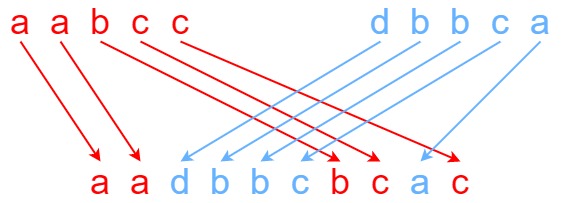
Input: s1 = "aabcc", s2 = "dbbca", s3 = "aadbbcbcac" Output: true Explanation: One way to obtain s3 is: Split s1 into s1 = "aa" + "bc" + "c", and s2 into s2 = "dbbc" + "a". Interleaving the two splits, we get "aa" + "dbbc" + "bc" + "a" + "c" = "aadbbcbcac". Since s3 can be obtained by interleaving s1 and s2, we return true.
Example 2:
Input: s1 = "aabcc", s2 = "dbbca", s3 = "aadbbbaccc" Output: false Explanation: Notice how it is impossible to interleave s2 with any other string to obtain s3.
Example 3:
Input: s1 = "", s2 = "", s3 = "" Output: true
Constraints:
0 <s1.length, s2.length <= 100=0 <s3.length <= 200=s1,s2, ands3consist of lowercase English letters.
Follow up: Could you solve it using only O(s2.length) additional
memory space?
※ 2.17.7.1. Constraints and Edge Cases
<list constraints, input limits, or tricky edge cases here>
※ 2.17.7.2. My Solution (Code)
※ 2.17.7.2.1. v1: guided
1: class Solution: 2: │ def isInterleave(self, s1: str, s2: str, s3: str) -> bool: 3: │ │ m, n = len(s1), len(s2) 4: │ │ if (m + n) != len(s3): 5: │ │ │ return False 6: │ │ │ 7: │ │ dp = [[False] * (n + 1) for _ in range(m + 1)] 8: │ │ dp[0][0] = True 9: │ │ 10: │ │ # init first column (only s1): 11: │ │ for i in range(1, m + 1): 12: │ │ │ dp[i][0] = dp[i - 1][0] and s1[i - 1] == s3[i - 1] 13: │ │ │ 14: │ │ # init first row (only s2): 15: │ │ for j in range(1, n + 1): 16: │ │ │ dp[0][j] = dp[0][j - 1] and s2[j - 1] == s3[j - 1] 17: │ │ │ 18: │ │ # fill the rest: 19: │ │ for i in range(1, m + 1): 20: │ │ │ for j in range(1, n + 1): 21: │ │ │ │ dp[i][j] = ( 22: │ │ │ │ │ dp[i - 1][j] 23: │ │ │ │ │ and s1[i - 1] == s3[i + j - 1] 24: │ │ │ │ ) or ( 25: │ │ │ │ │ dp[i][j - 1] 26: │ │ │ │ │ and s2[j - 1] == s3[i + j - 1] 27: │ │ │ │ ) 28: │ │ │ │ 29: │ │ return dp[m][n]
- Intuition Recap
- Each cell
dp[i][j]asks: “Can I form the prefix of s3 of lengthi + jusing prefixes of s1 and s2 of lengthsiandjrespectively?” - You build solutions to subproblems based on smaller prefixes, working up to the full strings.
- Each cell
※ 2.17.7.2.2. v2: space optimised
from v1, we notice that dp[i][j] is caculated as such:
1: │ │ │ │ dp[i][j] = ( 2: │ │ │ │ │ dp[i - 1][j] # prev one matched 3: │ │ │ │ │ and s1[i - 1] == s3[i + j - 1] # matching char 4: │ │ │ │ ) or ( 5: │ │ │ │ │ dp[i][j - 1] # prev one matched 6: │ │ │ │ │ and s2[j - 1] == s3[i + j - 1] # maching char 7: │ │ │ │ )
So it only depends on:
- previous row, same column (we filled top to bottom)
- same row, previous column (we fill left to right)
So we can stick to the inner loop being left to right.
Important: When updating dp, iterate over j from left to right (0 to n) because dp[j] corresponds to dp[i][j] and previous state dp[j-1] is still available in this iteration (the current fella).
so we get the following:
1: class Solution: 2: │ def isInterleave(self, s1: str, s2: str, s3: str) -> bool: 3: │ │ m, n = len(s1), len(s2) 4: │ │ if (m + n) != len(s3): 5: │ │ │ return False 6: │ │ │ 7: │ │ dp = [False] * (n + 1) # in terms of s2 8: │ │ # trivial fill: nothingness is trivially true 9: │ │ dp[0] = True 10: │ │ 11: │ │ # trivial fill first row, init first row values: 12: │ │ # round 1 fill first row 13: │ │ for j in range(1, n + 1): 14: │ │ │ dp[j] = dp[j - 1] and s2[j - 1] == s3[j - 1] 15: │ │ │ 16: │ │ # for prefixes of s1, this is what we are doing inclusions on 17: │ │ for i in range(1, m + 1): 18: │ │ │ 19: │ │ │ # updates dp[0] for column zero (only s1 to be used as prefix to form s3) 20: │ │ │ dp[0] = dp[0] and s1[i - 1] == s3[i - 1] 21: │ │ │ 22: │ │ │ for j in range(1, n + 1): 23: │ │ │ │ dp[j] = ( 24: │ │ │ │ │ │ ( # case A: last letter in s1 matches last letter in s3 25: │ │ │ │ │ │ │ dp[j] 26: │ │ │ │ │ │ │ and s1[i - 1] == s3[i + j - 1] 27: │ │ │ │ │ │ ) 28: │ │ │ │ │ │ or 29: │ │ │ │ │ │ ( # case B: last letter in s2 matches last letter in s3 30: │ │ │ │ │ │ │ dp[j - 1] 31: │ │ │ │ │ │ │ and s2[j - 1] == s3[i + j - 1] 32: │ │ │ │ │ │ ) 33: │ │ │ │ ) 34: │ │ │ │ 35: │ │ return dp[n]
Explanation of the flattening logic:
dp[j]in the inner loop corresponds todp[i][j]in the 2D version.- Before the inner loop starts,
dp[j]holds values from the previous row(i-1). - We update
dp[j]using those old values anddp[j-1](from current row so far). - This update order and rolling over 1D dp ensure the logic is preserved exactly.
Slightly cleaner:
1: class Solution: 2: │ def isInterleave(self, s1: str, s2: str, s3: str) -> bool: 3: │ │ m, n = len(s1), len(s2) 4: │ │ if m + n != len(s3): 5: │ │ │ return False 6: │ │ │ 7: │ │ # dp[j] = can s3[:i+j] be formed by s1[:i] and s2[:j] 8: │ │ dp = [False] * (n + 1) 9: │ │ dp[0] = True # empty s1/s2 → empty s3 10: │ │ 11: │ │ # Initialize first row (i = 0, use only s2's prefix) 12: │ │ for j in range(1, n + 1): 13: │ │ │ dp[j] = dp[j - 1] and s2[j - 1] == s3[j - 1] 14: │ │ │ 15: │ │ # Process each prefix length of s1 16: │ │ for i in range(1, m + 1): 17: │ │ │ # Update dp[0] for column 0 (use only s1's prefix) 18: │ │ │ dp[0] = dp[0] and s1[i - 1] == s3[i - 1] 19: │ │ │ 20: │ │ │ for j in range(1, n + 1): 21: │ │ │ │ dp[j] = ( 22: │ │ │ │ │ (dp[j] and s1[i - 1] == s3[i + j - 1]) or 23: │ │ │ │ │ (dp[j - 1] and s2[j - 1] == s3[i + j - 1]) 24: │ │ │ │ ) 25: │ │ │ │ 26: │ │ return dp[n]
※ 2.17.7.3. My Approach/Explanation
Think about the problem as building s3 by taking characters from s1 or s2.
Use indices to track positions.
Can use dp table or recursive helpers.
※ 2.17.7.4. My Learnings/Questions
when I’m completely stuck, it’s important to think of the meanings of the operations, which will give us some useful properties to exploit.
In this case, there’s a need to know what “interleaving” means here.
Interleaving means that any char from s3 comes from either s1 or s2 and if can’t be there, then it’s not possible to build it up.
<what did you learn? any uncertainties or questions?>
※ 2.17.8. ⭐️ [132] Distinct Subsequences (115) hard subsequences dp
Given two strings s and t, return the number of distinct subsequences of s which equals t.
The test cases are generated so that the answer fits on a 32-bit signed integer.
Example 1:
Input: s = "rabbbit", t = "rabbit" Output: 3 Explanation: As shown below, there are 3 ways you can generate "rabbit" from s. rabbbit rabbbit rabbbit
Example 2:
Input: s = "babgbag", t = "bag" Output: 5 Explanation: As shown below, there are 5 ways you can generate "bag" from s. babgbag babgbag babgbag babgbag babgbag
Constraints:
1 <s.length, t.length <= 1000=sandtconsist of English letters.
※ 2.17.8.1. Constraints and Edge Cases
※ 2.17.8.2. My Solution (Code)
※ 2.17.8.2.1. v0: almost there but some accuracy mistakes
1: class Solution: 2: │ def numDistinct(self, s: str, t: str) -> int: 3: │ │ n, m = len(s), len(t) 4: │ │ 5: │ │ if n < m: 6: │ │ │ return 0 7: │ │ │ 8: │ │ # dp[i][j] shall represent the number of ways to make t[:j] from s[:i] 9: │ │ dp = [[0] * (n + 1) for _ in range(m + 1)] 10: │ │ 11: │ │ dp[0][0] = 1 12: │ │ 13: │ │ # for the target: 14: │ │ for i in range(m + 1): 15: │ │ │ target = t[:i] 16: │ │ │ # for the source 17: │ │ │ for j in range(n + 1): 18: │ │ │ │ if s[j] == t[i]: 19: │ │ │ │ │ dp[i][j] = dp[i][j - 1] + 1 20: │ │ │ │ else: 21: │ │ │ │ │ dp[i][j] = dp[i][j - 1] 22: │ │ │ │ │ 23: │ │ return dp[m][n]
Problems:
- the counting of the matching case is not correct
if the characters match, we should be doing
dp[i][j] = dp[i][j-1] + dp[i-1][j-1]:
dp[i][j-1]= number of ways to formt[:i]froms[:j-1](not usings[j-1])dp[i-1][j-1]= number of ways to formt[:i-1]froms[:j-1](usings[j-1]to matcht[i-1])
※ 2.17.8.2.2. v1: improved the accuracy
1: class Solution: 2: │ def numDistinct(self, s: str, t: str) -> int: 3: │ │ n, m = len(s), len(t) 4: │ │ 5: │ │ if n < m: 6: │ │ │ return 0 7: │ │ │ 8: │ │ # dp[i][j] shall represent the number of ways to make t[:j] from s[:i] 9: │ │ dp = [[0] * (n + 1) for _ in range(m + 1)] 10: │ │ 11: │ │ # all the 0 length can be fromed from any prefix of s 12: │ │ for j in range(n + 1): 13: │ │ │ dp[0][j] = 1 14: │ │ │ 15: │ │ # for the target: 16: │ │ for i in range(1, m + 1): 17: │ │ │ # for the source 18: │ │ │ for j in range(1, n + 1): 19: │ │ │ │ if s[j - 1] == t[i - 1]: 20: │ │ │ │ │ # on last char match, we take: 21: │ │ │ │ │ # A: ways without current char in s (dp[i][j-1]) 22: │ │ │ │ │ # B: ways using the current matching char (dp[i-1][j-1]) 23: │ │ │ │ │ dp[i][j] = dp[i][j - 1] + \ 24: │ │ │ │ │ │ │ │ dp[i - 1][ j - 1] # ans to the prev letter 25: │ │ │ │ else: 26: │ │ │ │ │ dp[i][j] = dp[i][j - 1] 27: │ │ │ │ │ 28: │ │ return dp[m][n]
※ 2.17.8.2.3. v2: flattened from 2D to 1D:
When filling dp[i][j], we only ever reference:
dp[i][j-1] → current row, previous column
dp[i-1][j-1] → previous row, previous column
That means:
Column j depends only on column j-1 in this iteration (row i) and from the previous iteration (row i-1).
We can keep just one row and update it in place if we go backwards in i to avoid overwriting dp[i-1] before it’s used.
So we can just do 1D version:
1: class Solution: 2: │ def numDistinct(self, s: str, t: str) -> int: 3: │ │ n, m = len(s), len(t) 4: │ │ if n < m: 5: │ │ │ return 0 6: │ │ │ 7: │ │ dp = [0] * (m + 1) 8: │ │ dp[0] = 1 # empty t matches any prefix of s 9: │ │ 10: │ │ for ch in s: 11: │ │ │ for i in range(m, 0, -1): # update backwards 12: │ │ │ │ if t[i-1] == ch: 13: │ │ │ │ │ dp[i] += dp[i-1] 14: │ │ │ │ │ 15: │ │ return dp[m]
※ 2.17.8.3. My Approach/Explanation
so this seems to be a matter of moving two pointers and counting the number of chars within to see whether or not we can create it.
So the outer loop shall be the thing that we’re trying to create ( the target ) and the inner loop should be all the sources.
※ 2.17.8.4. My Learnings/Questions
so close, the main intuition is in the recurrence relation which looks like this:
\[ dp[i][j] = \underbrace{dp[i][j-1]}_{\text{ignore } s[j-1]} + \underbrace{dp[i-1][j-1]}_{\text{use } s[j-1] \text{ to match } t[i-1]} \]
here’s more context on it:
Show/Hide Md CodeGreat question! Let's unpack why the recurrence for the **Distinct Subsequences** problem is: $$ dp[i][j] = dp[i][j - 1] + dp[i - 1][j - 1] $$ and **not** something like `dp[i][j-1] + 1`. ### What does `dp[i][j]` represent? - `dp[i][j]` = the **number of distinct subsequences** of `s[:j]` that equals `t[:i]`. - In other words, how many ways can we form the first `i` characters of `t` from the first `j` characters of `s`. ### Intuition when characters match (`s[j-1] == t[i-1]`) Consider the situation where the current characters are equal: - One way to get `t[:i]` from `s[:j]` is to **ignore** the current character `s[j-1]` — so the count is the same as `dp[i][j-1]`. - The other way is to **use** this current character `s[j-1]` to match `t[i-1]` — so the count is the number of ways to form the prefix `t[:i-1]` from `s[:j-1]`, which is `dp[i-1][j-1]`. Thus: $$ dp[i][j] = \underbrace{dp[i][j-1]}_{\text{ignore } s[j-1]} + \underbrace{dp[i-1][j-1]}_{\text{use } s[j-1] \text{ to match } t[i-1]} $$ No extra `+1` is added because we're **counting the number of subsequences**, not just checking existence or adding one occurrence. ### Why not `dp[i][j-1] + 1`? - `dp[i][j-1]` is already a count of how many ways to form `t[:i]` **without using** `s[j-1]`. - **Adding 1 would mean just one additional subsequence**, which is incorrect because **there could be many ways** of matching `t[:i-1]` in `s[:j-1]` to pair with `s[j-1]`. - Instead, you add all the ways from `dp[i-1][j-1]`. ### What about when characters don't match? If `s[j-1] != t[i-1]`, the current character in `s[j-1]` can't contribute to subsequences matching `t[:i]`. So: $$ dp[i][j] = dp[i][j-1] $$ Meaning we only have the subsequences formed without using the current character. ### A simple example Suppose: - `s = "babgbag"` - `t = "bag"` Let's look at a small step where the characters at `s[j-1]` and `t[i-1]` match (both 'g'): - Count subsequences matching `t[:i]` by: │ - Ignoring this 'g' in `s` (so count remains `dp[i][j-1]`) │ - Using this 'g' to match the current character in `t` (we add `dp[i-1][j-1]` possible ways) │ So you **accumulate all ways** from both possibilities. ### Summary: - The recurrence counts **all subsequences**, so you sum counts from ignoring or using the current character. - It is a **sum of counts** of subsequences, **not a sum plus one**. - Hence: $$ dp[i][j] = dp[i][j - 1] + dp[i - 1][j - 1] $$ when characters match. Let me know if you'd like me to illustrate with a worked-out numeric example on a small string!
※ 2.17.9. [133] Edit Distance (72) subsequences prefix_matching
Given two strings word1 and word2, return the minimum number of
operations required to convert word1 to word2.
You have the following three operations permitted on a word:
- Insert a character
- Delete a character
- Replace a character
Example 1:
Input: word1 = "horse", word2 = "ros" Output: 3 Explanation: horse -> rorse (replace 'h' with 'r') rorse -> rose (remove 'r') rose -> ros (remove 'e')
Example 2:
Input: word1 = "intention", word2 = "execution" Output: 5 Explanation: intention -> inention (remove 't') inention -> enention (replace 'i' with 'e') enention -> exention (replace 'n' with 'x') exention -> exection (replace 'n' with 'c') exection -> execution (insert 'u')
Constraints:
0 <word1.length, word2.length <= 500=word1andword2consist of lowercase English letters.
※ 2.17.9.1. Constraints and Edge Cases
Nothing fancy
※ 2.17.9.2. My Solution (Code)
※ 2.17.9.2.1. v0 wrong because of execution issues
this is actually the correct structure and intuition, the mistakes here will be useful to define the common mistakes here.
1: class Solution: 2: │ def minDistance(self, word1: str, word2: str) -> int: 3: │ │ n, m = len(word1), len(word2) 4: │ │ if not n and not m: 5: │ │ │ return 0 6: │ │ │ 7: │ │ # dp[i][j] shows min number of operations to use to convert word1[:i] to word2[:j] 8: │ │ dp = [[float('inf')] * (n + 1) for _ in range(m + 1)] 9: │ │ # trivial base cases: 10: │ │ dp[0][0] = 0 11: │ │ for i in range(m + 1): 12: │ │ │ dp[i][0] = 1 # deletion only for the first column in dp table 13: │ │ │ 14: │ │ for j in range(n + 1) : 15: │ │ │ dp[0][j] = 1 # insertion only for the first row in the dp table 16: │ │ │ 17: │ │ for j in range(1, m + 1): 18: │ │ │ # target = word2[:j] 19: │ │ │ for i in range(1, n + 1): 20: │ │ │ │ # if it's the same, do nothing: 21: │ │ │ │ if word1[i - 1] == word2[j - 1]: 22: │ │ │ │ │ dp[i][j] = dp[i - 1][j - 1] 23: │ │ │ │ else: 24: │ │ │ │ │ # we can do an insertion from the previous 25: │ │ │ │ │ insertion_case = dp[i - 1][j] + 1 26: │ │ │ │ │ replace_case = dp[i][j] + 1 27: │ │ │ │ │ removal_case = dp[i + 1][j] + 1 28: │ │ │ │ │ dp[i][j] = min(insertion_case, replace_case, removal_case) 29: │ │ │ │ │ 30: │ │ return dp[m][n]
confusion on table dimensions and what represents what. the init for the dp table is wrong in this attempt:
Show/Hide Diff Code-dp = [[float('inf')] * (n + 1) for _ in range(m + 1)] # gives (m + 1) x (n + 1) shape +dp = [[float('inf')] * (m + 1) for _ in range(n + 1)] # gives (n + 1) x (m + 1) shape
- so we are correct when we say that
dp[i][j]represent edit distance to convertword1[:i]toword2[:j] dpis size(n+1) x (m+1)(rows \(\rightarrow\)len(word1), cols \(\rightarrow\)len(word2)).dp[i][j]: min operations to convert firstichars of word1 to firstjchars of word2.
- so we are correct when we say that
base case init is wrong:
Show/Hide Python Code1: dp[0][0] = 0 2: for i in range(m + 1): 3: │ dp[i][0] = 1 # should be i, not 1 because we need to make that many edits 4: for j in range(n + 1): 5: │ dp[0][j] = 1 # should be j, not 1 because we need to make that many edits
- what to loop over for the main business logic is depending on what the variables mean
If
dp[i][j]means conversion ofword1[:i]toword2[:j], then:the proper definitions for the recurrence should be:
Show/Hide QuoteUsing proper definitions: Insertions: convert word1[:i-1] to word2[:j], then insert word1[i-1]: dp[i][j] = dp[i-1][j] + 1
Deletions: convert word1[:i] to word2[:j-1], then delete or insert a char: dp[i][j] = dp[i][j-1] + 1
Replacements: convert word1[:i-1] to word2[:j-1], then replace word1[i-1] with word2[j-1]: dp[i][j] = dp[i-1][j-1] + 1
- Outer loop over i in 1..n
Inner loop over j in 1..m
Show/Hide Python Code1: │ │ for i in range(1, n + 1): 2: │ │ │ for j in range(1, m + 1): 3: │ │ │ │ # if it's the same, do nothing: 4: │ │ │ │ if word1[i - 1] == word2[j - 1]: 5: │ │ │ │ │ dp[i][j] = dp[i - 1][j - 1] 6: │ │ │ │ else: 7: │ │ │ │ │ insertion_case = dp[i - 1][j] + 1 8: │ │ │ │ │ replace_case = dp[i][j] + 1 # this is wrong, it should be dp[i - 1][j - 1] + 1 9: │ │ │ │ │ removal_case = dp[i + 1][j] + 1 # this is wrong because i + 1 may be out of bounds, it should dp[i - 1][j] + 1 10: │ │ │ │ │ dp[i][j] = min(insertion_case, replace_case, removal_case)
※ 2.17.9.2.2. v1: corrected dp table filling
1: class Solution: 2: │ def minDistance(self, word1: str, word2: str) -> int: 3: │ │ n, m = len(word1), len(word2) 4: │ │ 5: │ │ # dp[i][j] shows min number of operations to use to convert word1[:i] to word2[:j] 6: │ │ dp = [[0] * (m + 1) for _ in range(n + 1)] 7: │ │ 8: │ │ for i in range(n + 1): 9: │ │ │ dp[i][0] = i # delete all from word1 to get empty word2 10: │ │ │ 11: │ │ for j in range(m + 1) : 12: │ │ │ dp[0][j] = j # insert all to convert empty word1 to word2[:j] 13: │ │ │ 14: │ │ for i in range(1, n + 1): 15: │ │ │ for j in range(1, m + 1): 16: │ │ │ │ if word1[i - 1] == word2[j - 1]: 17: │ │ │ │ │ dp[i][j] = dp[i - 1][j - 1] 18: │ │ │ │ else: 19: │ │ │ │ │ insertion = dp[i][j - 1] + 1 20: │ │ │ │ │ deletion = dp[i - 1][j] + 1 21: │ │ │ │ │ replacement = dp[i - 1][j - 1] + 1 22: │ │ │ │ │ dp[i][j] = min(insertion, deletion, replacement) 23: │ │ │ │ │ 24: │ │ return dp[n][m]
※ 2.17.9.2.3. v2: space optimised with 2 rolling rows
1: class Solution: 2: │ def minDistance(self, word1: str, word2: str) -> int: 3: │ │ n, m = len(word1), len(word2) 4: │ │ if n < m: 5: │ │ │ # ensure n >= m to use less space 6: │ │ │ return self.minDistance(word2, word1) 7: │ │ │ 8: │ │ previous_row = list(range(m + 1)) 9: │ │ current_row = [0] * (m + 1) 10: │ │ 11: │ │ for i in range(1, n + 1): 12: │ │ │ current_row[0] = i 13: │ │ │ for j in range(1, m + 1): 14: │ │ │ │ if word1[i - 1] == word2[j - 1]: 15: │ │ │ │ │ current_row[j] = previous_row[j - 1] 16: │ │ │ │ else: 17: │ │ │ │ │ insert_op = current_row[j - 1] + 1 18: │ │ │ │ │ delete_op = previous_row[j] + 1 19: │ │ │ │ │ replace_op = previous_row[j - 1] + 1 20: │ │ │ │ │ current_row[j] = min(insert_op, delete_op, replace_op) 21: │ │ │ │ │ 22: │ │ │ # swap them 23: │ │ │ previous_row, current_row = current_row, previous_row 24: │ │ │ 25: │ │ │ 26: │ │ return previous_row[m]
※ 2.17.9.3. My Approach/Explanation
Yet another subsequence, we try to take a source and make it fit to a destination word.
The idea here is to take two slices and build from source slice to destination slice.
This will allow us to build from small to big.
Seems like a pretty common pattern for subsequences.
※ 2.17.9.4. My Learnings/Questions
This problem requires global lookahead and subproblem reuse, satisfying optimal substructure.
Greedy approaches fail due to lack of greedy-choice property.
DP with carefully chosen states (prefix lengths of the two words) captures maximal subsolutions and overlaps.
- careful on the sources of error described above.
※ 2.17.9.5. [Optional] Additional Context
Pretty happy with myself for this, just the execution details that is lacking.
※ 2.17.9.6. Retro
※ 2.17.9.6.1.
I think it’s VERY IMPORTANT to define the meanings of i and j and the table dimension meanings when writing out the answer so that we don’t end up wasting time rethinking that part or worse, getting confused.
the determining of filling order and state transitions also becomes easier.
※ 2.17.10. [134] ⭐️ Burst Balloons (312) redo hard interval_DP divide_and_conquer think_in_reverse matmul_dp_pattern
You are given n balloons, indexed from 0 to n - 1. Each balloon is
painted with a number on it represented by an array nums. You are
asked to burst all the balloons.
If you burst the i=^{=th} balloon, you will get
nums[i - 1] * nums[i] * nums[i + 1] coins. If i - 1 or i + 1 goes
out of bounds of the array, then treat it as if there is a balloon with
a 1 painted on it.
Return the maximum coins you can collect by bursting the balloons wisely.
Example 1:
Input: nums = [3,1,5,8] Output: 167 Explanation: nums = [3,1,5,8] --> [3,5,8] --> [3,8] --> [8] --> [] coins = 3*1*5 + 3*5*8 + 1*3*8 + 1*8*1 = 167
Example 2:
Input: nums = [1,5] Output: 10
Constraints:
n =nums.length=1 <n <= 300=0 <nums[i] <= 100=
※ 2.17.10.1. Constraints and Edge Cases
<list constraints, input limits, or tricky edge cases here>
※ 2.17.10.2. My Solution (Code)
※ 2.17.10.2.1. v1: guided Interval DP in \(O(n^3)\) time
1: class Solution: 2: │ def maxCoins(self, nums: List[int]) -> int: 3: │ │ nums = [1] + nums + [1] # we add the edge padding, the numbers are trivial because it's all multiplication 4: │ │ 5: │ │ n = len(nums) 6: │ │ dp = [[0] * n for _ in range(n)] 7: │ │ 8: │ │ # length is the interval length from small to big (2 to n) 9: │ │ for length in range(2, n): 10: │ │ │ for left in range(n - length): 11: │ │ │ │ right = left + length 12: │ │ │ │ # where k = last pop idx: 13: │ │ │ │ for k in range(left + 1, right): 14: │ │ │ │ │ left_interval, right_interval = dp[left][k], dp[k][right] 15: │ │ │ │ │ this_burst = nums[left] * nums[k] * nums[right] 16: │ │ │ │ │ coins = left_interval + this_burst + right_interval 17: │ │ │ │ │ 18: │ │ │ │ │ dp[left][right] = max(coins, dp[left][right]) 19: │ │ │ │ │ 20: │ │ # NOTE: the 1s are trivial because it's multiplication 21: │ │ return dp[0][n - 1]
Tricks:
- the adding of the edge 1s are very clever, it’s harmless because it’s product and we don’t need to explicitly handle the edges
- the use of length outer loop makes is a neat, the
rightis just derived based onlengthandleft
※ 2.17.10.3. My Approach/Explanation
I’m a little lost on this one.
Some observations:
- bursting is essentially making the value to 1. So any time we do any other bursting, we just expand left and right until we get something that is NOT one.
- I can’t think of a subproblem version for this though.
- I think a greedy solution does NOT work because of what happens after the bursting, the collating need not be locally optima that leads to global optima.
※ 2.17.10.4. My Learnings/Questions
Optimal Approach:
DP setup:
dp[i][j]is the maximum coins obtained by bursting balloons between indicesiandj\(\rightarrow\)nums[i + 1]tonums[j + 1]
DP recurrence:
for each interval \((i, j)\), we burst balloons \(k\) as the last balloon in the interval where \(i < k < j\)
If we burst
klast, the coins gained aredp[i][k] + dp[k][j] + (nums[i] * nums[k] * nums[j])Where
dp[i][k]anddp[k][j]are the results of bursting balloons in subintervals to the left and right of kDP base cases:
For intervals of length 2 (i.e., adjacent balloons),
dp[i][j] = 0since there are no balloons betweeniandj.Table filling directionality: We fill up dp from smaller intervals to larger intervals.
Trick: Think in reverse:
Instead of choosing which balloon to burst first, think about which balloon to burst last in a given subinterval.
Why?
When bursting the last balloon in an interval, its neighbors are fixed (outside the interval), so calculating coins is easier.
You divide the problem into smaller subproblems by splitting the balloons into left and right subintervals around the last balloon to burst.
※ 2.17.11. DONE [135] Regular Expression Matching (10) hard regex_matching 2D_string_matching
- CLOSING NOTE
- CLOSING NOTE
This is nice, it’s a classic example
Given an input string s and a pattern p, implement regular
expression matching with support for '.' and '*' where:
'.'Matches any single character.'*'Matches zero or more of the preceding element.
The matching should cover the entire input string (not partial).
Example 1:
Input: s = "aa", p = "a" Output: false Explanation: "a" does not match the entire string "aa".
Example 2:
Input: s = "aa", p = "a*" Output: true Explanation: '*' means zero or more of the preceding element, 'a'. Therefore, by repeating 'a' once, it becomes "aa".
Example 3:
Input: s = "ab", p = ".*" Output: true Explanation: ".*" means "zero or more (*) of any character (.)".
Constraints:
1 <s.length <= 20=1 <p.length <= 20=scontains only lowercase English letters.pcontains only lowercase English letters,'.', and'*'.- It is guaranteed for each appearance of the character
'*', there will be a previous valid character to match.
※ 2.17.11.1. Constraints and Edge Cases
<list constraints, input limits, or tricky edge cases here>
※ 2.17.11.2. My Solution (Code)
※ 2.17.11.2.1. v0 : failed, wrong understanding of *
1: class Solution: 2: │ def isMatch(self, s: str, p: str) -> bool: 3: │ │ n, m = len(s), len(p) 4: │ │ 5: │ │ pattern_info = [(False, None) for _ in range(m)] 6: │ │ for idx in range(1, m): 7: │ │ │ if p[idx] == "*": 8: │ │ │ │ (_, val) = pattern_info[idx] 9: │ │ │ │ pattern_info[idx] = (True, val) 10: │ │ │ │ 11: │ │ # dp size is (n + 1) x (m + 1) 12: │ │ # dp[i][j] represents bool whether s[:i] can be represented by p[:j] 13: │ │ dp = [[False] * (m + 1) for _ in range(n + 1)] 14: │ │ 15: │ │ # trivial base cases: for s[0] all can be represented by the pattern trivially 16: │ │ for j in range(m + 1): 17: │ │ │ dp[0][j] = True 18: │ │ │ 19: │ │ # now we build: 20: │ │ for i in range(1, n + 1): 21: │ │ │ # target = s[:i] 22: │ │ │ for j in range(1, m + 1): 23: │ │ │ │ direct_match = s[i - 1] == p[j - 1] 24: │ │ │ │ any_char_match = p[j - 1] == '.' 25: │ │ │ │ has_preceeding, preceding_val = pattern_info[j - 1] 26: │ │ │ │ valid_preceeding = has_preceeding and s[i - 1] == preceding_val 27: │ │ │ │ 28: │ │ │ │ dp[i][j] = direct_match or any_char_match or valid_preceeding 29: │ │ │ │ 30: │ │ return dp[n][m]
Problems:
- the handling of
*is only a one character lookback. so star can be:representing 0 occurrence of preceding char:
dp[i][j] = dp[i][j - 2]- if preceding char matches
s[i - 1]then star can represent one or more: ifp[j - 2] =s[i - 1] or p[j - 2]= '.'then we can do dp[i][j] |= dp[i - 1][j]
※ 2.17.11.2.2. v1: guided
※ 2.17.11.3. My Approach/Explanation
<briefly explain your reasoning, algorithm, and why you chose it>
※ 2.17.11.4. My Learnings/Questions
<what did you learn? any uncertainties or questions?>
※ 2.17.11.5. Prompt for GPT Evaluation
Please do the following:
- Evaluate the correctness of my solution. Are there any logical or edge case errors?
- Analyze the time and space complexity of my code.
- Suggest improvements in code style, efficiency, or clarity.
- Compare my approach to the optimal solution (if different).
- Provide a sample optimal solution (if mine is not optimal).
- Point out any Pythonic (or language-specific) improvements.
Are there any completely different approaches to this problem?
- e.g something that uses a completely different data structure
If so, then help me gain the intuition for it and show the code clearly
- Answer my specific questions (if any are listed above).
※ 2.17.11.6. Prompt for GPT Evaluation (with Greedy)
Please do the following:
- Evaluate the correctness of my solution. Are there any logical or edge case errors?
- Analyze the time and space complexity of my code.
- Suggest improvements in code style, efficiency, or clarity.
- Compare my approach to the optimal solution (if different).
- Provide a sample optimal solution (if mine is not optimal).
- Point out any Pythonic (or language-specific) improvements.
Are there any completely different approaches to this problem?
- e.g something that uses a completely different data structure
If so, then help me gain the intuition for it and show the code clearly
- Answer my specific questions (if any are listed above).
ALso help me evaluate this in the context of greedy algorithms, ensuring that a good framework of presenting this problem into a greedy algo is given / understood.
※ 2.17.11.7. Prompt for GPT Evaluation (with DP)
Please do the following:
- Evaluate the correctness of my solution. Are there any logical or edge case errors?
- Analyze the time and space complexity of my code.
- Suggest improvements in code style, efficiency, or clarity.
- Compare my approach to the optimal solution (if different).
- Provide a sample optimal solution (if mine is not optimal).
- Point out any Pythonic (or language-specific) improvements.
Are there any completely different approaches to this problem?
- e.g something that uses a completely different data structure
If so, then help me gain the intuition for it and show the code clearly
- Answer my specific questions (if any are listed above).
ALso help me evaluate this in the context of greedy algorithms, ensuring that a good framework of presenting this problem into a greedy algo is given / understood.
Additionally, use my notes for Dynamic Programming and use the recipes that are here.
Recipe to define a solution via DP
[Generate Naive Recursive Algo]
Characterise the structure of an optimal solution \(\implies\) what are the subproblems? \(\implies\) are they independent subproblems? \(\implies\) how many subproblems will there be?
- Recursively define the value of an optimal solution \(\implies\) does this have the overlapping sub-problems property? \(\implies\) what’s the cost of making a choice? \(\implies\) how many ways can I make that choice?
- Compute value of an optimal solution
- Construct optimal solution from computed information Defining things
- Optimal Substructure:
A problem exhibits “optimal substructure” if an optimal solution to the problem contains within it optimal solutions to subproblems.
Elements of Dynamic Programming: Key Indicators of Applicability [1] Optimal Sub-Structure Defining “Optimal Substructure” A problem exhibits optimal substructure if an optimal solution to the problem contains within it optimal solutions to sub-problems.
- typically a signal that DP (or Greedy Approaches) will apply here.
- this is something to discover about the problem domain Common Pattern when Discovering Optimal Substructure
solution involves making a choice e.g. choosing an initial cut in the rod or choosing what k should be for splitting the matrix chain up
\(\implies\) making the choice also determines the number of sub-problems that the problem is reduced to
- Assume that the optimal choice can be determined, ignore how first.
- Given the optimal choice, determine what the sub-problems looks like \(\implies\) i.e. characterise the space of the subproblems
- keep the space as simple as possible then expand
typically the substructures vary across problem domains in 2 ways:
[number of subproblems]
how many sub-problems does an optimal solution to the original problem use?
- rod cutting:
# of subproblems = 1(of size n-i) where i is the chosen first cut lengthmatrix split:
# of subproblems = 2(left split and right split)[number of subproblem choices]
how many choices are there when determining which subproblems(s) to use in an optimal solution. i.e. now that we know what to choose, how many ways are there to make that choice?
- rod cutting: # of choices for i = length of first cut,
nchoices- matrix split: # of choices for where to split (idx k) =
j - iNaturally, this is how we analyse the runtime:
# of subproblems * # of choices @ each sub-problem- Reason to yourself if and how solving the subproblems that are used in an optimal solution means that the subproblem-solutions are also optimal. This is typically done via the
cut-and-paste argument.Caveat: Subproblems must be
independent
- “independent subproblems”
- solution to one subproblem doesn’t affect the solution to another subproblem for the same problem
example: Unweighted Shortest Path (independent subproblems) vs Unweighted Longest Simple Path (dependent subproblems)
Consider graph \(G = (V,E)\) with vertices \(u,v \notin V\)
- Unweighted shortest path: we want to find path \(u\overset{p}{\leadsto}v\) then we can break it down into subpaths \(u\overset{p1}{\leadsto}w\overset{p2}{\leadsto}v\) (optimal substructure). If path, p, is optimal from \(u\leadsto{v}\) then p1 must be shortest path from \(u\leadsto{w}\) and likewise p2 must be shortest path from \(w\leadsto{v}\) (cut-and-paste argument) Here, we know that the subproblems are independent.
- Unweighted Longest Simple Path: the subproblems can have paths that overlap (not subproblem overlap), hence it’s not independent because the vertices that appear can appear in the solution to the second subproblem
Terminology: Optimal substruture vs optimal solution optimal substructure is a property that enables efficient computation of the optimal value, while the solution is the specific configuration that yields that optimal value
You’re right that in dynamic programming algorithms for optimization problems, the goal is usually to find an optimal solution rather than the unique optimal solution. Here’s how the optimal substructure and the actual solution differ:
### Optimal Substructure
The optimal substructure refers to the property that the optimal solution to a problem can be constructed from the optimal solutions to its subproblems. This means that if we know the optimal solutions to the subproblems, we can efficiently determine the optimal solution to the overall problem.
For example, in the rod cutting problem, if we know the maximum revenue for rods of length 1 to n-1, we can efficiently determine the maximum revenue for a rod of length n by considering cutting the rod at each possible length and taking the maximum revenue.
### The Solution
The actual solution, on the other hand, refers to the specific configuration or set of choices that yields the optimal value. In the rod cutting problem, the solution would be the specific way to cut the rod that results in the maximum revenue.
The key difference is that the optimal substructure allows us to efficiently compute the optimal value, but it doesn’t necessarily specify the exact solution. There may be multiple solutions that yield the same optimal value.
For example, in the rod cutting problem, there may be multiple ways to cut the rod that result in the same maximum revenue. The optimal substructure allows us to efficiently compute the maximum revenue, but it doesn’t specify which particular cutting configuration to choose.
So in summary, the optimal substructure is a property that enables efficient computation of the optimal value, while the solution is the specific configuration that yields that optimal value. Dynamic programming algorithms leverage the optimal substructure to efficiently compute the optimal value, but the actual solution may not be uniquely determined.
Citations: [1] https://library.fiveable.me/key-terms/programming-for-mathematical-applications/optimal-substructure [2] https://afteracademy.com/blog/optimal-substructure-and-overlapping-subproblems/ [3] https://www.geeksforgeeks.org/optimal-substructure-property-in-dynamic-programming-dp-2/ [4] https://labuladong.gitbook.io/algo-en/i.-dynamic-programming/optimalsubstructure [5] https://stackoverflow.com/questions/33563230/optimal-substructure-in-dynamic-programing [6] https://en.wikipedia.org/wiki/Optimal_substructure [7] https://www.cs.cmu.edu/~15451-f22/lectures/lec09-dp1.pdf [8] https://www.javatpoint.com/optimal-substructure-property
[2] Overlapping Sub-Problems
- DP should be disambiguated from Divide & Conquer:
- for Divide&Conquer, choosing a division point generates brand new problems that likely don’t overlap
- for DP, the space of sub-problems is small and hence if done purely recursively, the same operations get computed multiple times
[Practical point] Reconstructing an optimal solution Since one way to look at DP is table-filling, we typically have:
- table of costs
- table of optimal choices
the table of optimal choices can be built from the table of costs, but we want to avoid recalculating the optimal choices
Memoisation as an alternative
- the textbook used sees this as an alternative and memoised tables as the aux DS for recursive, top-down approaches
- memoisation also exploits the observation that the space of the subproblems is small and hence overlapping
Common Misconceptions Here are some common misconception, based on what perplexity says
Based on the search results, here are some of the common misconceptions that learners have about dynamic programming:
## 1. Misconceptions about the Definition and Purpose of Dynamic Programming
- Thinking that recursion and dynamic programming are explicitly different concepts[3].
- Believing that dynamic programming is exclusively used to solve optimization problems[3].
## 2. Misconceptions about the Optimal Substructure Property
- Assuming that the optimal solution to a problem can be constructed from any combination of optimal solutions to its subproblems, rather than specific optimal solutions to the right subproblems[1][2].
- Thinking that the optimal solution to a problem can be constructed from optimal solutions to unrelated subproblems[4].
## 3. Misconceptions about Memoization and Tabulation
- Failing to recognize that memoization (top-down) and tabulation (bottom-up) are two different implementation strategies for dynamic programming[1][2].
- Believing that memoization always involves recursion and tabulation always involves iteration[1][2].
## 4. Misconceptions about the Filling Order of the DP Table
- Assuming that the DP table must always be filled in a specific order (e.g., always from small to big cases), without understanding that the order depends on the problem’s dependencies and constraints[1][2][4].
## 5. Misconceptions about the Relationship between Subproblems
- Thinking that the solutions to all subproblems are needed to solve the original problem, rather than understanding that only specific optimal solutions to the right subproblems are needed[1][2].
## 6. Misconceptions about the Efficiency of Dynamic Programming
- Believing that dynamic programming always leads to polynomial-time algorithms, without understanding that it can sometimes only slightly improve the exponential-time complexity[4].
Understanding and addressing these common misconceptions can help learners develop a more accurate and comprehensive understanding of dynamic programming and its applications.
Citations: [1] https://dl.acm.org/doi/10.1145/3159450.3159528 [2] https://dl.acm.org/doi/abs/10.1145/3159450.3159528 [3] https://ics.uci.edu/~mikes/papers/Student_Misconceptions_Dynamic_Programming.pdf [4] https://www.cs.cmu.edu/~15451-f22/lectures/lec09-dp1.pdf [5] https://www.reddit.com/r/compsci/comments/er05hn/help_me_wrap_my_head_around_dynamic_programming/ [6] https://yourbasic.org/algorithms/dynamic-programming-explained/ [7] https://stackoverflow.com/questions/33563230/optimal-substructure-in-dynamic-programing [8] https://lec.inf.ethz.ch/DA/2020/slides/daLecture13.en.pdf
Greedy Algos vs DP When comparing greedy strategies and dynamic programming (DP), it’s essential to understand how they differ in methodology, application, and the nature of the problems they solve. Both approaches involve identifying optimal substructures, but they apply this concept in distinct ways. Here’s a detailed disambiguation based on the search results:
### 1. Definition and Approach
- Greedy Strategy:
- A greedy algorithm makes the most optimal choice at each step with the hope that these local optimum choices will lead to a global optimum solution. It does not consider the overall impact of the current choice on future decisions.
- Greedy algorithms are typically simpler and faster to implement, as they do not require storing results of subproblems. However, they do not guarantee an optimal solution for all problems.
- Dynamic Programming:
- Dynamic programming is a technique used to solve complex problems by breaking them down into simpler subproblems. It is based on the principles of optimal substructure and overlapping subproblems.
- DP guarantees an optimal solution by considering all possible cases and storing the results of subproblems to avoid redundant computations. This can lead to higher time and space complexity compared to greedy algorithms.
### 2. Optimal Substructure
- Greedy Algorithms:
- Greedy algorithms rely on the greedy choice property, which means that a locally optimal choice leads to a globally optimal solution. However, this property does not hold for all problems, which is why greedy algorithms may fail to find the optimal solution in some cases.
- Dynamic Programming:
- Dynamic programming explicitly uses the optimal substructure property, where an optimal solution to a problem can be constructed from optimal solutions of its subproblems. DP ensures that all relevant subproblems are considered, leading to a guaranteed optimal solution.
### 3. Subproblem Reuse
- Greedy Strategy:
- Greedy algorithms typically do not reuse solutions to subproblems. Each decision is made independently based on the current state without revisiting previous choices.
- Dynamic Programming:
- DP explicitly solves and caches solutions to overlapping subproblems. This reuse of subproblem solutions is a key feature of dynamic programming, allowing for efficient computation.
### 4. Complexity and Efficiency
- Greedy Algorithms:
- Greedy algorithms are generally more efficient in terms of time complexity due to their straightforward approach. They often run in linear or logarithmic time, depending on the problem.
- They are suitable for problems where local optimization leads to global optimization, such as in minimum spanning trees or certain shortest path problems.
- Dynamic Programming:
- DP can be less efficient than greedy algorithms in terms of time complexity, especially if every possible solution is computed. However, proper use of memoization can mitigate this.
- DP is applicable to problems with overlapping subproblems and optimal substructure, such as the Fibonacci sequence, longest common subsequence, or knapsack problems.
### 5. Examples
- Greedy Algorithms:
- Common examples include:
- Fractional Knapsack Problem: Where you can take fractions of items.
- Minimum Spanning Tree: Algorithms like Prim’s and Kruskal’s.
- Huffman Coding: For optimal prefix codes.
- Dynamic Programming:
- Common examples include:
- 0/1 Knapsack Problem: Where you cannot take fractions of items.
- Longest Common Subsequence: Finding the longest subsequence present in both sequences.
- Matrix Chain Multiplication: Finding the most efficient way to multiply a given sequence of matrices.
### Conclusion
In summary, while both greedy strategies and dynamic programming involve the concept of optimal substructure, they differ significantly in their approach to problem-solving. Greedy algorithms make decisions based on local optimality without revisiting previous choices, whereas dynamic programming systematically considers all possible subproblems and their solutions to ensure a globally optimal result. Understanding these differences allows for better problem-solving strategies and the appropriate application of each method based on the problem’s characteristics.
Citations: [1] https://www.boardinfinity.com/blog/greedy-vs-dp/ [2] https://www.shiksha.com/online-courses/articles/difference-between-greedy-and-dynamic-programming-blogId-158053 [3] https://www.interviewbit.com/blog/difference-between-greedy-and-dynamic-programming/ [4] https://stackoverflow.com/questions/16690249/what-is-the-difference-between-dynamic-programming-and-greedy-approach [5] https://www.geeksforgeeks.org/greedy-approach-vs-dynamic-programming/ [6] https://byjus.com/gate/difference-between-greedy-approach-and-dynamic-programming/ [7] https://www.cs.cmu.edu/~15451-f22/lectures/lec09-dp1.pdf [8] https://ics.uci.edu/~mikes/papers/Student_Misconceptions_Dynamic_Programming.pdf
General Takeaways Bottom-up vs Top-Down
- we can use a subproblem graph to show the relationship with the subproblems ==> diff b/w bottom up and top-down is how these deps are handled (recursive-called or soundly iterated with a proper direction)
- aysymptotic runtime is pretty similar since both solve similar \(\Omega(n^{2})\)
- Bottom up:
- basically considers order at which the subproblems are solved
- because of the ordered way of solving the smaller sub-problems first, there’s no need for recursive calls and code can be iterative entirely
- so no overhead from function calls
- no chance of stack overflow
- benefits from data-locality
- a way to see the vertices of the subproblem graph such that the subproblems y-adjacent to a given subproblem x is solved before subproblem x is solved
※ 2.17.11.8. [Optional] Additional Context
<e.g., “I struggled with X”, “I want to know about alternative algorithms”, etc.>
※ 2.17.11.9. Retros
※ 2.17.11.9.1.
This is great. The general structure makes sense. I am ready to do blinds now.
I think the combining cases can be a little deceptive here for the wildcard part:
1: # elif p[j - 1] == '*': 2: # # case 1: zero occurence of preceding char: 3: # is_valid_zero_case = dp[i][j - 2] 4: # # case 2: one or more occurrence if preceding char matches s[i - 1] 5: # is_matching_preceeding_char = dp[i][j] or p[j - 2] == s[i - 1] or p[j - 2] == '.' 6: 7: # dp[i][j] = is_valid_zero_case or is_matching_preceeding_char 8: 9: elif p[j - 1] == '*': 10: │ # zero occurrence 11: │ dp[i][j] = dp[i][j - 2] 12: │ # one or more 13: │ if p[j - 2] == s[i - 1] or p[j - 2] == '.': 14: │ │ dp[i][j] = dp[i][j] or dp[i - 1][j]
※ 2.17.12. [Depth Blind 1] Word Break II (140) hard failed
Given a string s and a dictionary of strings wordDict, add spaces in
s to construct a sentence where each word is a valid dictionary word.
Return all such possible sentences in any order.
Note that the same word in the dictionary may be reused multiple times in the segmentation.
Example 1:
Input: s = "catsanddog", wordDict = ["cat","cats","and","sand","dog"] Output: ["cats and dog","cat sand dog"]
Example 2:
Input: s = "pineapplepenapple", wordDict = ["apple","pen","applepen","pine","pineapple"] Output: ["pine apple pen apple","pineapple pen apple","pine applepen apple"] Explanation: Note that you are allowed to reuse a dictionary word.
Example 3:
Input: s = "catsandog", wordDict = ["cats","dog","sand","and","cat"] Output: []
Constraints:
1 <s.length <= 20=1 <wordDict.length <= 1000=1 <wordDict[i].length <= 10=sandwordDict[i]consist of only lowercase English letters.- All the strings of
wordDictare unique. - Input is generated in a way that the length of the answer doesn’t exceed 105.
※ 2.17.12.0.1. Constraints and Edge Cases
<list constraints, input limits, or tricky edge cases here>
※ 2.17.12.0.2. My Solution (Code)
I failed this, I wasted 15min just beign scared.
Realised that the question should be directly solved after the initial analysis instead of us trying to consistently pattern match into a canonical problem type.
I got till here.
I know that a backtrack approach has aspects of itself that needs to be super charged by external DSes.
I think it’s actually BOTH a 2D dp as well as a trie to make the “dp[i][j] = True if s[i:j] is a legit word” part faster.
1: class Solution: 2: │ def wordBreak(self, s: str, wordDict: List[str]) -> List[str]: 3: │ │ # likely need an aux ds to tell us if some range of i,j is a valid word or not 4: │ │ # then we need to pick where we can place the spaces, we need to keep track of the path. So this feels like a decision tree traversal and I'm likely going to do some sort of dfs / backtracking for this 5: │ │ 6: │ │ # 1. aux ds first, using dp dp[i][j] whether s[i + 1: j + 1] (slice) is a legit word or not 7: │ │ # ther'es no substructure here. 8: │ │ wordSet = set(wordDict) # O(1) lookups on this. 9: │ │ n = len(s) 10: │ │ 11: │ │ # I could use trie for representing the worddict, the dictionary can be a map from word to end node? 12: │ │ # dp[i][j]: is s[i:j] a legit word i will be values of left, j will be values for right 13: │ │ dp = [ [False] * (n + 1) for j in range(n + 1)] 14: │ │ dp[0][0] = True # trivially 15: │ │ for i in range(1, n + 1): 16: │ │ │ for j in range(1, n + 1): 17: │ │ │ 18: │ │ sentences = [] 19: │ │ 20: │ │ 21: │ │ def backtrack(path, char_count, left): 22: │ │ │ if left == n: 23: │ │ │ │ if char_count == n: 24: │ │ │ │ │ # path built so it's a valid sentenck: 25: │ │ │ │ │ sentences.append(path) 26: │ │ │ │ else: 27: │ │ │ │ │ return # deadend 28: │ │ │ │ │ 29: │ │ │ for left in range(n): 30: │ │ │ │ # right exclusive for slicing 31: │ │ │ │ # IMPROVE: i should have some kind of next possible index that I can emplace a space from left. 32: │ │ │ │ for right in range(n + 1): 33: │ │ │ │ │ candidate = s[left:right] 34: │ │ │ │ │ if candidate in wordSet: # I could pause here 35: │ │ │ │ │ │ # choose it: 36: │ │ │ │ │ │ path.append(s[left:right]) 37: │ │ │ │ │ │ backtrack(path, char_count + 1, right) 38: │ │ │ │ │ │ # backtrack on it 39: │ │ │ │ │ │ path.pop() 40: │ │ │ │ │ else: 41: │ │ │ │ │ │ continue 42: │ │ │ return 43: │ │ │ 44: │ │ backtrack([], 0, 0) 45: │ │ 46: │ │ return sentences
1: from functools import cache 2: 3: class Solution: 4: │ def wordBreak(self, s: str, wordDict: List[str]) -> List[str]: 5: │ │ wordSet = set(wordDict) 6: │ │ 7: │ │ @cache 8: │ │ def backtrack(start_idx): 9: │ │ │ # end-cases: 10: │ │ │ if start_idx == len(s): 11: │ │ │ │ return [""] # trivially, we return a sentence with empty string 12: │ │ │ │ 13: │ │ │ res = [] # sentences to form starting with start_idx 14: │ │ │ for end in range(start_idx + 1, len(s) + 1): 15: │ │ │ │ word = s[start_idx:end] 16: │ │ │ │ if not word in wordSet: 17: │ │ │ │ │ continue 18: │ │ │ │ │ 19: │ │ │ │ # we can backtrack now: 20: │ │ │ │ choices = backtrack(end) 21: │ │ │ │ for sub in choices: 22: │ │ │ │ │ if sub: 23: │ │ │ │ │ │ res.append(f"{word} {sub}") 24: │ │ │ │ │ else: # current word is last word 25: │ │ │ │ │ │ res.append(word) # this is the last word in the sentence 26: │ │ │ return res 27: │ │ │ 28: │ │ return backtrack(0)
The main idea here is that backtrack(start) actually returns values. In this case all the sub-sentences from the slice of string s[start:]
1: from typing import List 2: from functools import cache 3: 4: class Solution: 5: │ def wordBreak(self, s: str, wordDict: List[str]) -> List[str]: 6: │ │ n = len(s) 7: │ │ wordset = set(wordDict) 8: │ │ 9: │ │ dp = [False] * (n + 1) 10: │ │ dp[0] = True 11: │ │ valid_starts = [[] for _ in range(n + 1)] 12: │ │ 13: │ │ for i in range(1, n + 1): 14: │ │ │ for j in range(i): 15: │ │ │ │ if dp[j] and s[j:i] in wordset: 16: │ │ │ │ │ dp[i] = True 17: │ │ │ │ │ valid_starts[i].append(j) 18: │ │ │ │ │ 19: │ │ if not dp[n]: 20: │ │ │ return [] 21: │ │ │ 22: │ │ @cache 23: │ │ def backtrack(end): 24: │ │ │ if end == 0: 25: │ │ │ │ return [""] 26: │ │ │ sentences = [] 27: │ │ │ for start in valid_starts[end]: 28: │ │ │ │ word = s[start:end] 29: │ │ │ │ prefixes = backtrack(start) 30: │ │ │ │ for prefix in prefixes: 31: │ │ │ │ │ if prefix: 32: │ │ │ │ │ │ sentences.append(f"{prefix} {word}") 33: │ │ │ │ │ else: 34: │ │ │ │ │ │ sentences.append(word) 35: │ │ │ return sentences 36: │ │ │ 37: │ │ return backtrack(n)
- we carry on with backtrack approach
※ 2.17.12.0.3. My Approach/Explanation
※ 2.17.12.0.4. My Learnings/Questions
- how not to waste the first 15min just trying to iterate through my bag of tricks.
※ 2.17.12.0.5. [Optional] Additional Context
Yes this was a failure, but for a first blind done properly, I think there are some mini wins to be happy about:
- the phrasing of the main problem as a backtrack and accumulation is important and I got that right.
I realise that the immediate prior context of me having done DP questions ended up making me try to force fit the bottom up DP approach.
This was rough, I think it’s alright to focus on solving the problem instead of trying to use a hammer (trick from bag of tricks) to solve everything that I see.
<e.g., “I struggled with X”, “I want to know about alternative algorithms”, etc.>
※ 2.17.13. [Depth Blind 2] Number of Unique Good Subsequences (1987) hard failed counting 2_state_tracking
You are given a binary string binary. A subsequence of binary is
considered good if it is not empty and has no leading zeros (with
the exception of "0").
Find the number of unique good subsequences of binary.
- For example, if
binary = "001", then all the good subsequences are["0", "0", "1"], so the unique good subsequences are"0"and"1". Note that subsequences"00","01", and"001"are not good because they have leading zeros.
Return the number of unique good subsequences of binary. Since the
answer may be very large, return it modulo 10=^{=9}= + 7=.
A subsequence is a sequence that can be derived from another sequence by deleting some or no elements without changing the order of the remaining elements.
Example 1:
Input: binary = "001" Output: 2 Explanation: The good subsequences of binary are ["0", "0", "1"]. The unique good subsequences are "0" and "1".
Example 2:
Input: binary = "11" Output: 2 Explanation: The good subsequences of binary are ["1", "1", "11"]. The unique good subsequences are "1" and "11".
Example 3:
Input: binary = "101" Output: 5 Explanation: The good subsequences of binary are ["1", "0", "1", "10", "11", "101"]. The unique good subsequences are "0", "1", "10", "11", and "101".
Constraints:
1 <binary.length <= 10=5binaryconsists of only =’0’=s and =’1’=s.
※ 2.17.13.1. Constraints and Edge Cases
<list constraints, input limits, or tricky edge cases here>
※ 2.17.13.2. My Solution (Code)
※ 2.17.13.2.1. V1: guided
1: from collections import Counter 2: class Solution: 3: │ def numberOfUniqueGoodSubsequences(self, binary: str) -> int: 4: │ │ MOD = (10 ** 9) + 7 5: │ │ 6: │ │ if len(binary) == 1: 7: │ │ │ return 1 8: │ │ │ 9: │ │ end0, end1, has0 = 0, 0, False 10: │ │ 11: │ │ for c in binary: 12: │ │ │ if c == '1': 13: │ │ │ │ # can append to the end of everything that we have already encountered 14: │ │ │ │ end1 = ((end0 + end1) + 1) % MOD 15: │ │ │ else: 16: │ │ │ │ has0 = True 17: │ │ │ │ # can only append '0' to those that end with 1: 18: │ │ │ │ # since end0 all the time will NEVER have a violator (so never someone with leading 0s) then we can add to all the numbers in end0 and all the numbers in end1 19: │ │ │ │ end0 = (end0 + end1) % MOD 20: │ │ │ │ 21: │ │ return ((1 if has0 else 0) + end0 + end1) % MOD
the no leading zero rule means that we need to track the subsequences that end with 1 and 0 separately
so say we keep
end0, end1- it’s like 2 state handling:
if curr bit is 1: then we can append it at the end of everything we have encountered so far.
we can start a new subsequence with just 1 also
so we have the transition equation:
end1 = ((end0 + end1) + 1) % MODthe +1 here is because of the fact that we can also use 1 as a sole subsequence
if curr bit is 0: then we can only append to the 1s (else we risk violating the leading 0 rule):
end0 = (end0 + end1) % MODwhy this? because we know at any point in time end0 will just have
Here’s a slightly cleaner version
1: class Solution: 2: │ def numberOfUniqueGoodSubsequences(self, binary: str) -> int: 3: │ │ MOD = 10**9 + 7 4: │ │ count_end_with_0 = 0 5: │ │ count_end_with_1 = 0 6: │ │ has_zero = False 7: │ │ 8: │ │ for ch in binary: 9: │ │ │ if ch == '1': 10: │ │ │ │ # Append '1' to all subsequences (ending with 0 or 1) + start new subsequence '1' 11: │ │ │ │ count_end_with_1 = (count_end_with_0 + count_end_with_1 + 1) % MOD 12: │ │ │ else: 13: │ │ │ │ # Append '0' only to subsequences ending with '1' 14: │ │ │ │ has_zero = True 15: │ │ │ │ count_end_with_0 = (count_end_with_0 + count_end_with_1) % MOD 16: │ │ │ │ 17: │ │ # sum subsequences ending with 0 and 1 plus subsequence "0" if exists 18: │ │ return (count_end_with_0 + count_end_with_1 + (1 if has_zero else 0)) % MOD
※ 2.17.13.3. My Approach/Explanation
- we know that it’s going to be a huge number, so we can’t expect any aux ds approach that is space heavy
- it ended up being so much simpler (just a counting problem) than expected.
- just because it’s DP doesn’t mean we have to handle so many complex tricks. This is also technically DP because we are doing state tracking as we sweep through an array.
※ 2.17.13.4. My Learnings/Questions
Just a note about the module and why it works: it’s because addition and multiplication commute with taking modulo; there’s no loss of information
Show/Hide Md CodeThe reason you can keep taking modulo at every step (e.g., in `count_end_with_0 = (count_end_with_0 + count_end_with_1) % MOD`) without losing any information is due to a fundamental property of modular arithmetic: **addition and multiplication commute with taking modulo**.[1][2][3] ## Why Partial Sums Modulo Work For any modulus $$ m $$: - $$ (a + b) \bmod m = ((a \bmod m) + (b \bmod m)) \bmod m $$ - $$ (a \times b) \bmod m = ((a \bmod m) \times (b \bmod m)) \bmod m $$ This means that no matter how large the intermediate sum or product gets, *as long as you take modulo at each addition or multiplication, the final result modulo $$m$$ will be correct* — you never impact the remainder.[2][1] **Intuition:** Suppose you are adding up (potentially huge) numbers. All you care about is the remainder (modulo some value). Any excess above multiples of that modulus will always "wrap around" the modulus, so keeping only the current remainder is sufficient.[3][1][2] ### Application to Your Code The subsequence counting logic may generate astronomical numbers — but storing and updating only the current value modulo $$10^9 + 7$$ is enough, because modulo arithmetic guarantees correctness of the result's remainder. When you sum at the end, as long as each intermediate value was modulo'd, the final sum modulo $$10^9 + 7$$ matches what an exact (but potentially massive) calculation would yield.[1][2][3] **No information about the answer modulo $$m$$ is lost by discarding higher-order multiples of $$m$$ at each step.** This is what makes modulo arithmetic so robust for "counting" DP methods and combinatorial questions in programming contests and number theory.[2][3][1] [1](https://www2.math.upenn.edu/~mlazar/math170/notes06.pdf) [2](https://brilliant.org/wiki/modular-arithmetic/) [3](https://en.wikipedia.org/wiki/Modular_arithmetic) [4](https://www.youtube.com/watch?v=gJtw0c3Lo6E) [5](https://www.geeksforgeeks.org/engineering-mathematics/modular-arithmetic/) [6](https://davidaltizio.web.illinois.edu/ModularArithmetic.pdf) [7](https://calcworkshop.com/number-theory/modular-arithmetic/) [8](https://www.math.purdue.edu/~arapura/algebra/algebra8.pdf) [9](https://sites.math.rutgers.edu/~zeilberg/essays683/renault.html)
I kept thinking of a way to get this done but couldn’t come up with ANY sort of DP solution. The final answer seems so simple, it’s just a 2 state handling.
The fact that the bot recommended this under DP hard problems made me try to come up with fancy DP tricks for this. If I came in blind to the topic at hand, I think I would have thought more simply.
I think for this, as long as we try to think of bit distribution, we’ll always end up with the 2 state counting solution.
※ 2.17.13.5. [Optional] Additional Context
It’s alright, first 2 blinds were not idea but it’s alright.
※ 2.18. Bit Manipulation
| Headline | Time | ||
|---|---|---|---|
| Total time | 2:11 | ||
| Bit Manipulation | 2:11 | ||
| [136] Single Number (136) | 0:09 | ||
| [137] Number of 1 Bits (191) | 0:13 | ||
| [138] Counting Bits (338) | 0:21 | ||
| [139] Reverse Bits (190) | 0:30 | ||
| [140] Missing Number (268) | 0:03 | ||
| [141] ⭐️Sum of Two Integers (371) | 0:22 | ||
| [142] ⭐️Reverse Integer (7) | 0:33 |
※ 2.18.1. General Notes
※ 2.18.1.1. Fundamentals
We are interested in efficient techniques for working with integers at the bit level. These range from basic bit tests and modifications, to more advanced techniques for counting bits, reversing bits, branchless min/max, and bitwise power-of-2 checks.
※ 2.18.1.1.1. Summary
Bitwise Operations
Bit manipulation uses AND (
&), OR (|), XOR (^), NOT (~), as well as left (\(<<\)) and right (\(>>\)) shifts to efficiently operate on binary representations of data.Common Tricks
Includes checks like “is number a power of 2?”, “count the number of set bits”, “swap values without temp variable”, and more.
Branch-free programming
Recommends writing expressions that avoid branching (if-else) for potential speed advantages, especially in critical code.
Sign Handling
Hacks for branchless computation of sign, absolute value, min/max.
Some caveats on portability between python and C
Some hacks rely on two’s complement representation and how right shift of signed values works, which is standardized in Python but not always portable in C.
- python compatibility
- bitwise operators work the same as in C
char operations, need to use
ord()andchr(). Consider the “lowercase character” trick:C:
'A' | ' 'gives the lowercase'c'python :
chr(ord('A') | ord(' '))likewise for the uppercase trick where we use bitwise AND instead of bitwise OR
- python integers:
has no representation for unsigned int
are arbitrary precision, they are signed and auto-grow. So if we need 32-bit unsigned behaviour, we have to mask it:
value & 0xFFFFFFFF- Doing right-shifting for sign extension works for negative ints in python.
Works for Python’s negative ints, but always confirm behavior, especially for emulating C-style fixed-width truncation if needed.
In C, C++, Java:
0xFFFFFFFFis-1as a signed 32-bit integer (all bits set). As unsigned, it’s4,294,967,295.In Python: integers are unbounded, so masking with
0xFFFFFFFFensures results are as if you’d done a 32-bit operation (ignores auto-extensions)- we’d have to use pythonic ways of doing boolean operations vs C
e.g. checking if a number is a power of two:
Show/Hide Python Code│ │ # in python: │ │ (v != 0) and ((v & (v - 1)) == 0) │ │ # in c: │ │ # v && !(v & (v - 1))
Classic Use Cases
State Compression
We can use bits to represent subsets or masks e.g. DP with bitmasking
Bit Counting (popcount):
We can use this for subset enumeration, generating combinations…
- Power of 2 Checks
Branchless Tricks
Faster min/max, absolute value, sign, swaps, conditional operations
- Bitmask-based enumeration
Used when the total state fits within 32 or 64 bits
Low Level Data transformations
Reversing bits, byte swapping
Leetcode Use Cases
Some problems:
Trick/Pattern Description Example Leetcode Problem popcount, bitmask DP Subset/superset DP, combinatorics 698 (Partition to K Equal Sum), 464 (Can I Win) xor-trick Find unique/odd elements using XOR 136 (Single Number), 260 (Single Number III) get_lowest_set_bitEfficient set manipulation 89 (Gray Code), 201 (Bitwise AND of Numbers Range) min/max/abs branchless Optimize performance, avoid branch (rare explicit Leetcode, but common in contests) state compression Boolean matrix to bitmask 691 (Stickers to Spell Word) reverse bits Reverse binary representation 190 (Reverse Bits)
DP on Subsets:
Traveling Salesman Problem (TSP), longest path covering all nodes, “Minimum Path Cover”, “Partition into Subsets”
Unique Elements/Single Numbers:
XOR tricks for “find element that appears once/twice”, a staple in Leetcode
Mask DP:
For small n (\(n \leq 20\)), DP state is often stored as
dp[mask]where mask encodes visited states/itemsSet Cover / Subset Enumeration:
Enumerate all possible subsets via bitmask integer (\(\approx 2^{n}\))
Bitwise operations for
“AND/OR/XOR of array/subset”
Odd/Even Parity Checks:
XOR over all bits, used for error detection (parity), game theory
Reverse Bits/Bytes:
Used in problems testing endianness, bit reversal (see Leetcode 190)
Gray Code:
Useful in problems asking about minimal transitions in binary
Branchless min/max/abs:
Efficient calculations without conditionals
Parallel Counting/Rank:
Fast ways to count how many bits set up to a certain position
※ 2.18.1.1.2. Understanding bit masking
mental model: A mask is a stencil: imagine laying a piece of paper with holes (1s) over your data — only bits where the mask is 1 “show through.”
Masking is like using a filter over binary data, making it essential for low-level programming and algorithmic tricks.
Use the width of the mask to match the portion of the value you’re interested in.
bit width
Match your mask’s bit-width to your intent:
A mask is typically in hexadecimal \(\implies\) each digit represents 4 bits.
So,
- 0xFF \(\rightarrow\) 8 bits
- 0xFFFF \(\rightarrow\) 16 bits
- 0xFFFFFFFF \(\rightarrow\) 32 bits
practical use cases of bitmasking Extracting Flags:
status & 0x0Fkeeps bottom 4 bits (flags).Packing Data:
Store multiple boolean or small-integer values in a single variable.
Clearing Bits:
value & ~masksets bits to 0 wherever mask is 1.Boundary Enforcement:
Masking user input, forcing to a certain bit-width (
x & 0xFF).
※ 2.18.1.1.3. Recipes:
The way ASCII encoding has been done using numerical code-points, the use of code points for spaces and underscores allow us to do these bit hacks:
convert English chars to lowercase using
|chr(ord('a') | ord(' ')) # gives 'a', no changechr(ord('A') | ord(' ')) # gives 'a'; upper to lowerconvert English chars to uppercase using
&chr(ord('b') & ord(' ')) # gives 'B' make uppercasechr(ord('B') & ord(' ')) # gives 'B' no changetoggle casing of English chars using
^chr(ord('d') ^ ord(' ')) # gives 'D'; toggle lower to upperchr(ord('D') ^ ord(' ')) # gives 'd' # toggle upper to lower
Memory Manipulations
we can swap two integers without using a temporary variable.
Show/Hide Python Code1: a = 1, b = 2; 2: a ^= b; 3: b ^= a; 4: a ^= b;
QQ: this seems to only be for integers, floats don’t work (this is because the bitwise XOR is not defined for floats, only for ints)
- Incrementing / Decrementing:
both of these work because the numbers in python are represented using 2s complement, which allows us to do some automatic arithmetic on it:
- to increment we do
n = -~nthe~flips every bit ofnthen the negation will add 1 ton; works because of the 2s-complement representation of numbers - to decrement we do
n = ~-nso-ncomputes the 2s-complement negative then taking the bitwise NOT subtracts 1 fromn
- to increment we do
comparing signs,
is_opposite? using 2-s complement manipulations It utilizes the sign bit of two’s complement encoding.The highest bit in integer encoding is the sign bit:
negative numbers have a sign bit of 1, non-negative numbers have a sign bit of 0.
Using the properties of XOR, you can determine if two numbers have opposite signs
is_opposite = bool((x ^ y) < 0) # where x and y are two different numbers
- check the \(N^{th}\) bit:
(x >> n) & 1right shift by n positions and check AND 1 - set the \(N^{th}\) bit:
x | (1 << n)left shift 1 by n positions and OR it with x - clear \(N^{th}\) bit:
x & ~(1 << n)left shift 1 by n then flip it to be zero then use that to AND with x to clear the nth bit - toggle \(N^{th}\) bit:
x ^ (1 << n)left shift 1 by n then xor it with x
There’s a bunch of ways to do popcount:
[best] use the builtin:
n.bit_count() # where n is an intthis needs python 3.10+
- [old] stringify then count 1s:
bin(n).count('1') [old, long] bitwise clear the lowest set bit iteratively:
Show/Hide Python Code1: def popcount(x): 2: │ c = 0 3: │ while x: 4: │ │ x &= x - 1 5: │ │ c += 1 6: │ return c
x & -x
x & (x - 1)
1: mask = some_mask 2: sub = mask 3: while sub: 4: │ # use sub 5: │ sub = (sub - 1) & mask
n & (n - 1) to remove LSB (Brian Kernighan’s algorithm)- Uses:
Eliminating the last (LSB) 1 in the binary representation of number
ncore logic is that
n - 1will always remove the last 1 and turn all trailing 0s into 1s. Then, performing the&operation with n will turnonly the last 1 into 0Calculating Hamming Weight (number of set bits)
This way of removing LSB is useful for counting hamming weight.
Keep removing MSB 1 until the whole number is 0.
However, there are better ways to get hamming weight in python (see sections above).
Show/Hide Python Code1: class Solution: 2: │ def hammingWeight(self, n: int) -> int: 3: │ │ res = 0 4: │ │ while n != 0: 5: │ │ │ n = n & (n - 1) 6: │ │ │ res += 1 7: │ │ return res
Determine if a number is a power of 2
A number is a power of two if its binary representation contains only one ’1’. So if we remove LSB 1, then it should be 0
Show/Hide Python Code1: class Solution: 2: │ def isPowerOfTwo(self, n: int) -> bool: 3: │ │ if n <= 0: 4: │ │ │ return False 5: │ │ │ 6: │ │ return (n & (n - 1)) == 0
a ^ a = 0
A number XORed with itself results in 0, i.e., a ^ a = 0; a number XORed with 0 results in itself, i.e., a ^ 0 = a
LeetCode Problem 136 “Single Number”
For this problem, XOR all the numbers.
Pairs of numbers will result in 0, and the single number XORed with 0 will still be itself.
Therefore, the final XOR result is the element that appears only once:
1: class Solution: 2: │ def singleNumber(self, nums: List[int]) -> int: 3: │ │ res = 0 4: │ │ 5: │ │ for num in nums: 6: │ │ │ # num xor-ed with 0 will give itself, pairs will cancel out 7: │ │ │ res ^= num 8: │ │ │ 9: │ │ return res
268. Missing Number | LeetCode
the bithack version hinges on the fact that XOR is commutative and associative.
Consider adding an index and then to each element we have indices that correspond to its equal index:

After doing this, you can see that all indices and elements form pairs, except for the missing element. Now, if we find the single index 2, we find the missing element.
By XORing all elements and indices, paired numbers will cancel out to 0, leaving the single element, achieving our goal
1: class Solution: 2: │ def missingNumber(self, nums: List[int]) -> int: 3: │ │ n = len(nums) 4: │ │ res = 0 5: │ │ # first XOR with the new added index 6: │ │ res ^= n 7: │ │ # XOR with other elements and indices 8: │ │ for i in range(n): 9: │ │ │ res ^= i ^ nums[i] 10: │ │ return res
Situations:
- when the array length is power of 2
Do:
index & (len(arr) - 1) as the accessor idx
so it’s arr[index & (len(arr) - 1)]
Simply put, the bitwise operation & (len(arr) - 1) can replace the modulo operation % len(arr), providing better performance.
Now the question arises, if you are continuously index++, you achieve circular iteration. But can you still achieve the effect of a circular array if you continuously index–?
The answer is, if you use the % modulo method, when index becomes less than 0, the modulo result can also be negative, requiring special handling. However, with the & bitwise operation, index won’t become negative and can still work normally:
※ 2.18.1.2. Tricks
This whole topic is all so hacky, this “Tricks” section is going to be more specific to the questions I will encounter.
※ 2.18.1.3. Sources of Error
※ 2.18.2. [136] Single Number (136) classic pair_cancellation_via_XOR
Given a non-empty array of integers nums, every element appears
twice except for one. Find that single one.
You must implement a solution with a linear runtime complexity and use only constant extra space.
Example 1:
Input: nums = [2,2,1]
Output: 1
Example 2:
Input: nums = [4,1,2,1,2]
Output: 4
Example 3:
Input: nums = [1]
Output: 1
Constraints:
1 <nums.length <= 3 * 10=4-3 * 10=^{=4}= <= nums[i] <= 3 * 10=4- Each element in the array appears twice except for one element which appears only once.
※ 2.18.2.1. Constraints and Edge Cases
- can only use constant space, linear runtime
※ 2.18.2.2. My Solution (Code)
※ 2.18.2.2.1. v0: optimal approach using XORs
1: class Solution: 2: │ """ 3: │ Finds the element that appears only once in a list where each element appears twice, except for one. 4: │ Uses XOR to cancel pairs. 5: │ """ 6: │ 7: │ def singleNumber(self, nums: List[int]) -> int: 8: │ │ res = 0 9: │ │ 10: │ │ for num in nums: 11: │ │ │ # num xor-ed with 0 will give itself, pairs will cancel out 12: │ │ │ res ^= num 13: │ │ │ 14: │ │ return res
※ 2.18.2.3. My Approach/Explanation
- everyone has a pair except one \(\implies\) we can exploit the XOR properties:
- commutative: we can shift things around, it’s alright same result so each number will cancel itself out when we XOR it, except for the one that is single.
※ 2.18.2.4. My Learnings/Questions
- Yay use of XORs!
- If every number appears three times except one (LeetCode 137), you need bit counting. But for this problem, XOR is the unbeatable method.
※ 2.18.2.5. [Optional] Additional Context
I knew of this since this is a classic problem.
※ 2.18.3. [137] Number of 1 Bits (191) hamming_weight popcount
Given a positive integer n, write a function that returns the number
of set bits in its binary representation (also known as the
Hamming weight).
Example 1:
Input: n = 11
Output: 3
Explanation:
The input binary string 1011 has a total of three set bits.
Example 2:
Input: n = 128
Output: 1
Explanation:
The input binary string 10000000 has a total of one set bit.
Example 3:
Input: n = 2147483645
Output: 30
Explanation:
The input binary string 1111111111111111111111111111101 has a total of thirty set bits.
Constraints:
1 <n <= 2=31= - 1=
Follow up: If this function is called many times, how would you optimize it?
※ 2.18.3.1. Constraints and Edge Cases
Nothing fancy here.
- Handles
n = 0(returns 0) and all positive integers up to2^31 - 1, as per constraints.
※ 2.18.3.2. My Solution (Code)
※ 2.18.3.2.1. v0: optimal count the number of LSB that is set
1: class Solution: 2: │ def hammingWeight(self, n: int) -> int: 3: │ │ counter = 0 4: │ │ while n != 0: 5: │ │ │ n &= (n - 1) 6: │ │ │ counter += 1 7: │ │ │ 8: │ │ return counter
- complexity analysis:
- Time Complexity:
- \(O(k)\), where \(k\) is the number of set bits in the input n.
- This is more efficient than looping over every bit if n is very sparse (few set bits).
- \(O(k)\), where \(k\) is the number of set bits in the input n.
- Space Complexity:
- \(O(1)\), constant space (just one counter and local variables).
- Time Complexity:
※ 2.18.3.2.2. v1: exploiting python idiomatic built-ins
1: def hammingWeight(self, n: int) -> int: 2: │ return bin(n).count('1')
may not be good for sparse numbers because it goes through every bit because of this counting approach.
Actually there’s a new stdlib function that we can use for python 3.10+
1: return n.bit_count()
※ 2.18.3.2.3. v2: using a bitmask, iterating over all bits
1: def hammingWeight(self, n: int) -> int: 2: │ count = 0 3: │ for i in range(32): 4: │ │ count += n & 1 # 1 if that bit is set, else 0 5: │ │ n >>= 1 # right-shift for next consideration 6: │ return count
Intuition: Check and count each bit from least to most significant.
※ 2.18.3.3. My Approach/Explanation
We use the bit trick that extracts the LSB that is set from a number ( n & (n - 1) )
※ 2.18.3.4. My Learnings/Questions
- reminder that the LSB removal is pretty useful
extra learning: C has builtin hardware accelerated functions for this
For very large numbers or repeated calls, perhaps leverage hardware-accelerated functions (like C’s
__builtin_popcount), though Python standard libraries do not offer this natively.
※ 2.18.3.5. [Optional] Additional Context
<e.g., “I struggled with X”, “I want to know about alternative algorithms”, etc.>
※ 2.18.4. [138] Counting Bits (338) DP popcount
Given an integer n, return an array ans of length n + 1 such
that for each i / (0 < i <= n=),/ ans[i] is the number of
1=/*'s* in the binary representation of/ =i.
Example 1:
Input: n = 2 Output: [0,1,1] Explanation: 0 --> 0 1 --> 1 2 --> 10
Example 2:
Input: n = 5 Output: [0,1,1,2,1,2] Explanation: 0 --> 0 1 --> 1 2 --> 10 3 --> 11 4 --> 100 5 --> 101
Constraints:
0 <n <= 10=5
Follow up:
- It is very easy to come up with a solution with a runtime of
O(n log n). Can you do it in linear timeO(n)and possibly in a single pass? - Can you do it without using any built-in function (i.e., like
__builtin_popcountin C++)?
※ 2.18.4.1. Constraints and Edge Cases
The idea here is that doing a naive approach is slow and we want to optimise that. They’re asking us to build a whole list, so it makes sense for us to just use previous entries to build things up, DP-style.
※ 2.18.4.2. My Solution (Code)
※ 2.18.4.2.1. v0 working via multiple popcounts, suboptimal speed
I just iterated through for all the values in range(n + 1).
1: │class Solution: 2: │ def countBits(self, n: int) -> List[int]: 3: │ │ ans = [] 4: │ │ for i in range(n + 1): 5: │ │ │ count = 0 6: │ │ │ while i != 0: 7: │ │ │ │ i &= i - 1 8: │ │ │ │ count += 1 9: │ │ │ ans.append(count) 10: │ │ │ 11: │ │ return ans
Time Complexity:
For each number i, the counting loop runs O(number of 1-bits in i), so for all numbers from 0 to n, the time is
\[ O\left(\sum_{i=1}^n \text{popcount}(i)\right) = O(n \log n) \]
in the worst case (since popcount per i is up to log n).
Space Complexity:
\(O(n)\) for the result array.
Careful:
Avoid mutating i in the inner loop. Copy to a temp variable.
※ 2.18.4.2.2. v1: speed improvement via DP that runs in \(O(n)\) time
1: class Solution: 2: │ def countBits(self, n: int) -> List[int]: 3: │ │ # init dp with (n + 1) 4: │ │ ans = [0] * (n + 1) 5: │ │ 6: │ │ for i in range(1, n + 1): 7: │ │ │ # remove rightmost index's value and add 1 if it's actually a one that got extracted 8: │ │ │ ans[i] = ans[i >> 1] + (i & 1) 9: │ │ │ 10: │ │ return ans
We have the recurrence:
ans[i] = ans[i >> 1] + (i & 1)
Rightshift for the next fella, do a bit comparison to check for odd number
an alternative way to look at the recurrence is:
ans[i] = ans[i & (i - 1)] + 1 where we remove the lowest bit and add one
- Dynamic Programming Aspects:
- Optimal Substructure:
- The answer for i can be constructed from answers to subproblems (smaller i). For example, knowing the number of 1s in
i // 2(or i & (i-1)) allows you to solve for i. This fits classic DP theory.
- The answer for i can be constructed from answers to subproblems (smaller i). For example, knowing the number of 1s in
- Overlapping Subproblems:
- Each sub-answer is reused, so filling an array bottom-up explots this redundancy.
- Independence:
- The solution to ans[i] depends only on smaller entries; no global decision is needed.
- Optimal Substructure:
- DP Recipe Instantiation:
- Naive recursive: For each number, count the set bits recursively.
- Recurrence:
ans[i] = ans[i >> 1] + (i & 1)or alternativelyans[i] = ans[i & (i - 1)] + ( i & 1 )
- Table-filling / Memoization:
- Fill
ans[]from 0 to n, each in O(1).
- Fill
- Extract Solution:
- Return the array.
※ 2.18.4.2.3. v2: python stdlib use in \(O(n)\) time
We can use bit count for this
1: # python stdlib use in O(n) time 2: class Solution: 3: │ def countBits(self, n: int) -> List[int]: 4: │ │ return [i.bit_count() for i in range(n + 1)]
※ 2.18.4.3. My Approach/Explanation
I do realise that there should be a more efficient way to do this, maybe even to build things up and seeing some pattern.
I just used the LSB removal hack and iterated.
※ 2.18.4.4. My Learnings/Questions
- remember that popcount is actually a legit ASM command
※ 2.18.4.5. [Optional] Additional Context
<e.g., “I struggled with X”, “I want to know about alternative algorithms”, etc.>
※ 2.18.5. [139] Reverse Bits (190) bit_reversal fixed_width
Reverse bits of a given 32 bits unsigned integer.
Note:
- Note that in some languages, such as Java, there is no unsigned integer type. In this case, both input and output will be given as a signed integer type. They should not affect your implementation, as the integer’s internal binary representation is the same, whether it is signed or unsigned.
- In Java, the compiler represents the signed integers using
2’s complement
notation. Therefore, in Example 2 below, the input represents the
signed integer
-3and the output represents the signed integer-1073741825.
Example 1:
Input: n = 43261596
Output: 964176192
Explanation:
| Integer | Binary |
| 43261596 | 00000010100101000001111010011100 |
| 964176192 | 00111001011110000010100101000000 |
Example 2:
Input: n = 2147483644
Output: 1073741822
Explanation:
| Integer | Binary |
| 2147483644 | 01111111111111111111111111111100 |
| 1073741822 | 00111111111111111111111111111110 |
Constraints:
0 <n <= 2=31= - 2=nis even.
Follow up: If this function is called many times, how would you optimize it?
※ 2.18.5.1. Constraints and Edge Cases
- it’s 32 bit (fixed-width) integer and this is helpful for us. This is important because python has variable width integers (can go beyond 32 bits)
※ 2.18.5.2. My Solution (Code)
※ 2.18.5.2.1. v0: flawed
1: class Solution: 2: │ def reverseBits(self, n: int) -> int: 3: │ │ num_bits = 0 4: │ │ bits = [] 5: │ │ ref = n 6: │ │ while ref: 7: │ │ │ bits.append(ref & 1) 8: │ │ │ ref = ref >> 1 9: │ │ │ num_bits += 1 10: │ │ │ 11: │ │ ans = 0 12: │ │ for i in range(num_bits): 13: │ │ │ shift = len(bits) - i - 1 14: │ │ │ ans |= bits[i] << shift 15: │ │ │ 16: │ │ return ans
Problems:
- we are asked to reverse all 32 bits of the integer, but here we do up to the most significant 1 in n
We can’t do this only until it reaches 0, we need to do it for ALL 32 bits
Your initial solution flaw?
It reverses only the actual bits until n becomes zero, not the full 32-bit width, losing information about leading zeros.
※ 2.18.5.2.2. v1: optimal guided - exploit the 32 bit fixed-width
1: class Solution: 2: │ def reverseBits(self, n: int) -> int: 3: │ │ ans = 0 4: │ │ for i in range(32): 5: │ │ │ bit = (n >> i) & 1 6: │ │ │ ans |= bit << (31 - i) 7: │ │ │ 8: │ │ return ans
- Explanation
- This fully iterates over all 32 bits.
- Extracts bit i from right, places it at position 31 - i on left.
- This is the correct and standard approach for 32-bit bit reversal.
- Handles leading zeros correctly.
- Passes all edge cases.
※ 2.18.5.2.3. v1.5 (cleaner)
1: class Solution: 2: │ def reverseBits(self, n: int) -> int: 3: │ │ result = 0 # This will hold the reversed bits as we build it up 4: │ │ 5: │ │ for i in range(32): # We have exactly 32 bits to process for the input integer 6: │ │ │ result <<= 1 # Shift the current result left by 1 bit, making space for the next bit 7: │ │ │ result |= (n & 1) # Extract the value at the least significant index of n and append it to result 8: │ │ │ n >>= 1 # Shift n right by 1 bit to process the next bit on the next iteration 9: │ │ │ 10: │ │ return result # Return the fully reversed 32-bit integer 11:
- Instead of extracting bits by shifting n right by i, here we take the last bit from n each iteration.
- result is built by shifting left then adding extracted LSB.
- This is arguably simpler and also works in O(1).
This actually reminds me of a stack like approach, or like a water pump where we take from the left and push to the right.
※ 2.18.5.2.4. v2 (hacker’s delight) – branchless multi-step swapping like a divide and conquer
This is honestly just for reference, there’s no way I can replicate this
1: def reverseBits(n: int) -> int: 2: │ # Step 1: Swap adjacent bits 3: │ # Mask: 0x55555555 = binary 0101...0101 (32 bits) 4: │ # For each pair of bits: 5: │ # - Right shift n by 1 and mask with 0x55555555 to get bits originally in odd positions shifted to even positions. 6: │ # - Left shift n by 1 and mask with 0x55555555 to get bits originally in even positions shifted to odd positions. 7: │ # Combining these places pairs of bits swapped. 8: │ n = ((n >> 1) & 0x55555555) | ((n & 0x55555555) << 1) 9: │ 10: │ # Step 2: Swap consecutive pairs (2-bit groups) 11: │ # Mask: 0x33333333 = binary 00110011... (32 bits) 12: │ # Similar logic, swap every pair of bits with its neighbor pair 13: │ n = ((n >> 2) & 0x33333333) | ((n & 0x33333333) << 2) 14: │ 15: │ # Step 3: Swap nibbles (4-bit groups) 16: │ # Mask: 0x0F0F0F0F = binary 00001111... 17: │ n = ((n >> 4) & 0x0F0F0F0F) | ((n & 0x0F0F0F0F) << 4) 18: │ 19: │ # Step 4: Swap bytes (8-bit groups) 20: │ # Mask: 0x00FF00FF = binary groups of 8 bits separated by zeros 21: │ n = ((n >> 8) & 0x00FF00FF) | ((n & 0x00FF00FF) << 8) 22: │ 23: │ # Step 5: Swap 16-bit halves 24: │ # At last, swap half-words (16 bits each) 25: │ n = (n >> 16) | (n << 16) 26: │ 27: │ # Since Python integers are of infinite length, mask to ensure 32-bit results 28: │ return n & 0xFFFFFFFF
- Why these masks? Each mask isolates parts of the bits to be swapped:
0x55555555isolates bits at even positions(0101...)to swap bit pairs.0x33333333isolates groups of two bits(0011 0011 ...)to swap pairs of pairs.0x0F0F0F0Fisolates 4-bit nibbles.0x00FF00FFisolates bytes (8 bits)
※ 2.18.5.3. My Approach/Explanation
I wrongly thought it’s sufficient to do only until the MSB.
Instead, we need to iterate for 32 times for the 32 places.
※ 2.18.5.4. My Learnings/Questions
GOTCHA: careful: When you take the bit at position
i(starting from the right, 0-based), its reversed position is at31 - i(from the left).The reason for using
31 - iin the expressionbit << (31 - i)when reversing bits of a 32-bit number is that the bits are being mirrored around the center of the 32-bit integer.The integer has 32 bits indexed from 0 (least significant bit, rightmost) to 31 (most significant bit, leftmost).
Whenever you take the bit at position i (starting from the right, 0-based), its reversed position is at 31 - i (from the left).
This shifts the bit that was originally near the right end to the equivalent position near the left end, effectively reversing the bit order.
For example, if i = 0, you are taking the rightmost bit, which becomes the leftmost bit after reversal (position 31). If i = 31, you take the leftmost bit and move it to the rightmost position (0).
※ 2.18.5.5. [Optional] Additional Context
This was really interesting.
※ 2.18.6. [140] Missing Number (268) pair_cancellation_via_XOR compare_with_idx
Given an array nums containing n distinct numbers in the range
[0, n], return the only number in the range that is missing from the
array.
Example 1:
Input: nums = [3,0,1]
Output: 2
Explanation:
n = 3 since there are 3 numbers, so all numbers are in the range
[0,3]. 2 is the missing number in the range since it does not appear
in nums.
Example 2:
Input: nums = [0,1]
Output: 2
Explanation:
n = 2 since there are 2 numbers, so all numbers are in the range
[0,2]. 2 is the missing number in the range since it does not appear
in nums.
Example 3:
Input: nums = [9,6,4,2,3,5,7,0,1]
Output: 8
Explanation:
n = 9 since there are 9 numbers, so all numbers are in the range
[0,9]. 8 is the missing number in the range since it does not appear
in nums.
Constraints:
n =nums.length=1 <n <= 10=40 <nums[i] <= n=- All the numbers of
numsare unique.
Follow up: Could you implement a solution using only O(1) extra
space complexity and O(n) runtime complexity?
※ 2.18.6.1. Constraints and Edge Cases
- nothing fancy here
- Works if the missing number is
0orn(the bounds of the range). - Handles arrays of length 1.
- Given constraints guarantee that nums contains unique values in
[0, n].
- Works if the missing number is
※ 2.18.6.2. My Solution (Code)
※ 2.18.6.2.1. v0: Guided missing number
1: class Solution: 2: │ def missingNumber(self, nums: List[int]) -> int: 3: │ │ n = len(nums) 4: │ │ res = 0 5: │ │ 6: │ │ res ^= n # xor with newly added index 7: │ │ 8: │ │ for i in range(n): 9: │ │ │ res ^= i ^ nums[i] 10: │ │ │ 11: │ │ return res
slightly cleaner:
1: from typing import List 2: 3: class Solution: 4: │ def missingNumber(self, nums: List[int]) -> int: 5: │ │ """ 6: │ │ Finds the missing number in [0, n] given an array of n unique numbers. 7: │ │ Uses XOR operation to cancel out matching indices and array values. 8: │ │ """ 9: │ │ n = len(nums) 10: │ │ missing_num = n 11: │ │ for i in range(n): 12: │ │ │ missing_num ^= i ^ nums[i] 13: │ │ return missing_num
※ 2.18.6.2.2. v1: Gauss Formula (Mathematical Sum)
1: class Solution: 2: │ def missingNumber(self, nums: List[int]) -> int: 3: │ │ n = len(nums) 4: │ │ expected_sum = n * (n + 1) // 2 5: │ │ actual_sum = sum(nums) 6: │ │ return expected_sum - actual_sum
This is actually the pattern from primary / secondary school math.
This actually uses properties of an arithmetic progression,
see the proof here:
Given an array `nums` containing `n` distinct numbers from `[0, n]` (inclusive), one number is missing. We want to find that missing number.
The numbers from 0 to n form an arithmetic sequence with:
- First term \[ a = 0 \]
- Last term \[ l = n \]
- Number of terms \[ n + 1 \]
Using the sum formula for arithmetic progression:
\[ S = \frac{\text{number of terms} \times (\text{first term} + \text{last term})}{2} = \frac{(n + 1)(0 + n)}{2} = \frac{n(n+1)}{2} \]
So,
\[ \boxed{ S = 0 + 1 + 2 + \cdots + n = \frac{n(n+1)}{2} } \]
Let
\[ \text{sumNums} = \sum_{x \in \text{nums}} x \]
This sum is the total of all numbers except the missing one.
Because all numbers except one are present, subtracting the sum of the array from the sum of all numbers \[0 \ldots n\] will give the missing number:
\[ \text{missing} = S - \text{sumNums} = \frac{n(n+1)}{2} - \sum_{x \in \text{nums}} x \]
Why this works:
- The sum \[ S \] includes all numbers in the desired range.
- \[ \text{sumNums} \] includes all except one number.
- Subtracting \[ \text{sumNums} \] from \[ S \] gives exactly the missing number because the missing number is the only value not canceled.
※ 2.18.6.3. My Approach/Explanation
I know the intuition for this is to get a copy of the indices then just do a pairwise xor. the remaining number is what is missing since it can’t be cancelled.
This is the idea of xoring something with 0.
※ 2.18.6.4. My Learnings/Questions
- the idea here is to do the idx-number cancellations and do xor based cancellations with 0
※ 2.18.7. [141] ⭐️Sum of Two Integers (371) sum_without_operator fixed_width_integer
Given two integers a and b, return the sum of the two integers
without using the operators + and -.
Example 1:
Input: a = 1, b = 2 Output: 3
Example 2:
Input: a = 2, b = 3 Output: 5
Constraints:
-1000 <a, b <= 1000=
※ 2.18.7.1. Constraints and Edge Cases
- can’t use the usual sum operator
※ 2.18.7.2. My Solution (Code)
※ 2.18.7.2.1. v0: wrong (not sure what the approach should be)
1: class Solution: 2: │ def getSum(self, a: int, b: int) -> int: 3: │ │ bin_a, bin_b = bin(a)[2:], bin(b)[2:] 4: │ │ n, m = len(bin_a), len(bin_b) 5: │ │ res = 0 6: │ │ 7: │ │ if m < n: 8: │ │ │ # keeps the smaller fella as bin_a 9: │ │ │ bin_a, bin_b = bin_b, bin_a 10: │ │ │ n, m = m, n 11: │ │ │ 12: │ │ carry = 0 13: │ │ 14: │ │ for idx in range(n): 15: │ │ │ bit_a, bit_b = (a >> idx) & 1, (b >> idx) & 1 16: │ │ │ place_ans = bit_a ^ bit_b 17: │ │ │ 18: │ │ │ 19: │ │ │ if 20: │ │ │ 21: │ │ │ 22: │ │ │ 23:
- You’re mixing binary string manipulation and bitwise shifts unnecessarily.
- The partial loop stated ends abruptly.
- Instead, focus directly on iterative XOR and AND logic, as shown above.
※ 2.18.7.2.2. v1: guided
1: class Solution: 2: │ def getSum(self, a: int, b: int) -> int: 3: │ │ MASK = 0xFFFFFFFF # 32 bits integer mask 4: │ │ MAX_INT = 0x7FFFFFFF # (2**31) - 1 in hex 5: │ │ 6: │ │ while has_carry_bits:=b != 0: 7: │ │ │ sum_no_carry = (a ^ b) & MASK # keep it within 32 bits 8: │ │ │ carry_bits = ((a & b) << 1) & MASK # shift all the carry bits to their carry positions 9: │ │ │ a, b = sum_no_carry, carry_bits 10: │ │ │ 11: │ │ return a if a <= MAX_INT else ~(a ^ MASK)
※ 2.18.7.3. My Approach/Explanation
I’m writing the intuition for the guided version here.
We consider just a single bit, then we know that to sum up two bits, we need to handle the value in its place as well as the carry value.
We can handle them separately in 2 stages:
stage 1 partial sum (no carry): this is the sum of bits ignoring any carry
a ^ bwe sum them without caring about the carry value
@ each bit position,
If both bits are different, sum bit = 1 (no carry).
If both bits are the same, sum bit = 0 (carry might be generated).
stage 2 carry bits: for bits that need to be added one position higher
(a & b) << 1we only care about the carry value and shift it
carry bit from \(i^{th}\) place goes to \(( i + 1 )^{th}\) place.
Now, to get the final sum, we have to add again the carry to the partial sum.
- Assigning
a = sum_no_carrysets up the new current sum without any leftover carry. - Assigning
b = carrysets up the carry bits to be added in the next iteration.
The loop’s role is to keep combining until:
- There are no more carry bits (i.e.,
b =0=). - At this point, all carry bits have been accounted for, and a holds the full sum.
※ 2.18.7.4. My Learnings/Questions
- I should probably remember some useful hex numbers, the square numbers and cube numbers and all that.
- Python GOTCHA:
since python is variable width, we need to make it work like it’s fixed width and so we need to use some masks.
- the max positive int for signed numbers is \(2^{31} - 1\) because 1 of the bit is used for the sign. We actually get this equivalence:
(2 ** 31) - 1 =0x7FFFFFFF= - the 32-bit integer mask to use is
0xFFFFFFFF as in this example, if our number is greater than max int then it should be converted to a negative number:
Show/Hide Python Code1: a = -12 2: MAX_INT = (2 ** 31) - 1 3: print(a) 4: if a<= MAX_INT: 5: │ │ a = a # this is the normal, positive value 6: else: 7: │ │ a = ~(a ^ 0x7FFFFFFF) # any bits more than 32 will become 0, so we effectively ignored them 8: print(a)
- the max positive int for signed numbers is \(2^{31} - 1\) because 1 of the bit is used for the sign. We actually get this equivalence:
※ 2.18.7.5. [Optional] Additional Context
I absolutely coudldn’t do the step by step thinking for this at the moment, but I realise that the 2 step thinking is actually quite intuitive.
※ 2.18.8. [142] ⭐️Reverse Integer (7) overflow_detection decimal_shift
Given a signed 32-bit integer x, return x with its digits
reversed. If reversing x causes the value to go outside the signed
32-bit integer range [-2=^{=31}=, 2=31= - 1]=, then return 0.
Assume the environment does not allow you to store 64-bit integers (signed or unsigned).
Example 1:
Input: x = 123 Output: 321
Example 2:
Input: x = -123 Output: -321
Example 3:
Input: x = 120 Output: 21
Constraints:
-2=^{=31}= <= x <= 2=31= - 1=
※ 2.18.8.1. Constraints and Edge Cases
<list constraints, input limits, or tricky edge cases here>
※ 2.18.8.2. My Solution (Code)
※ 2.18.8.2.1. v0: somewhat alright intuition, partial attempt
1: class Solution: 2: │ def reverse(self, x: int) -> int: 3: │ │ # it's signed integer 4: │ │ MAX = 0x7FFFFFFF 5: │ │ is_negative = x < 0 6: │ │ num_digits = len(str(x)) if not is_negative else len(str(x)) - 1 7: │ │ copy = x if not is_negative else -x 8: │ │ 9: │ │ ans = 0 10: │ │ 11: │ │ for place_idx in range(num_digits): 12: │ │ │ div, mod = divmod(copy, 10 ** (num_digits - place_idx - 1)) 13: │ │ │ digit = div 14: │ │ │ ans += (digit * (10 ** place_idx)) 15: │ │ │ if ans > MAX: 16: │ │ │ │ return 0 17: │ │ │ │ 18: │ │ │ copy = mod 19: │ │ │ 20: │ │ return ans
incorrect handling of negative numbers
copy = xkeeps the original x including sign, so the first call to divmod when x is negative does not work correctly.Dividing/mod-ing negative numbers with powers of 10 leads to unexpected results and breaks digit extraction.
Also, you do not reapply the negative sign when returning ans (so the output is always positive).
counting digits incorrectly for negatives
You compute
num_digitsbased on the string length ofx, subtracting 1 if x is negative, which works for digit count but is fragile.If x is negative,
str(x)includes a'-', so subtracting 1 works, but this is not very clean.- inefficient rebuilding of the reversed number
- At each iteration, you do
divmod(copy, 10 ** (num_digits - place_idx - 1)). 10 ** (num_digits - place_idx - 1)recomputes a potentially large power of 10 at every iteration which is inefficient and unnecessary.- This makes the approach quadratic in the number of digits.
- At each iteration, you do
- overflow check: done in positive direction but not in the negative direction
- You check
if ans > MAX: return 0but this only applies for positive overflow. - But negative bounds are not considered, nor is the sign restored to the reversed number.
- You check
※ 2.18.8.2.2. v1: guided, correct
1: class Solution: 2: │ def reverse(self, x: int) -> int: 3: │ │ # get min max from signed integers 4: │ │ MAX, MIN = (2**31) - 1, -2**31 5: │ │ 6: │ │ is_negative = x < 0 # store sign in a flag 7: │ │ x = abs(x) 8: │ │ 9: │ │ ans = 0 10: │ │ while still_have_bits_to_strip:=x != 0: 11: │ │ │ digit = x % 10 12: │ │ │ x //= 10 13: │ │ │ 14: │ │ │ # check overflow before updating, only need to check against MAX since we work with the abs() number 15: │ │ │ if ans > (MAX - digit) // 10: 16: │ │ │ │ return 0 17: │ │ │ │ 18: │ │ │ ans = ans * 10 + digit 19: │ │ │ 20: │ │ return -ans if is_negative else ans
Notes:
- Checks for overflow before multiplying and adding new digit, avoiding 64-bit storage
- Extracts digits efficiently using modulo and integer division.
※ 2.18.8.3. My Approach/Explanation
this is from the guided part
most efficient approach is:
- we work with the absolute value of
x, so we ignore the sign reversal - for digit extraction, do:
digit = x % 10then x//=10 - then we build the reversed number step by step:
reversed_num = reversed_num * 10 + digit # added to ones place - before we update the reversed number, we have to check for overflow
- after reversal, we have to restore the sign
- if overflow detected, return 0
※ 2.18.8.4. My Learnings/Questions
this questions is just about doing some number-place manipulations of integers and doing boundary checks.
SO we have some TRICKS:
- we only need to check against MAX instead of MIN because we work with abs() numbers
- we avoid huge operations by doing “decimal shifts”.
※ 2.18.8.5. [Optional] Additional Context
<e.g., “I struggled with X”, “I want to know about alternative algorithms”, etc.>
※ 2.19. Math & Geometry
| Headline | Time | ||
|---|---|---|---|
| Total time | 2:12 | ||
| Math & Geometry | 2:12 | ||
| [143] Rotate Image (48) | 0:35 | ||
| [144] Spiral Matrix (54) | 0:25 | ||
| [145] Set Matrix Zeroes (73) | 0:03 | ||
| [146] Happy Number (202) | 0:13 | ||
| [147] Plus One (66) | 0:11 | ||
| [148] Pow(x, n) (50) | 0:04 | ||
| [149] ⭐️ Multiply Strings (43) | 0:22 | ||
| [150] Detect Squares (2013) | 0:19 |
※ 2.19.1. General Notes
※ 2.19.1.1. Fundamentals
※ 2.19.1.1.1. Matrix Manipulations:
- good to think of it as layer-by-layer processing
※ 2.19.1.2. Tricks
※ 2.19.1.3. Sources of Error
※ 2.19.1.3.1. Matrix Manipulations
- here are some from the swapping questions (e.g. Rotate Image)
Subtle, common bugs:
- Off-by-One Errors:
- When iterating elements for swap within a layer, loop from first to last - 1 (not including last), otherwise repeated swaps or out-of-bound accesses happen.
- Incorrect offset Computation:
- Calculate
offset = i - firstprecisely to map indices correctly.
- Calculate
- Layer Limits:
- Iterate only through
n // 2layers; middle layer in odd-sized matrix remains untouched.
- Iterate only through
- Temp Variable:
- Forgetting to use a temporary variable results in corrupted values due to overwriting.
- Indexing Mistakes:
- Confusing row-column indexing across four parts can cause wrong assignments.
- Not Handling Single-Element Matrix:
- For
n=1, the matrix is unchanged and should be considered.
- For
- Off-by-One Errors:
- seems like I’m not too strong at this yet
※ 2.19.2. [143] Rotate Image (48) redo pointer_management matrix_rotation
You are given an n x n 2D matrix representing an image, rotate the
image by 90 degrees (clockwise).
You have to rotate the image in-place, which means you have to modify the input 2D matrix directly. DO NOT allocate another 2D matrix and do the rotation.
Example 1:
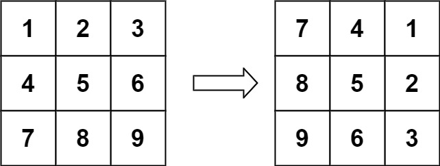
Input: matrix = [[1,2,3],[4,5,6],[7,8,9]] Output: [[7,4,1],[8,5,2],[9,6,3]]
Example 2:
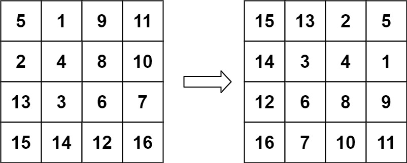
Input: matrix = [[5,1,9,11],[2,4,8,10],[13,3,6,7],[15,14,12,16]] Output: [[15,13,2,5],[14,3,4,1],[12,6,8,9],[16,7,10,11]]
Constraints:
n =matrix.length= matrix[i].length1 <n <= 20=-1000 <matrix[i][j] <= 1000=
※ 2.19.2.1. Constraints and Edge Cases
The important part is that everything has to be in-place.
It seems as though using helper aux buffers might be a gray-area for that.
※ 2.19.2.2. My Solution (Code)
※ 2.19.2.2.1. v0: failed, got confused by the boundaries
this kind of question is all about the boundary management and the off-by-one errors.
1: from collections import deque 2: 3: class Solution: 4: │ def rotate(self, matrix: List[List[int]]) -> None: 5: │ │ """ 6: │ │ Do not return anything, modify matrix in-place instead. 7: │ │ """ 8: │ │ n = len(matrix) 9: │ │ offset = 0 10: │ │ m = n 11: │ │ 12: │ │ while offset < n // 2: 13: │ │ │ # === read edges into buffers === 14: │ │ │ # top_row: 15: │ │ │ top_buffer = deque() 16: │ │ │ for c in range(offset, n - offset): 17: │ │ │ │ top_buffer.append(matrix[offset][c]) 18: │ │ │ │ 19: │ │ │ bottom_buffer = deque() 20: │ │ │ # reverse direction for bottom buffer 21: │ │ │ # NOTE: we ignore the first element in the slice to avoid duplicates (only for the bottom one) 22: │ │ │ for c in range(n - offset - 1, offset, -1): 23: │ │ │ │ # NOTE: the row = n - offset - 1 24: │ │ │ │ bottom_buffer.append(matrix[n - offset - 1][c]) 25: │ │ │ │ 26: │ │ │ right_buffer = deque() 27: │ │ │ for r in range(offset, n - offset): 28: │ │ │ │ # NOTE: the last column is n - offset - 1 29: │ │ │ │ right_buffer.append(matrix[r][n - offset - 1]) 30: │ │ │ │ 31: │ │ │ left_buffer = deque() 32: │ │ │ # NOTE: ignore the last in the slice to prevent the duplicate 33: │ │ │ for r in range(n - offset - 1, offset, -1): 34: │ │ │ │ left_buffer.append(matrix[r][offset]) 35: │ │ │ │ 36: │ │ │ # ====================== now we do thewrites: ================ 37: │ │ │ 38: │ │ │ # write to top using left buffer: 39: │ │ │ for c in range(offset, n - offset): 40: │ │ │ │ matrix[offset][c] = left_buffer.popleft() 41: │ │ │ │ 42: │ │ │ # write to right using top buffer 43: │ │ │ for r in range(offset, n - offset): 44: │ │ │ │ matrix[r][n - offset - 1] = top_buffer.popleft() 45: │ │ │ │ 46: │ │ │ │ 47: │ │ │ # write to bottom using right buffer: 48: │ │ │ for c in range(n - offset - 1, offset, -1): 49: │ │ │ │ matrix[n - offset - 1][c] = right_buffer.popleft() 50: │ │ │ │ 51: │ │ │ │ 52: │ │ │ # write to left using bottom 53: │ │ │ for r in range(n - offset - 1, offset, -1): 54: │ │ │ │ matrix[r][offset] = bottom_buffer.popleft() 55: │ │ │ │ 56: │ │ │ offset += 1
- Correctness:
- Conceptually on track by extracting edges into buffers and writing them into rotated positions.
- However, this approach is overly complex for the problem requirements.
- Major risk of off-by-one errors, duplicates or missed elements due to managing index ranges carefully.
- Uses extra space for buffers, which violates the in-place constraint.
- Summary:
- Works only if carefully debugged, but this is not the recommended approach for in-place rotation.
※ 2.19.2.2.2. v1: guided: 4-way temp store then merge
1: class Solution: 2: │ def rotate(self, matrix: List[List[int]]) -> None: 3: │ │ """ 4: │ │ Do not return anything, modify matrix in-place instead. 5: │ │ """ 6: │ │ n = len(matrix) 7: │ │ for layer in range(n // 2): 8: │ │ │ 9: │ │ │ # define layer boudaries: 10: │ │ │ first = layer 11: │ │ │ last = n - layer - 1 12: │ │ │ 13: │ │ │ # items in the "buffer" 14: │ │ │ for i in range(first, last): 15: │ │ │ │ # we read them all 16: │ │ │ │ offset = i - first 17: │ │ │ │ top = matrix[first][i] 18: │ │ │ │ left = matrix[last - offset][first] 19: │ │ │ │ bottom = matrix[last][last - offset] 20: │ │ │ │ right = matrix[i][last] 21: │ │ │ │ 22: │ │ │ │ # then we write them, the 90degree rotation 23: │ │ │ │ matrix[first][i] = left 24: │ │ │ │ matrix[last - offset][first] = bottom 25: │ │ │ │ matrix[last][last - offset] = right 26: │ │ │ │ matrix[i][last] = top
※ 2.19.2.2.3. v2: minimising the extra temp variables.
We can just store one element then rotate the rest.
1: class Solution: 2: │ def rotate(self, matrix: List[List[int]]) -> None: 3: │ │ """ 4: │ │ Do not return anything, modify matrix in-place instead. 5: │ │ """ 6: │ │ n = len(matrix) 7: │ │ 8: │ │ for layer in range(n // 2): 9: │ │ │ first = layer 10: │ │ │ last = n - 1 - layer 11: │ │ │ 12: │ │ │ for i in range(first, last): 13: │ │ │ │ offset = i - first 14: │ │ │ │ temp = matrix[first][i] # save top 15: │ │ │ │ 16: │ │ │ │ # perform 4-way swap clockwise 17: │ │ │ │ matrix[first][i] = matrix[last - offset][first] # left to top 18: │ │ │ │ matrix[last - offset][first] = matrix[last][last - offset] # bottom to left 19: │ │ │ │ matrix[last][last - offset] = matrix[i][last] # right to bottom 20: │ │ │ │ matrix[i][last] = temp # top to right
※ 2.19.2.2.4. v3: transpose the matrix then reverse the rows:
clear 2-steps here:
1: class Solution: 2: │ def rotate(self, matrix: List[List[int]]) -> None: 3: │ │ n = len(matrix) 4: │ │ # Transpose 5: │ │ for i in range(n): 6: │ │ │ for j in range(i+1, n): 7: │ │ │ │ matrix[i][j], matrix[j][i] = matrix[j][i], matrix[i][j] 8: │ │ │ │ 9: │ │ # Reverse each row 10: │ │ for row in matrix: 11: │ │ │ row.reverse()
※ 2.19.2.3. My Approach/Explanation
See versions above
※ 2.19.2.4. My Learnings/Questions
- I know this kind of matrix manipulations can have a lot of subtle bugs, please help me enumerate them
- Subtle, common bugs:
- Off-by-One Errors:
- When iterating elements for swap within a layer, loop from first to last - 1 (not including last), otherwise repeated swaps or out-of-bound accesses happen.
- Incorrect offset Computation:
- Calculate
offset = i - firstprecisely to map indices correctly.
- Calculate
- Layer Limits:
- Iterate only through
n // 2layers; middle layer in odd-sized matrix remains untouched.
- Iterate only through
- Temp Variable:
- Forgetting to use a temporary variable results in corrupted values due to overwriting.
- Indexing Mistakes:
- Confusing row-column indexing across four parts can cause wrong assignments.
- Not Handling Single-Element Matrix:
- For
n=1, the matrix is unchanged and should be considered.
- For
- Off-by-One Errors:
※ 2.19.2.5. [Optional] Additional Context
<e.g., “I struggled with X”, “I want to know about alternative algorithms”, etc.>
※ 2.19.3. [144] Spiral Matrix (54) redo accuracy_problem pointer_management direction_simulation
Given an m x n matrix, return all elements of the matrix in
spiral order.
Example 1:
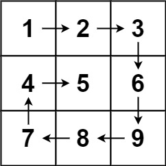
Input: matrix = [[1,2,3],[4,5,6],[7,8,9]] Output: [1,2,3,6,9,8,7,4,5]
Example 2:

Input: matrix = [[1,2,3,4],[5,6,7,8],[9,10,11,12]] Output: [1,2,3,4,8,12,11,10,9,5,6,7]
Constraints:
m =matrix.length=n =matrix[i].length=1 <m, n <= 10=-100 <matrix[i][j] <= 100=
※ 2.19.3.1. Constraints and Edge Cases
<list constraints, input limits, or tricky edge cases here>
※ 2.19.3.2. My Solution (Code)
※ 2.19.3.2.1. v0: failed initial
1: class Solution: 2: │ def spiralOrder(self, matrix: List[List[int]]) -> List[int]: 3: │ │ R, C = len(matrix), len(matrix[0]) 4: │ │ # define boundaries to be constricted: 5: │ │ left, right = 0, C 6: │ │ top, down = 0, R 7: │ │ 8: │ │ ans = [] 9: │ │ 10: │ │ while left < right or top < down: 11: │ │ │ # get the top row from left to right: 12: │ │ │ ans.extend(matrix[top][left:right + 1]) 13: │ │ │ top += 1 14: │ │ │ 15: │ │ │ # get the right column from top to bottom 16: │ │ │ for row in range(top, down + 1): 17: │ │ │ │ ans.append(matrix[row][right]) 18: │ │ │ right -= 1 19: │ │ │ 20: │ │ │ # get the bottom row from 21: │ │ │ ans.extend(reversed(matrix[bottom][left:right + 1])) 22: │ │ │ bottom -= 1 23: │ │ │ 24: │ │ │ # get the left col: 25: │ │ │ for row in range(bottom + 1, top - 1, -1): 26: │ │ │ │ ans.append(matrix[row][left]) 27: │ │ │ left += 1 28: │ │ │ 29: │ │ return ans
You initialize right = C and down = R, which are one past the last valid index since Python uses 0-based indexing.
Valid column indices go from 0 to C-1
Valid row indices go from 0 to R-1
Correct initialization should be:
Show/Hide Python Code1: left, right = 0, C - 1 2: top, down = 0, R - 1
- mixing up of
downandbottomvariables – just silly wrong while loop termination
using
while left < right or top < down:allows the loop to continue even when only one of those holds.
But in a spiral traversal, the bounds should stay consistent, terminating when either rows or columns have been fully covered.
You should use: while left <= right and top <= down:
Off-by-one errors in slices and loops When slicing lists or iterating, inclusive/exclusive boundaries must be handled carefully.
For example, in
matrix[top][left:right + 1], slicing withright + 1is correct if right is the last column index.But your initial right was C, which is out of range.
Similarly, in
for row in range(top, down + 1):, you want to iterate from top row to down row inclusive, so adding +1 is correct if down is the last valid row index.- Issues in your initial v0 version include:
- Misinitialization of right and down as one past the last index:
- right = C, down = R (should be C - 1, R - 1).
- Incorrect loop condition using or:
- while left < right or top < down keeps executing too long.
- Mixing variable names down and bottom.
- Boundary off-by-ones on slices and range limits.
- These lead to out-of-range indexing and repeated items.
- Misinitialization of right and down as one past the last index:
※ 2.19.3.2.2. v1: correct without the accuracy issues
1: from typing import List 2: 3: class Solution: 4: │ def spiralOrder(self, matrix: List[List[int]]) -> List[int]: 5: │ │ if not matrix or not matrix[0]: 6: │ │ │ return [] 7: │ │ │ 8: │ │ rows, cols = len(matrix), len(matrix[0]) 9: │ │ left, right = 0, cols - 1 10: │ │ top, bottom = 0, rows - 1 11: │ │ result = [] 12: │ │ 13: │ │ while left <= right and top <= bottom: 14: │ │ │ # Traverse top row from left to right 15: │ │ │ for col in range(left, right + 1): 16: │ │ │ │ result.append(matrix[top][col]) 17: │ │ │ top += 1 18: │ │ │ 19: │ │ │ # Traverse right column from top to bottom 20: │ │ │ for row in range(top, bottom + 1): 21: │ │ │ │ result.append(matrix[row][right]) 22: │ │ │ right -= 1 23: │ │ │ 24: │ │ │ if top <= bottom: 25: │ │ │ │ # Traverse bottom row from right to left 26: │ │ │ │ for col in range(right, left - 1, -1): 27: │ │ │ │ │ result.append(matrix[bottom][col]) 28: │ │ │ │ bottom -= 1 29: │ │ │ │ 30: │ │ │ if left <= right: 31: │ │ │ │ # Traverse left column from bottom to top 32: │ │ │ │ for row in range(bottom, top - 1, -1): 33: │ │ │ │ │ result.append(matrix[row][left]) 34: │ │ │ │ left += 1 35: │ │ │ │ 36: │ │ return result
※ 2.19.3.2.3. v2: generalised direction simulation:
this will work for irregular matrices and non-square shapes
Tradeoff is \(O(mn)\) extra space for the visited set.
1: def spiralOrder(matrix): 2: │ if not matrix: 3: │ │ return [] 4: │ R, C = len(matrix), len(matrix[0]) 5: │ seen = [[False]*C for _ in range(R)] 6: │ dr = [0,1,0,-1] # directions: right, down, left, up 7: │ dc = [1,0,-1,0] 8: │ r = c = di = 0 9: │ ans = [] 10: │ for _ in range(R*C): 11: │ │ ans.append(matrix[r][c]) 12: │ │ seen[r][c] = True 13: │ │ nr, nc = r + dr[di], c + dc[di] 14: │ │ if 0 <= nr < R and 0 <= nc < C and not seen[nr][nc]: 15: │ │ │ r, c = nr, nc 16: │ │ else: 17: │ │ │ di = (di + 1) % 4 18: │ │ │ r, c = r + dr[di], c + dc[di] 19: │ return ans
※ 2.19.3.3. My Approach/Explanation
It’s just traversal with sound pointer management, but I struggled with the accuracy of it.
※ 2.19.3.4. My Learnings/Questions
- there’s 2 main things to do:
- decide whether you want close-open or close-close slice intervals and stick to it – it affects the rest of the boundary definitions in the loops.
- decide on the while loop end conditions
- Main points for accuracy and pointer management in spiral traversal:
- Consistent use of inclusive vs exclusive boundaries:
- Your boundaries left, right, top, bottom refer to inclusive indices of columns and rows.
- Therefore, when slicing or looping, ranges usually use right + 1 or bottom + 1 as end in Python (range() is exclusive at end).
- Loop termination condition:
- It should be while left <= right and top <= bottom: — both row and column intervals must be valid.
- After each directional traversal, update corresponding boundary:
- After top row → top += 1
- After right column → right -= 1
- After bottom row → bottom -= 1
- After left column → left += 1
- Always check if rows/columns remain before traversing bottom and left edges:
- This prevents duplicates or index errors if the spiral closes in asymmetrically.
- Avoid off-by-one errors:
- Carefully verify range() parameters and whether you want inclusive or exclusive indexing.
- Avoid variable name confusion:
- Use a single consistent name for each boundary (e.g., bottom instead of mixing down and bottom).
- Consistent use of inclusive vs exclusive boundaries:
※ 2.19.3.5. [Optional] Additional Context
I’m oddly struggling with the accuracy management of this pointer boundary stuff.
※ 2.19.4. [145] Set Matrix Zeroes (73) in_place_markers
Given an m x n integer matrix matrix, if an element is 0, set its
entire row and column to 0’s.
You must do it in place.
Example 1:
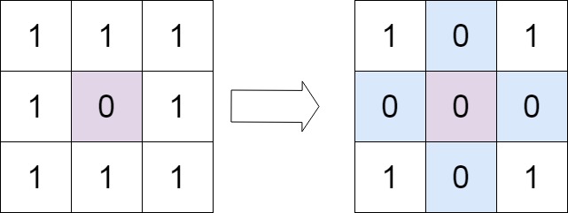
Input: matrix = [[1,1,1],[1,0,1],[1,1,1]] Output: [[1,0,1],[0,0,0],[1,0,1]]
Example 2:
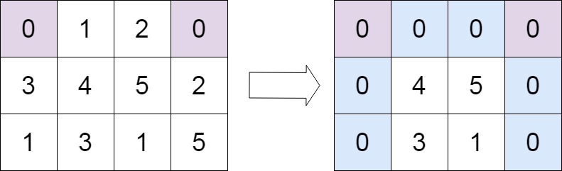
Input: matrix = [[0,1,2,0],[3,4,5,2],[1,3,1,5]] Output: [[0,0,0,0],[0,4,5,0],[0,3,1,0]]
Constraints:
m =matrix.length=n =matrix[0].length=1 <m, n <= 200=-2=^{=31}= <= matrix[i][j] <= 2=31= - 1=
Follow up:
- A straightforward solution using
O(mn)space is probably a bad idea. - A simple improvement uses
O(m + n)space, but still not the best solution. - Could you devise a constant space solution?
※ 2.19.4.1. Constraints and Edge Cases
Nothingness much.
※ 2.19.4.2. My Solution (Code)
※ 2.19.4.2.1. v0: correct, slow, just does a traversal
1: class Solution: 2: │ def setZeroes(self, matrix: List[List[int]]) -> None: 3: │ │ """ 4: │ │ Do not return anything, modify matrix in-place instead. 5: │ │ """ 6: │ │ R, C = len(matrix), len(matrix[0]) 7: │ │ 8: │ │ for r, c in [(r, c) for r in range(R) for c in range(C) if matrix[r][c] == 0]: 9: │ │ │ # zero the row: 10: │ │ │ for col in range(C): 11: │ │ │ │ matrix[r][col] = 0 12: │ │ │ │ 13: │ │ │ for row in range(R): 14: │ │ │ │ matrix[row][c] = 0
- Complexity analysis:
time Finding zero positions:
O(R * C)For each zero found (suppose k zeros), zeroing row and column takes
O(R + C).Worst case: if all elements are zero, complexity is \(O(R * C * (R + C)) \approx O(n^3)\) for square matrix \(n * n\).
space The list to store positions of zeros takes \(O(k)\) space, up to \(O(R*C)\) in worst case.
No extra matrices.
※ 2.19.4.2.2. v1: 3-pass sets, space and time optimisation by preventing excess operations
Collect all the targets once
1: 2: class Solution: 3: │ def setZeroes(self, matrix: List[List[int]]) -> None: 4: │ │ R, C = len(matrix), len(matrix[0]) 5: │ │ rows, cols = set(), set() 6: │ │ 7: │ │ # First pass: find zero rows and columns 8: │ │ for r in range(R): 9: │ │ │ for c in range(C): 10: │ │ │ │ if matrix[r][c] == 0: 11: │ │ │ │ │ rows.add(r) 12: │ │ │ │ │ cols.add(c) 13: │ │ │ │ │ 14: │ │ # Second pass: zero rows 15: │ │ for r in rows: 16: │ │ │ for c in range(C): 17: │ │ │ │ matrix[r][c] = 0 18: │ │ │ │ 19: │ │ # Third pass: zero columns 20: │ │ for c in cols: 21: │ │ │ for r in range(R): 22: │ │ │ │ matrix[r][c] = 0 23:
※ 2.19.4.2.3. v2: Optimal in-place markers
We can use the first row and first column’s zeroes as markers
1: class Solution: 2: │ def setZeroes(self, matrix: List[List[int]]) -> None: 3: │ │ R, C = len(matrix), len(matrix[0]) 4: │ │ 5: │ │ first_row_zero = any(matrix[0][c] == 0 for c in range(C)) 6: │ │ first_col_zero = any(matrix[r][0] == 0 for r in range(R)) 7: │ │ 8: │ │ # Use first row and column as markers 9: │ │ for r in range(1, R): 10: │ │ │ for c in range(1, C): 11: │ │ │ │ if matrix[r][c] == 0: 12: │ │ │ │ │ matrix[r][0] = 0 13: │ │ │ │ │ matrix[0][c] = 0 14: │ │ │ │ │ 15: │ │ # Zero rows based on first column 16: │ │ for r in range(1, R): 17: │ │ │ if matrix[r][0] == 0: 18: │ │ │ │ for c in range(1, C): 19: │ │ │ │ │ matrix[r][c] = 0 20: │ │ │ │ │ 21: │ │ # Zero columns based on first row 22: │ │ for c in range(1, C): 23: │ │ │ if matrix[0][c] == 0: 24: │ │ │ │ for r in range(1, R): 25: │ │ │ │ │ matrix[r][c] = 0 26: │ │ │ │ │ 27: │ │ # Zero first row if needed 28: │ │ if first_row_zero: 29: │ │ │ for c in range(C): 30: │ │ │ │ matrix[0][c] = 0 31: │ │ │ │ 32: │ │ # Zero first column if needed 33: │ │ if first_col_zero: 34: │ │ │ for r in range(R): 35: │ │ │ │ matrix[r][0] = 0
※ 2.19.4.3. My Approach/Explanation
I’m just doing a naive approach
※ 2.19.4.4. My Learnings/Questions
the optimal solution is pretty nifty. It’s not hard to get to this realisation actually.
TRICK: we can use in-place markers for grids / matrices
I learnt that if I use a generator, then because it’s lazily taken, it can get affected by my main loops where I’m doing the looping. Quite a fun realisation.
Using a listcomp will snapshot it correctly.
Using a generator (which is lazy) can give us false-positives.
※ 2.19.4.5. [Optional] Additional Context
I’m pretty fast with the naive approach.
※ 2.19.5. [146] Happy Number (202) tortoise_hare_method integer_division_vs_float_division test_for_loop
Write an algorithm to determine if a number n is happy.
A happy number is a number defined by the following process:
- Starting with any positive integer, replace the number by the sum of the squares of its digits.
- Repeat the process until the number equals 1 (where it will stay), or it loops endlessly in a cycle which does not include 1.
- Those numbers for which this process ends in 1 are happy.
Return true if n is a happy number, and false if not.
Example 1:
Input: n = 19 Output: true Explanation: 12 + 92 = 82 82 + 22 = 68 62 + 82 = 100 12 + 02 + 02 = 1
Example 2:
Input: n = 2 Output: false
Constraints:
1 <n <= 2=31= - 1=
※ 2.19.5.1. Constraints and Edge Cases
Nothing fancy here
※ 2.19.5.2. My Solution (Code)
※ 2.19.5.2.1. v0: my solution, cycle detection using sets
1: class Solution: 2: │ def isHappy(self, n: int) -> bool: 3: │ │ visited = set() 4: │ │ 5: │ │ while n != 1: 6: │ │ │ copy = n 7: │ │ │ next_n = 0 8: │ │ │ while copy > 0: 9: │ │ │ │ next_n += (copy % 10) ** 2 10: │ │ │ │ # GOTCHA: this has to be an integer division, not a float division. This was a source of error 11: │ │ │ │ copy //= 10 12: │ │ │ │ 13: │ │ │ if next_n in visited: # we have found a loop: 14: │ │ │ │ return False 15: │ │ │ │ 16: │ │ │ visited.add(next_n) 17: │ │ │ n = next_n 18: │ │ │ 19: │ │ return True
- Time and Space Complexity
- Time Complexity:
- Each number mapped to the next number tends to decrease or go into a cycle quickly. Since the sum of squares of digits reduces large numbers eventually, the maximum number to consider is bounded.
- Roughly, time complexity is \(O(log n)\) (digits of n) times a small constant number of iterations before cycle detection, so overall close to \(O(log n)\).
- Space Complexity:
- Using a set to store visited numbers may store up to \(O(log n)\) numbers (worst case). This is efficient for the input constraints.
- Time Complexity:
※ 2.19.5.2.2. v1: Floyd’s Tortoise and Hare cycle detection (better for space saving)
This is actually pretty cute.
1: class Solution: 2: │ def isHappy(self, n: int) -> bool: 3: │ │ def next_num(num): 4: │ │ │ return sum(int(s) ** 2 for s in str(num)) 5: │ │ │ 6: │ │ slow = n 7: │ │ fast = next_num(n) 8: │ │ 9: │ │ while fast != 1 and slow != fast: 10: │ │ │ slow = next_num(slow) 11: │ │ │ fast = next_num(next_num(fast)) 12: │ │ │ 13: │ │ return fast == 1
Another approach uses Floyd’s Cycle Detection (Tortoise and Hare algorithm) to detect cycles without extra space:
- Uses two pointers moving at different speeds on sequence of numbers.
- If they meet (enter cycle), return False; if slow pointer reaches 1 → return True.
- Uses \(O(1)\) additional space.
※ 2.19.5.3. My Approach/Explanation
The idea is that we are iterating through different values of “n”.
If it’s something we have seen before, then we have found a loop and things are going to be infinite.
※ 2.19.5.4. My Learnings/Questions
- we can get next num using string conversions:
sum(int(digit) ** 2 for digit in str(num)) - Careful not to accidentally do float divisions
GOTCHA: we need to do the digit stripping using integer divison and not float division.
this is right: copy //= 10
this is wrong: copy /= 10
※ 2.19.6. [147] Plus One (66) carry_propagation in_place
You are given a large integer represented as an integer array
digits, where each digits[i] is the i=^{=th} digit of the integer.
The digits are ordered from most significant to least significant in
left-to-right order. The large integer does not contain any leading
0’s.
Increment the large integer by one and return the resulting array of digits.
Example 1:
Input: digits = [1,2,3] Output: [1,2,4] Explanation: The array represents the integer 123. Incrementing by one gives 123 + 1 = 124. Thus, the result should be [1,2,4].
Example 2:
Input: digits = [4,3,2,1] Output: [4,3,2,2] Explanation: The array represents the integer 4321. Incrementing by one gives 4321 + 1 = 4322. Thus, the result should be [4,3,2,2].
Example 3:
Input: digits = [9] Output: [1,0] Explanation: The array represents the integer 9. Incrementing by one gives 9 + 1 = 10. Thus, the result should be [1,0].
Constraints:
1 <digits.length <= 100=0 <digits[i] <= 9=digitsdoes not contain any leading0’s.
※ 2.19.6.1. Constraints and Edge Cases
nothing much here
※ 2.19.6.2. My Solution (Code)
※ 2.19.6.2.1. v1: my solution (aux list)
1: class Solution: 2: │ def plusOne(self, digits: List[int]) -> List[int]: 3: │ │ carry = 1 4: │ │ ans = [] 5: │ │ 6: │ │ for idx in range(len(digits) - 1, -1, -1): 7: │ │ │ new_digit = digits[idx] + carry 8: │ │ │ 9: │ │ │ if new_digit >= 10: 10: │ │ │ │ # GOTCHA: this was my initial fault 11: │ │ │ │ # new_digit, carry = divmod(new_digit, 10) 12: │ │ │ │ carry, new_digit = divmod(new_digit, 10) 13: │ │ │ else: 14: │ │ │ │ carry = 0 15: │ │ │ │ 16: │ │ │ ans.append(new_digit) 17: │ │ │ 18: │ │ # remember to clear out pending carry! 19: │ │ if carry: 20: │ │ │ ans.append(carry) 21: │ │ │ 22: │ │ return list(reversed(ans))
※ 2.19.6.2.2. v2: in-place solution
1: class Solution: 2: │ def plusOne(self, digits: List[int]) -> List[int]: 3: │ │ n = len(digits) 4: │ │ 5: │ │ for i in range(n-1, -1, -1): 6: │ │ │ digits[i] += 1 7: │ │ │ if digits[i] < 10: 8: │ │ │ │ return digits 9: │ │ │ digits[i] = 0 10: │ │ │ 11: │ │ # If we reach here, it means all digits were `9` 12: │ │ return [1] + digits
- Efficient and clear.
- Stops processing as soon as no carry is needed.
- Handles leading carry by prepending 1.
※ 2.19.6.3. My Approach/Explanation
- this is the human way of doing addition, we’re just doing it in reverse then reversing the result
※ 2.19.6.4. My Learnings/Questions
- Small Python idiom for reversing:
ans[::-1]is more idiomatic thanlist(reversed(ans))but both are fine. - GOTCHA: my
divmodis sometimes wrong. Some things to note:the unpacking is based on the name, we get
divthen themodso if we do
div, mod = divmod(251, 10)thendiv = 25,mod = 1- in this case, the carry value is actually the div, the remaining is the remainder, that’s why we set it like so.
※ 2.19.6.5. [Optional] Additional Context
Confidence booster!!!
※ 2.19.7. [148] Pow(x, n) (50) redo fast_exponentiation binary_exponentiation classic
Implement pow(x,
n), which calculates x raised to the power n (i.e., x=^{=n}).
Example 1:
Input: x = 2.00000, n = 10 Output: 1024.00000
Example 2:
Input: x = 2.10000, n = 3 Output: 9.26100
Example 3:
Input: x = 2.00000, n = -2 Output: 0.25000 Explanation: 2-2 = 1/22 = 1/4 = 0.25
Constraints:
-100.0 < x < 100.0-2=^{=31}= <= n <= 2=31=-1=nis an integer.- Either
xis not zero orn > 0. -10=^{=4}= <= x=n= <= 10=4
※ 2.19.7.1. Constraints and Edge Cases
<list constraints, input limits, or tricky edge cases here>
※ 2.19.7.2. My Solution (Code)
※ 2.19.7.2.1. v0: cheat using python syntax
1: class Solution: 2: │ def myPow(self, x: float, n: int) -> float: 3: │ │ return x ** n
※ 2.19.7.2.2. v1: fast exponentiation, binary exponentiation
Fast exponentiation, also called binary exponentiation or exponentiation by squaring, is a method to compute \[x^n\] using only about \[O(\log n)\] multiplications instead of \[O(n)\].
1: class Solution: 2: │ def myPow(self, x: float, n: int) -> float: 3: │ │ if n == 0: 4: │ │ │ return 1.0 5: │ │ if n < 0: 6: │ │ │ return 1 / self.myPow(x, -n) 7: │ │ half = self.myPow(x, n // 2) 8: │ │ if n % 2 == 0: 9: │ │ │ return half * half 10: │ │ else: 11: │ │ │ return half * half * x
another way to write this:
1: class Solution: 2: │ def myPow(self, x: float, n: int) -> float: 3: │ │ # iterative fast exponentiation: 4: │ │ N = n # N is the running exponent that we shall be using 5: │ │ 6: │ │ if N < 0: # if negative exponent, then make it positive, use the reiprocal for the operand 7: │ │ │ x = 1 / x 8: │ │ │ N = -N 9: │ │ │ 10: │ │ result = 1.0 11: │ │ curr_product = x 12: │ │ 13: │ │ while N > 0: 14: │ │ │ # if first bit is 1 / it's odd: 15: │ │ │ if N % 2 == 1: 16: │ │ │ │ result *= curr_product # decrement so that it's even and we can power this 17: │ │ │ │ 18: │ │ │ curr_product *= curr_product 19: │ │ │ N //= 2 # half the exponent 20: │ │ │ 21: │ │ return result
- Approach:
- Initialize result = 1, current power = base \[x\], exponent = \[n\]
- Loop while exponent > 0:
- If current exponent bit is 1, multiply result by current power
- Square current power
- Shift exponent right by 1 bit (divide by 2)
- Return result
※ 2.19.7.3. My Approach/Explanation
I’ve a feeling this is just about 2s complement encoding form
My other idea was to just find nearest power of 2, then do the bitshifting as needed.
then for the remaining indices, manually multiply it.
※ 2.19.7.4. My Learnings/Questions
intuition behind fast exponentiation: The key insight is to use the binary representation of the exponent \[n\] and properties of exponents:
- \[x^{a+b} = x^a \times x^b\]
- \[x^{2b} = (x^b)^2\]
So instead of multiplying \[x\] by itself \[n\] times, you:
- Express \[n\] in binary.
- Decompose \[x^n\] into a product of powers of \[x\] with exponents as powers of two.
- Compute these powers by repeatedly squaring \[x\].
- Multiply the necessary powers corresponding to 1-bits in the binary representation of \[n\].
- benefits of using fast exponentiation:
- Runs in \[O(\log n)\] time, drastically faster than naive \[O(n)\].
- Uses repeated squaring to reuse intermediate results efficiently.
- Fits well with binary computers, exploiting bit manipulation.
※ 2.19.7.5. [Optional] Additional Context
quite wild that I somehow had the intuition for binary exponentiation at the back of my mind somewhere.
※ 2.19.8. [149] ⭐️ Multiply Strings (43) multiplication_algo
Given two non-negative integers num1 and num2 represented as
strings, return the product of num1 and num2, also represented as a
string.
Note: You must not use any built-in BigInteger library or convert the inputs to integer directly.
Example 1:
Input: num1 = "2", num2 = "3" Output: "6"
Example 2:
Input: num1 = "123", num2 = "456" Output: "56088"
Constraints:
1 <num1.length, num2.length <= 200=num1andnum2consist of digits only.- Both
num1andnum2do not contain any leading zero, except the number0itself.
※ 2.19.8.1. Constraints and Edge Cases
- rmb to strip leading zeroes
- rmb to early return if one of the inputs is 0
※ 2.19.8.2. My Solution (Code)
※ 2.19.8.2.1. guided optimal
1: class Solution: 2: │ def multiply(self, num1: str, num2: str) -> str: 3: │ │ # early returns if either of them is 0 4: │ │ if num1 == "0" or num2 == "0": 5: │ │ │ return "0" 6: │ │ │ 7: │ │ n, m = len(num1), len(num2) 8: │ │ max_num_places = n + m 9: │ │ result = [0] * max_num_places 10: │ │ 11: │ │ # We process from least significant digit to most significant digit 12: │ │ for i in range(n-1, -1, -1): 13: │ │ │ for j in range(m-1, -1, -1): 14: │ │ │ │ unit_idx = i + j + 1 15: │ │ │ │ carry_idx = i + j 16: │ │ │ │ 17: │ │ │ │ mul = int(num1[i]) * int(num2[j]) 18: │ │ │ │ partial_sum = mul + result[i + j + 1] 19: │ │ │ │ 20: │ │ │ │ unit_digit = partial_sum % 10 21: │ │ │ │ carry_value = partial_sum // 10 22: │ │ │ │ 23: │ │ │ │ result[unit_idx] = unit_digit 24: │ │ │ │ result[carry_idx] += carry_value 25: │ │ │ │ 26: │ │ # Convert result to string skipping leading zeros 27: │ │ result_str = [] 28: │ │ leading_zero = True 29: │ │ for digit in result: 30: │ │ │ 31: │ │ │ leading_zero = leading_zero and digit == 0 32: │ │ │ # skip leading zeroes 33: │ │ │ if leading_zero: 34: │ │ │ │ continue 35: │ │ │ │ 36: │ │ │ result_str.append(str(digit)) 37: │ │ │ 38: │ │ return "".join(result_str) if result_str else "0"
Explanation of how this works
The result array stores intermediate sums.
We multiply digit by digit starting from least significant digits (i, j) from right to left.
The product is added to result[i+j+1] because digits in multiplication “line up” along positions with sum of indices.
Carry is pushed to result[i+j].
After computation, leading zeros are trimmed in the final answer.
※ 2.19.8.3. My Approach/Explanation
This is the multiplication algo, just that my brain is fried and I can’t figure it out at the moment.
Will have to redo this question.
※ 2.19.8.4. My Learnings/Questions
Core Intuition: For two digits at positions
i(from right in num1) andj(from right in num2), the product contributes to positioni + j + 1in the result array (starting from 0 on the left, with leftmost digit being the most significant).Any overflow (carry) is propagated to
i + j, the next more significant position.
Describing the multiplication algo from school
The multiplication of two numbers digit by digit involves multiplying each digit of one number by each digit of the other, shifting the result by the corresponding place (like in school).
Some useful observations:
- the intermediate sums can be stored in a total of (n + m) places
- the usual method is always from least significant to most significant digit
- we know that for each sub-multiplication, we get a partial sum. \(\implies\) where to keep that partial sum?
- the results array itself
- so when we get partial sum for
(i , j), we should store it atresult[i + j + 1]. This is the observation that digits in multiplication “line up” along positions with sum of indices. - the carry value should be pushed to
result[i + j], which is one to the left of idx =[i + j + 1]
- remember the trivial situations :
- if at least one of them is “0” then can early return
- there may be trailing 0s in the result, we will have to trim them.
※ 2.19.9. [150] Detect Squares (2013) cartesian_plane
You are given a stream of points on the X-Y plane. Design an algorithm that:
- Adds new points from the stream into a data structure. Duplicate points are allowed and should be treated as different points.
- Given a query point, counts the number of ways to choose three points from the data structure such that the three points and the query point form an axis-aligned square with positive area.
An axis-aligned square is a square whose edges are all the same length and are either parallel or perpendicular to the x-axis and y-axis.
Implement the DetectSquares class:
DetectSquares()Initializes the object with an empty data structure.void add(int[] point)Adds a new pointpoint = [x, y]to the data structure.int count(int[] point)Counts the number of ways to form axis-aligned squares with pointpoint = [x, y]as described above.
Example 1:
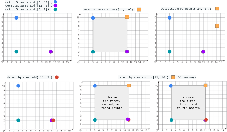
Input
["DetectSquares", "add", "add", "add", "count", "count", "add", "count"]
[[], [[3, 10]], [[11, 2]], [[3, 2]], [[11, 10]], [[14, 8]], [[11, 2]], [[11, 10]]]
Output
[null, null, null, null, 1, 0, null, 2]
Explanation
DetectSquares detectSquares = new DetectSquares();
detectSquares.add([3, 10]);
detectSquares.add([11, 2]);
detectSquares.add([3, 2]);
detectSquares.count([11, 10]); // return 1. You can choose:
// - The first, second, and third points
detectSquares.count([14, 8]); // return 0. The query point cannot form a square with any points in the data structure.
detectSquares.add([11, 2]); // Adding duplicate points is allowed.
detectSquares.count([11, 10]); // return 2. You can choose:
// - The first, second, and third points
// - The first, third, and fourth points
Constraints:
point.length =2=0 <x, y <= 1000=- At most
3000calls in total will be made toaddandcount.
※ 2.19.9.1. Constraints and Edge Cases
<list constraints, input limits, or tricky edge cases here>
※ 2.19.9.2. My Solution (Code)
※ 2.19.9.2.1. v0 failed to comprehend the multiplicity property
this will not work because “duplicate points are allowed and should be treated as different points”.
1: from collections import defaultdict 2: class DetectSquares: 3: │ 4: │ def __init__(self): 5: │ │ # an x value -> a list of corresponding points on that line 6: │ │ self.x_aligned = defaultdict(list) 7: │ │ self.y_aligned = defaultdict(list) 8: │ │ self.points = set() 9: │ │ 10: │ def add(self, point: List[int]) -> None: 11: │ │ x, y = point 12: │ │ self.points.add((x, y)) 13: │ │ self.x_aligned[x].append((x, y)) 14: │ │ self.y_aligned[y].append((x, y)) 15: │ │ 16: │ def count(self, point: List[int]) -> int: 17: │ │ t_x, t_y = point 18: │ │ candidates_x = self.x_aligned[t_x] 19: │ │ candidates_y = self.y_aligned[t_y] 20: │ │ 21: │ │ if not candidates_x or not candidates_y: 22: │ │ │ return 0 23: │ │ │ 24: │ │ distances_x = [(y - t_y, x, y) for x, y for candidates_x] 25: │ │ distances_y = [(x - t_x, x, y) for x, y for candidates_y] 26: │ │ 27: │ │ 28: │ │ 29: │ │ 30: │ │ 31: # Your DetectSquares object will be instantiated and called as such: 32: # obj = DetectSquares() 33: # obj.add(point) 34: # param_2 = obj.count(point)
Core mistake: not directly finding the missing corners
Given a query point (x, y), to find all axis-aligned squares with sides parallel to axes, you need to find another point on the same row or column at an equal non-zero distance from (x, y) in both x and y directions, and then check if the other two corners exist.
- multiplicity requirement not handled
- if we use a set for the points, we lose that
- a point can be added more than once \(\implies\) we need to use a dict to do a frequency count
- key property to count squares: we need to find a pair of points: (x2, y) an (x, y2) for a query point (x, y) such that they’re of the same distance.
※ 2.19.9.2.2. v1: guided solution
1: from collections import defaultdict 2: class DetectSquares: 3: │ 4: │ def __init__(self): 5: │ │ self.points = defaultdict(int) 6: │ │ 7: │ def add(self, point: List[int]) -> None: 8: │ │ self.points[tuple(point)] += 1 9: │ │ 10: │ def count(self, point: List[int]) -> int: 11: │ │ x, y = point 12: │ │ result = 0 13: │ │ 14: │ │ # get for same x: 15: │ │ for (can_x, can_y), count in list(self.points.items()): 16: │ │ │ # reject impossibles 17: │ │ │ if not (can_x == x and can_y != y): 18: │ │ │ │ continue 19: │ │ │ │ 20: │ │ │ side = abs(can_y - y) 21: │ │ │ # possibility 1: we check to the right: 22: │ │ │ p1 = (x, can_y) 23: │ │ │ p2 = (x + side, y) 24: │ │ │ p3 = (x + side, can_y) 25: │ │ │ num_p1, num_p2, num_p3 = [self.points[pt] for pt in [p1, p2, p3]] 26: │ │ │ result += (num_p1 * num_p2 * num_p3) 27: │ │ │ 28: │ │ │ # possibility 2: we check to the left: 29: │ │ │ p4 = (x - side, can_y) 30: │ │ │ p5 = (x - side, y) 31: │ │ │ num_p4, num_p5 = [self.points[pt] for pt in [p4, p5]] 32: │ │ │ result += (num_p1 * num_p4 * num_p5) 33: │ │ │ 34: │ │ return result
※ 2.19.9.3. My Approach/Explanation
My solution was too convoluted again.
Here’s one way to write this
1: from collections import defaultdict 2: class DetectSquares: 3: │ 4: │ def __init__(self): 5: │ │ self.points = defaultdict(int) 6: │ │ 7: │ def add(self, point: List[int]) -> None: 8: │ │ self.points[tuple(point)] += 1 9: │ │ 10: │ def count(self, point: List[int]) -> int: 11: │ │ x, y = point 12: │ │ result = 0 13: │ │ 14: │ │ # get for same x: 15: │ │ for (can_x, can_y), count in list(self.points.items()): 16: │ │ │ # reject impossibles 17: │ │ │ if not (can_x == x and can_y != y): 18: │ │ │ │ continue 19: │ │ │ │ 20: │ │ │ side = abs(can_y - y) 21: │ │ │ # possibility 1: we check to the right: 22: │ │ │ p1 = (x, can_y) 23: │ │ │ p2 = (x + side, y) 24: │ │ │ p3 = (x + side, can_y) 25: │ │ │ num_p1, num_p2, num_p3 = [self.points[pt] for pt in [p1, p2, p3]] 26: │ │ │ result += (num_p1 * num_p2 * num_p3) 27: │ │ │ 28: │ │ │ # possibility 2: we check to the left: 29: │ │ │ p4 = (x - side, can_y) 30: │ │ │ p5 = (x - side, y) 31: │ │ │ num_p4, num_p5 = [self.points[pt] for pt in [p4, p5]] 32: │ │ │ result += (num_p1 * num_p4 * num_p5) 33: │ │ │ 34: │ │ return result
and this is a further cleanup:
1: from collections import defaultdict 2: class DetectSquares: 3: │ 4: │ def __init__(self): 5: │ │ self.point_count = defaultdict(int) 6: │ │ 7: │ def add(self, point: List[int]) -> None: 8: │ │ self.point_count[tuple(point)] += 1 9: │ │ 10: │ def count(self, point: List[int]) -> int: 11: │ │ x, y = point 12: │ │ result = 0 13: │ │ # Scan all points that share the same x 14: │ │ for (cx, cy), cnt in self.point_count.items(): 15: │ │ │ # candidate should share x, but not y 16: │ │ │ if cx == x and cy != y: 17: │ │ │ │ side = abs(cy - y) 18: │ │ │ │ # check to the right 19: │ │ │ │ p1 = (x, cy) 20: │ │ │ │ p2 = (x + side, y) 21: │ │ │ │ p3 = (x + side, cy) 22: │ │ │ │ result += (self.point_count[p1] * 23: │ │ │ │ │ │ │ self.point_count[p2] * 24: │ │ │ │ │ │ │ self.point_count[p3]) 25: │ │ │ │ # check to the left 26: │ │ │ │ p4 = (x - side, y) 27: │ │ │ │ p5 = (x - side, cy) 28: │ │ │ │ result += (self.point_count[p1] * 29: │ │ │ │ │ │ │ self.point_count[p4] * 30: │ │ │ │ │ │ │ self.point_count[p5]) 31: │ │ return result
※ 2.19.9.4. My Learnings/Questions
Have to try keep things simple by looking at the most complex function first.
some things that make it simple for us to find the other 3 points:
- fix an axis first, in this case we fix the x axis.
- then find 2 other points that make sense for every candidate in this axis.
※ 2.19.9.5. [Optional] Additional Context
And with this we’re done!!
※ 2.19.10. [exposure-1] Alice and Bob Playing Flower Game (3021) counting
Alice and Bob are playing a turn-based game on a field, with two lanes
of flowers between them. There are x flowers in the first lane between
Alice and Bob, and y flowers in the second lane between them.
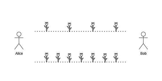
The game proceeds as follows:
- Alice takes the first turn.
- In each turn, a player must choose either one of the lane and pick one flower from that side.
- At the end of the turn, if there are no flowers left at all, the current player captures their opponent and wins the game.
Given two integers, n and m, the task is to compute the number of
possible pairs (x, y) that satisfy the conditions:
- Alice must win the game according to the described rules.
- The number of flowers
xin the first lane must be in the range[1,n]. - The number of flowers
yin the second lane must be in the range[1,m].
Return the number of possible pairs (x, y) that satisfy the
conditions mentioned in the statement.
Example 1:
Input: n = 3, m = 2 Output: 3 Explanation: The following pairs satisfy conditions described in the statement: (1,2), (3,2), (2,1).
Example 2:
Input: n = 1, m = 1 Output: 0 Explanation: No pairs satisfy the conditions described in the statement.
Constraints:
1 <n, m <= 10=5
※ 2.19.10.1. Constraints and Edge Cases
- nothing fancy here
※ 2.19.10.2. My Solution (Code)
※ 2.19.10.2.1. v0: optimal counting solution
1: class Solution: 2: │ def flowerGame(self, n: int, m: int) -> int: 3: │ │ """ 4: │ │ The objective is for alice to win, she also starts first ==> x, y form an odd pair 5: │ │ 6: │ │ I know that it's also a build-up of values, because we 7: │ │ 8: │ │ question boils down to: given n and m, 9: │ │ pick odd pairs (x, y) such that x in [1, n] and y in [1, m] 10: │ │ 11: │ │ so (x + y) must be odd 12: │ │ 13: │ │ This is just a pure combinations question. 14: │ │ case 1: x is odd, y is even 15: │ │ case 2: y is odd, x is even 16: │ │ """ 17: │ │ get_odd_nums = lambda num: (num + 1) // 2 18: │ │ get_even_nums = lambda num: (num) // 2 19: │ │ case_1 = get_odd_nums(n) * get_even_nums(m) 20: │ │ case_2 = get_even_nums(n) * get_odd_nums(m) 21: │ │ 22: │ │ return case_1 + case_2
※ 2.19.10.3. My Approach/Explanation
initially felt like some DP thing but after understanding the question, it ended up being just a combinations question.
※ 2.19.10.4. My Learnings/Questions
- have patience, reading the preamble for longer ones should be done patiently because misinterpreting it == total and complete failure
- Data structure-based approaches (e.g., DP): Not needed, as there’s no substate dependency—everything boils down to parity, which is stateless.
- Intuition: Since the only property that matters is the parity (\(x+y\) odd), count all pairs with one odd and one even, using arithmetic tricks to get those counts instantly.
※ 2.19.10.5. [Optional] Additional Context
This was satisfying. Just writing out the understanding was sufficient to reduce the problem to one of counting. Initially, it felt like some DP accumulation kind of problem, then it became clearer that it’s just combinatorial.
The time management part, questions like this seems to have a longer time just comprehending things, but it’s alright. As long as I’m focused on the question, the time I take is pretty short.
※ 2.19.11. [exposure-2] Sort Matrix by Diagonals (3446)
You are given an n x n square matrix of integers grid. Return the
matrix such that:
- The diagonals in the bottom-left triangle (including the middle diagonal) are sorted in non-increasing order.
- The diagonals in the top-right triangle are sorted in non-decreasing order.
Example 1:
Input: grid = [[1,7,3],[9,8,2],[4,5,6]]
Output: [[8,2,3],[9,6,7],[4,5,1]]
Explanation:
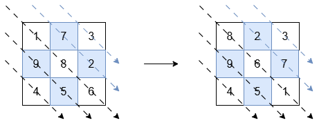
The diagonals with a black arrow (bottom-left triangle) should be sorted in non-increasing order:
[1, 8, 6]becomes[8, 6, 1].[9, 5]and[4]remain unchanged.
The diagonals with a blue arrow (top-right triangle) should be sorted in non-decreasing order:
[7, 2]becomes[2, 7].[3]remains unchanged.
Example 2:
Input: grid = [[0,1],[1,2]]
Output: [[2,1],[1,0]]
Explanation:
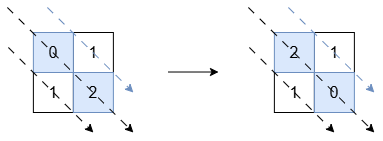
The diagonals with a black arrow must be non-increasing, so [0, 2] is
changed to [2, 0]. The other diagonals are already in the correct
order.
Example 3:
Input: grid = [BROKEN LINK: 1]
Output: [BROKEN LINK: 1]
Explanation:
Diagonals with exactly one element are already in order, so no changes are needed.
Constraints:
grid.length =grid[i].length= n1 <n <= 10=-10=^{=5}= <= grid[i][j] <= 10=5
※ 2.19.11.1. Constraints and Edge Cases
- just for n <= 1, can early return
※ 2.19.11.2. My Solution (Code)
※ 2.19.11.2.1. v0: correct, passes all diagonals traversal
1: class Solution: 2: │ def sortMatrix(self, grid: List[List[int]]) -> List[List[int]]: 3: │ │ """ 4: │ │ It's about uniquely identifying diagonals, then doing sorting within it. 5: │ │ 6: │ │ looks like a linear approach might work based on the input sizes 7: │ │ 8: │ │ uniquely identifying a diagonal: using the "y intercepts": row - col 9: │ │ """ 10: │ │ n = len(grid) 11: │ │ if n <= 1: 12: │ │ │ return grid 13: │ │ │ 14: │ │ for diagonal in range(-(n - 1), n): # NOTE: valid diagonals are from -(n - 1) to +(n - 1) inclusive 15: │ │ │ # diagonal 16: │ │ │ is_reverse = diagonal < 0 17: │ │ │ sort_candidates = [] # (val) 18: │ │ │ for row in range(0, n): 19: │ │ │ │ if 0 <= (col:=(row - diagonal)) < n: 20: │ │ │ │ │ sort_candidates.append(grid[row][col]) 21: │ │ │ │ │ 22: │ │ │ sorted_candidates = sorted(sort_candidates, reverse=(is_reverse)) 23: │ │ │ for row in range(0, n): 24: │ │ │ │ if 0 <= (col:=(row - diagonal)) < n: 25: │ │ │ │ │ grid[row][col] = sorted_candidates.pop() 26: │ │ │ │ │ 27: │ │ return grid
This runs in \(O(n^{2}\log n)\) time.
※ 2.19.11.2.2. v1: optimal bucketing method
1: from typing import List 2: from collections import defaultdict 3: 4: class Solution: 5: │ def sortMatrix(self, grid: List[List[int]]) -> List[List[int]]: 6: │ │ n = len(grid) 7: │ │ diags = defaultdict(list) 8: │ │ # Collect elements by diagonal index 9: │ │ for r in range(n): 10: │ │ │ for c in range(n): 11: │ │ │ │ diags[r - c].append(grid[r][c]) 12: │ │ # Sort each group by correct rule 13: │ │ for d in diags: 14: │ │ │ if d >= 0: 15: │ │ │ │ diags[d].sort(reverse=True) # bottom-left, non-increasing 16: │ │ │ else: 17: │ │ │ │ diags[d].sort(reverse=False) # top-right, non-decreasing 18: │ │ # Place sorted back into grid 19: │ │ for r in range(n): 20: │ │ │ for c in range(n): 21: │ │ │ │ grid[r][c] = diags[r - c].pop(0) 22: │ │ return grid
It’s not asymptotically better, in fact space use is in \(O(n)\)
※ 2.19.11.3. My Approach/Explanation
This is just a traversal of matrix diagonals
※ 2.19.11.4. My Learnings/Questions
- Careful: since we are doing pops we need to sort in the opposite order. So bottom half is supposed to be non-increasing: so we sort in increasing and pop it and get things in non-increasing order. Mirrored argument for the top right half.
※ 2.19.12. [exposure-3] Walking Robot Simulation (874) simulation turtlebot
A robot on an infinite XY-plane starts at point (0, 0) facing north.
The robot receives an array of integers commands, which represents a
sequence of moves that it needs to execute. There are only three
possible types of instructions the robot can receive:
-2: Turn left90degrees.-1: Turn right90degrees.1 <k <= 9=: Move forwardkunits, one unit at a time.
Some of the grid squares are obstacles. The i=^{=th} obstacle is at
grid point obstacles[i] = (x=_{=i}=, y=i=)=. If the robot runs
into an obstacle, it will stay in its current location (on the block
adjacent to the obstacle) and move onto the next command.
Return the maximum squared Euclidean distance that the robot reaches
at any point in its path (i.e. if the distance is 5, return 25).
Note:
- There can be an obstacle at
(0, 0). If this happens, the robot will ignore the obstacle until it has moved off the origin. However, it will be unable to return to(0, 0)due to the obstacle. - North means +Y direction.
- East means +X direction.
- South means -Y direction.
- West means -X direction.
Example 1:
Input: commands = [4,-1,3], obstacles = []
Output: 25
Explanation:
The robot starts at (0, 0):
- Move north 4 units to
(0, 4). - Turn right.
- Move east 3 units to
(3, 4).
The furthest point the robot ever gets from the origin is (3, 4),
which squared is 3=^{=2}= + 4=2= = 25= units away.
Example 2:
Input: commands = [4,-1,4,-2,4], obstacles = [BROKEN LINK: 2,4]
Output: 65
Explanation:
The robot starts at (0, 0):
- Move north 4 units to
(0, 4). - Turn right.
- Move east 1 unit and get blocked by the obstacle at
(2, 4), robot is at(1, 4). - Turn left.
- Move north 4 units to
(1, 8).
The furthest point the robot ever gets from the origin is (1, 8),
which squared is 1=^{=2}= + 8=2= = 65= units away.
Example 3:
Input: commands = [6,-1,-1,6], obstacles = [BROKEN LINK: 0,0]
Output: 36
Explanation:
The robot starts at (0, 0):
- Move north 6 units to
(0, 6). - Turn right.
- Turn right.
- Move south 5 units and get blocked by the obstacle at
(0,0), robot is at(0, 1).
The furthest point the robot ever gets from the origin is (0, 6),
which squared is 6=^{=2}= = 36= units away.
Constraints:
1 <commands.length <= 10=4commands[i]is either-2,-1, or an integer in the range[1, 9].0 <obstacles.length <= 10=4-3 * 10=^{=4}= <= x=i=, y=i= <= 3 * 10=4- The answer is guaranteed to be less than
2=^{=31}.
※ 2.19.12.1. Constraints and Edge Cases
Straightforward grid simulation, this is actually turtlebot classic interview question.
※ 2.19.12.2. My Solution (Code)
※ 2.19.12.2.1. v0: my version good enough
1: class Solution: 2: │ def robotSim(self, commands: List[int], obstacles: List[List[int]]) -> int: 3: │ │ """ 4: │ │ Robot, what to simulate? 5: │ │ 1. current facing direction, we can use bearings for this 0 (north), 90 (east), 180 (south), 270 (west) and so on 6: │ │ 2. current location this is just cartesian, represents the CELL it's currenly at (r, c) 7: │ │ 8: │ │ We start at origin, don't need to do an obstacle check. 9: │ │ 10: │ │ Preproc the obstacles as a set of coordinates. 11: │ │ 12: │ │ We parse command. 13: │ │ """ 14: │ │ obstacles = {tuple(coord) for coord in obstacles} 15: │ │ curr_location = (0, 0) 16: │ │ curr_direction = 0 17: │ │ 18: │ │ def get_next_cell(curr_cell, direction): 19: │ │ │ match direction: 20: │ │ │ │ case 0: # move north 21: │ │ │ │ │ return (curr_cell[0], curr_cell[1] + 1) 22: │ │ │ │ case 90: # East 23: │ │ │ │ │ return (curr_cell[0] + 1, curr_cell[1]) 24: │ │ │ │ case 180: # South 25: │ │ │ │ │ return (curr_cell[0], curr_cell[1] - 1) 26: │ │ │ │ case 270: # West 27: │ │ │ │ │ return (curr_cell[0] - 1, curr_cell[1]) 28: │ │ │ │ │ 29: │ │ max_dist = 0 30: │ │ 31: │ │ for c_idx, command in enumerate(commands): 32: │ │ │ # print(f"[Command {c_idx}]: {command} @ {curr_location} facing {curr_direction}") 33: │ │ │ match command: 34: │ │ │ │ case -2: # turning command, turn left 90 35: │ │ │ │ │ if curr_direction == 0: 36: │ │ │ │ │ │ curr_direction = 270 37: │ │ │ │ │ else: 38: │ │ │ │ │ │ curr_direction -= 90 39: │ │ │ │ │ │ 40: │ │ │ │ case -1: # turning command, turn right 90 41: │ │ │ │ │ if curr_direction == 270: 42: │ │ │ │ │ │ curr_direction = 0 43: │ │ │ │ │ else: 44: │ │ │ │ │ │ curr_direction += 90 45: │ │ │ │ │ │ 46: │ │ │ │ case k if 1 <= k <= 9: # movement command 47: │ │ │ │ │ for step_idx in range(k): 48: │ │ │ │ │ │ next_cell = get_next_cell(curr_location, curr_direction) 49: │ │ │ │ │ │ if next_cell in obstacles: 50: │ │ │ │ │ │ │ break 51: │ │ │ │ │ │ │ 52: │ │ │ │ │ │ curr_location = next_cell 53: │ │ │ │ │ │ 54: │ │ │ │ │ dist = (curr_location[0] ** 2) + (curr_location[1]**2) 55: │ │ │ │ │ # print(f"\tmoved to [{curr_location}] dist = {dist}, best_dist = {max_dist}") 56: │ │ │ │ │ max_dist = max(max_dist, dist) 57: │ │ │ │ │ 58: │ │ return max_dist
complexity
Time Complexity:
\(O(N+M)\), where N is the number of commands and M is the number of obstacles. Each move command can result in up to 9 steps (since 1≤k≤9), but overall work is linear in command count, as each movement checks at most one obstacle per step.
Space Complexity: \(O(M)\), storing every obstacle as a tuple in a set for fast lookup.
- Improvement suggestions:
Modulo arithmetic for rotation:
Instead of cumbersome if/else for left/right, use:
Show/Hide Python- Codecurr_direction = (curr_direction - 90) nil 360 # left curr_direction = (curr_direction + 90) nil 360 # right
Direction lookup:
Replace match/case for movement with a direction map or list:
Show/Hide Python Codedirection_map = {0: (0,1), 90:(1,0), 180:(0,-1), 270:(-1,0)} dx, dy = direction_map[curr_direction]
Cleaner step loop:
Unify movement logic and maximize clarity by using list/dict for directions instead of angle values if preferred.
Remove unused/debug variables for clarity and brevity.
※ 2.19.12.2.2. v1: bot version: use direction vector
1: class Solution: 2: │ def robotSim(self, commands: List[int], obstacles: List[List[int]]) -> int: 3: │ │ OBSTACLES = set(map(tuple, obstacles)) 4: │ │ DIRS = [(0, 1), (1, 0), (0, -1), (-1, 0)] # N, E, S, W 5: │ │ x = y = dir_idx = 0 6: │ │ max_dist = 0 7: │ │ 8: │ │ for cmd in commands: 9: │ │ │ if cmd == -2: # turn left 10: │ │ │ │ dir_idx = (dir_idx - 1) % 4 11: │ │ │ elif cmd == -1: # turn right 12: │ │ │ │ dir_idx = (dir_idx + 1) % 4 13: │ │ │ else: 14: │ │ │ │ dx, dy = DIRS[dir_idx] 15: │ │ │ │ for _ in range(cmd): 16: │ │ │ │ │ nx, ny = x + dx, y + dy 17: │ │ │ │ │ if (nx, ny) in OBSTACLES: 18: │ │ │ │ │ │ break 19: │ │ │ │ │ x, y = nx, ny 20: │ │ │ │ │ max_dist = max(max_dist, x*x + y*y) 21: │ │ return max_dist
The use of direction deltas will be useful for representing NESW and we can use the relative positioning of the direction idx to just have a pointer to that direction. That’s what dir_idx is doing above and using the modulo 4.
I agree that this is simple to reason with.
※ 2.19.12.3. My Approach/Explanation
my version simulated direction using bearing angle, the bot tells me to just use unit vectors.
※ 2.19.12.4. My Learnings/Questions
- We have 2 options to represent directions here. My approach was to use bearing angles, and the suggested approach is to just use unit vectors and the relative index of the vectors can be used to keep track of the current direction. I think that works well.
<what did you learn? any uncertainties or questions?>
※ 3. Depth Gains
※ 3.1. Context
※ 3.1.1. Objectives:
After the initial breadth phase, I have a rough idea of my weaknesses and strengths.
The two concrete objectives to achieve:
- personal topical weaknesses + general revision
- general topical weaknesses
The long-term gains this needs to give:
- easier memory hacking (just need to go thru on my website and I will retain this)
- topical confidence and exposure
- consolidated sections within my notes, not just verbose ones.
※ 3.1.2. Process:
So, I’ll just be doing this for each concrete objective:
Skim through topical questions from my responses to 150, topic by topic in reverse chronological order, focus on the questions that have unusually long times (attempt + review).
For each just essayplan it: make an attempt to recall, then just rewrite the answer / copy paste it into leetcode as a solution (for only 40% of the questions) asap.
The objective here is just plain memory hacking.
This will contribute to the pattern recognition + boilerplate aspects too.
For the general categories,
Read the labuladong parts, enque the extra, similar questions that have been suggested within it, this is visible even if it’s a locked article. Just cover all the patterns that labuladong goes through. This will give the depth in areas that are traditionally harder.
Also cover the classic algos that neetcode goes through.
Alternate doing and essayplanning, change ratio based on tiredness (more tired, just stick to essayplanning).
※ 3.1.3. Resourcing:
Time: I’m now writing this strategy on .
I have set D-Day as
For the first iteration of this depth phase, I want to allocate 3 days, 18h each (with 80% productive time gives roughly 14h in a day and 4h cummulative on breaks.)
This means - will go to Depth phase.
I will re-evaluate after that, or try a v0 of exposure phase before coming back to depth phase.
Some references:
For personal weaknesses, it’s this document.
For global weaknesses,
- labuladong has got other locked articles that I should look into as well.
- leetcode has topic-specific problem lists
- e.g. DP problems
- neetcode has a simple dive into the different specific algos that appear. These look like a good first-pass, there are some linked questions there that can be attempted.
※ 3.2. Priority Queues
※ 3.2.1. Topical PQ
Given Bucket A (needs revision + blind) vs Bucket B (review-only now; handle breadth/exposure later),
| Priority | Topic | Bucket | Canonical question types | Med/Hard didactic LC (historical) to review | Med/Hard LC (BLIND) to attempt |
|---|---|---|---|---|---|
| 1 | DP – Knapsack family (0/1, unbounded, bounded; order-of-loops; 1-D rollup; comb vs perm) | A | 0/1 knapsack; unbounded; subset/partition; coin change; 2-D knapsack | ✅🤔 322 Change (M), ✅🤔 518 Coin Change II (M), ✅🤔 416 Partition Equal Subset Sum (M), ✅🤔 494 Target Sum (M), 🤔 474 Ones and Zeroes (M) | 😈 2218 Max Value of K Coins From Piles (H), ✅⚠️😈 956 Tallest Billboard (H), 🤔 1049 Last Stone Weight II (M) |
| 2 | DP – State machine & Interval & Regex | A | Stock DP (cooldown/fees/K-transactions); interval DP; regex/wildcard | ✅🤔 309 Best Time w/ Cooldown (M), 😈 188 Best Time IV (H), 🤔 123 Best Time III (M/H), ✅😈 312 Burst Balloons (H), ✅😈 10 RegEx Matching (H) | 😈 1547 Min Cost to Cut a Stick (H), 🤔 714 Best Time w/ Fee (M), 🤔 375 Guess Number II (M) |
| 3 | String DP / subsequences | A | Edit distance; LCS/SCS; distinct subsequences; interleaving; palindromic subseq | ✅🤔 72 Edit Distance (M), ✅😈 115 Distinct Subsequences (H-ish), ✅🤔 1143 LCS (M), ✅🤔 97 Interleaving String (M), 🤔 1312 Min Insertions to Palindrome (M) | 😈 1092 Shortest Common Supersequence (H), 🤔 712 Min ASCII Delete Sum (M), 🤔 1035 Uncrossed Lines (M) |
| 4 | Sliding window / Two pointers | A | Fixed/variable window; frequency maps; at-most/exact-K distinct; expand/contract | ✅🤔 3 Longest Substring w/o Repeat (M), ✅😈 76 Minimum Window Substring (H), ✅🤔 424 Longest Repeating Char Replacement (M), ✅🤔 438 Find All Anagrams (M) | 😈 992 Subarrays with K Different Integers (H), ✅🤔 1234 Replace Substring for Balanced String (M), ✅🤔 1456 Max Vowels in Substring (M) |
| 5 | Graph: Topological + BFS shortest path + lexicographic | A | Kahn vs DFS topo; indegree nuances; BFS on word graphs; lexicographic topo/paths | ✅🤔 210 Course Schedule II (M), ✅😈 332 Reconstruct Itinerary (H), ✅🤔 127 Word Ladder (M/H) | ✅😈 126 Word Ladder II (H), ✅😈 269 Alien Dictionary (H), ✅😈 1203 Sort Items by Groups & Deps (H) |
| 6 | Union-Find + MST | A | DSU with path compression + rank; cycle detection; components; Kruskal MST | ✅🤔 684 Redundant Connection (M), 🤔 547 Number of Provinces (M), 🤔 1319 Make Network Connected (M), 🤔 1584 Min Cost to Connect Points (M) | 😈 685 Redundant Connection II (H), 😈 952 Largest Component by Common Factor (H), 🤔 990 Satisfiability of Equality Equations (M) |
| 7 | Greedy & Intervals | A | Sort-by-end; activity selection; interval partitioning; weighted scheduling; exchange arguments | 🤔 56 Merge Intervals (M), 🤔 435 Non-overlapping Intervals (M), 🤔 452 Min Arrows to Burst Balloons (M), 🤔 763 Partition Labels (M), 😈 135 Candy (H) | 😈 871 Min Refuel Stops (H), 😈 1235 Job Scheduling (H), 🤔 621 Task Scheduler (M), 😈 630 Course Schedule III (H) |
| 8 | Binary search on answer | A | Feasibility check + monotone predicate; capacity/speed/sum limits | ✅🤔 875 Koko Eating Bananas (M), ✅🤔 1011 Ship Packages (M), 😈 410 Split Array Largest Sum (H) | 🤔 1482 Min Days to Make Bouquets (M), 🤔 1552 Magnetic Force Between Two Balls (M), 🤔 1802 Max Value at Given Index (M) |
| 9 | Monotonic stack / queue | A | Next greater; decreasing stacks for range; histogram/rectangle; monotonic queue | ✅🤔 739 Daily Temperatures (M), ✅😈 42 Trapping Rain Water (H), ✅😈 84 Largest Rectangle in Histogram (H), ✅😈 239 Sliding Window Maximum (H) | 😈 85 Maximal Rectangle (H), ✅🤔 316 Remove Duplicate Letters (M), ✅⚠️🤔 456 132 Pattern (M) |
| 10 | Heaps / k-way merge / streaming | A | k-way merge; selection; streaming medians; top-K; scheduling with PQ | 😈 23 Merge k Sorted Lists (H), 🤔 347 Top K Frequent Elements (M), 😈 295 Median from Data Stream (H) | 😈 480 Sliding Window Median (H), 🤔 373 Find K Pairs with Smallest Sums (M), 🤔 692 Top K Frequent Words (M) |
| 11 | Dijkstra / shortest-path variants | B | Weighted shortest paths; constraints (stops/time); max-probability | 🤔 743 Network Delay Time (M), 🤔 787 Cheapest Flights K Stops (M/H), 🤔 1631 Path With Min Effort (M), 🤔 1514 Path with Max Probability (M) | (Defer to exposure) |
| 12 | Prefix sums / hashing | B | Subarray sums; prefix-mod; 2D prefix | 🤔 560 Subarray Sum = K (M), 🤔 974 Subarray Sums Divisible by K (M), 🤔 523 Continuous Subarray Sum (M), 🤔 1248 Nice Subarrays (M) | (Defer to exposure) |
| 13 | Trees (classic) | B | LCA; max path; build/serialize; DFS aggregations | 🤔 236 LCA (M), 😈 124 Binary Tree Max Path Sum (H), 😈 297 Serialize/Deserialize (H), 🤔 105 Build Tree (M) | (Defer to exposure) |
| 14 | Tries / prefix trees | B | Insert/search; wildcard; dictionary ops | 🤔 208 Implement Trie (M), 🤔 211 Add & Search Word (M) | (Defer to exposure) |
| 15 | Backtracking (you’ve advanced here) | B | Sudoku; N-Queens; Word Search; partitions | 😈 37 Sudoku Solver (H), 😈 51 N-Queens (H), 🤔 79 Word Search (M), 🤔 131 Palindrome Partitioning (M) | (Defer to exposure) |
| 16 | Bit manipulation / math | B | XOR families; bit DP tricks | 🤔 201 Bitwise AND of Range (M), 🤔 137 Single Number II (M), 🤔 260 Single Number III (M) | (Defer to exposure) |
Notes on tailoring to your retros & HRT bar
I put Knapsack DP at number 1 because your Day 3 notes flag this as the most stubborn gap (loop direction, 1-D rollup, comb vs perm).* State-machine DP + Interval DP stay top-tier because they appear in your slow list and are classic “hard DP” signals at elite firms. Sliding window remains A because `76` was slow for you; it’s a high-leverage skill that often shows up as “fast but careful”. Topological/lexicographic graph and Union-Find are A due to your template weaknesses (Kahn’s direction; DSU optimizations). Dijkstra/weighted paths are B for depth (time sink) but are covered during Exposure, after you’ve locked the above.
※ 3.2.2. Hard Questions PQ
Some guidelines about doing hards (from this thread).
Here’s an exerpt:
Here's a detailed response to your two tasks — combining expert strategies for tackling Leetcode hard questions and a close analysis of your progress logs with practical next steps. *** ## 1. Expert Strategies for Cracking Leetcode Hard Questions ### a. Systematic Approach to Hard Problems - **Problem Simplification**: Break down the "story" or "fluff" in the prompt and distill every problem into: *inputs*, *transform/process*, *desired outputs*. Rephrase the question in your own words before coding — this makes edge cases and hidden constraints explicit.[1][2] - **Input Size = Solution Constraints**: The input constraints *explicitly* signal feasible algorithms: │ - *Small inputs (n≤20, 30)*: Backtracking, brute-force, or all-subsets approaches will work. │ - *Medium inputs (n≤1,000)*: Typically allows O(n²) or O(n²log n) dynamic programming or graph solutions. │ - *Large inputs (n≥10⁴–10⁵)*: Forces you to think in O(nlog n) or O(n), often with greedy, prefix/suffix, or data structure optimization.[2][3] - **Pattern Recognition**: Most hards are nontrivial combinations of *medium-level patterns* (see: DP, topological sort, sliding window, union find, etc.).[4] - **Brute Force to Insight**: Start with a naïve (but correct) approach. A slow, brute-force version is your analytical base; try to optimize from there. Often, this will reveal subproblem overlap, optimal substructure, or a feasible direction for pruning. - **Edge Cases and Walkthroughs**: For every new algorithmic thought, *walk through* it on sample and edge cases in detail. - **Debugging and Failing Faster**: It's normal to get stuck on hards; the goal is to *generate hypotheses*, test, and fail quickly. Interpret wrong outputs as steps toward correct logic.[1] - **Reading Solutions with Purpose**: After honest attempts, *read solution explanations for patterns used and why brute force failed* instead of just copying code. This builds long-term pattern recognition. ### b. Psychological Tactics — Mindset for Hards - **Normalize Failure**: Top coders and interviewers consistently emphasize: *the goal in a hard is not always to solve it*, but to demonstrate process, hypotheses, and adaptation under pressure.[5][6] - **Growth over Ego**: Avoid conflating inability to do a hard with lack of intelligence. Most hard Leetcode problems are not meant to be solved from scratch under time pressure, even by top engineers.[7][5] - **Measure Progress Correctly**: Many world-class interviewees report initially failing most hards and only solving them after repeated practice and conscious pattern-building.[8][7] ### c. Specific Tactics for Leetcode Hards - **Categorize by Pattern**: Keep a running list of which canonical patterns you see in hards (e.g., "DP on states + clever graph", "difference-based DP", "indexed counting" etc.). - **Input-Driven Filtering**: Before you even begin writing code: │ 1. Glance at the input size ranges and deduce time complexity needed. │ 2. List possible classes of algorithms that fit those constraints. - **Look for Hidden Reductions**: Many hards can be cracked by *reducing* or transforming the problem into a classic (graph/DP/set) base. - **Templates for Classes of Problems**: Prepare templates for "difference-based DP" (Tallest Billboard), "multi-source BFS" (Word Ladder II), "two-phase topological sort" (Sort Items by Groups), etc. - **Mental Model for Hards**: Treat the first 15min as *exploration*: mapping edge cases, feasible brute force, possible state representations, and recognizing dead ends as part of the process. *** ## 2. Commentary on Your Progress Log & Strategy ### Progress Log & Recent Strategy Tweaks You write: > These blinds are absolutely devastating my confidence. > > What I realise is that doing hards should probably not be my current priority. My current priority should be to cover the canonical forms so that the limiting factor is NOT the fundamentals. > > ...I do realise that Hards are "just" a mix of multiple concepts. It's extra HARD when I'm attempting them without the knowledge that I need. This is slowing me down... I will try to do more blind mediums and probably not many hards (or a token hard just to get humbled). I also realise that the partitioning problems are something I need a little more coverage on. **Analysis & Advice:** - **Excellent Self-Diagnosis:** │ You're absolutely correct: Most "hard" Leetcode problems are two or more canonical ideas intertwined with a non-obvious reduction or state representation. Seen in your logs: Word Break II (backtracking + memoization), Tallest Billboard (difference DP), Sort Items by Groups (multi-level topo sort). - **Right Call: Prioritize Canonical Patterns.** │ You're exactly where strong candidates should be: realizing hards mean almost nothing if the med-level "atoms" aren't automated first. Efficient mastery of these patterns lets you *compose* solutions to hards. - **Build Up, Don't Burn Out.** │ The psychic toll of failing hards without feedback is real and well-known. Your plan to re-emphasize medium-level canonical practice, spacing exposure to hards, is aligned with the highest-yield learning research (and what top coders recommend).[9][10][5][7][8] - **Confident Fundamentals = Hard Solutions.** │ Your reflections match expert advice: depth in fundamentals leads to hards feeling more like challenging *puzzles* than insurmountable walls. You'll soon find that a "new hard" is really “Wow, it’s just a twist on difference-based DP and subset sum.” - **Keep Up the Logging.** │ Your logs are full of in-the-moment reasoning and strategic retrospectives — this is the sort of *active reflection* that accelerates mastery and makes bottlenecks clear. │ *** ## Actionable Next Steps - **Continue to Master Mediums:** │ For each topic in your priority list, do both revisits and "blinds" to prove automation and identify gaps in pattern recall. - **For Hards:** │ 1. **Scaffold Hard Problems:** Before doing a full blind, rewrite the classic medium versions. Only then attempt the hard — this primes your mind for the typical reductions/compositions. │ 2. **After timeout/failure:** Instead of spending time brute-forcing, *immediately* seek a top-rated community writeup and extract the *reasoning arc* (not just the trick). Add these to your notes. │ 3. **Occasional “Humbling” Token Hard:** Keeps you in check and familiarizes you with real interview conditions, but maintain majority focus on pattern automation. - **Template Tracker:** │ Build a summary "cheatsheet" for the key templates you see in both mediums and hards. - **Input Size Triaging:** │ Make it a ritual: list possible algorithmic classes based on input constraints before writing any detailed plan. - **Mindset:** │ Remind yourself that failing hards — especially under strict time and blind conditions — is normal and expected, even among elite coders. Progress is in pattern comprehension and recall speed, not problem-solve rate on hards. │ *** ## Bottom Line - You're experiencing the *normal*, optimal pain of leveling up in algorithmic problem solving. - Your calibration is dead on: meditate and re-automate canonical patterns, build intuition for how hards combine them, and gradually increase "hard" exposure as you master more "atomic" skills. - Continue reading and summarizing explanations for unsolved hards — crib their state reductions and pattern merges into your own log. You are *exactly* on track — stay the course, and keep using reflection and targeted practice to close those last gaps. [1] https://www.youtube.com/watch?v=OTNe0eV8418 [2] https://www.designgurus.io/answers/detail/how-to-solve-leetcode-problems-as-a-beginner [3] https://www.designgurus.io/answers/detail/what-are-the-strategies-for-solving-np-hard-problems-in-interviews [4] https://blog.algomaster.io/p/15-leetcode-patterns [5] https://www.youtube.com/watch?v=TsVzk5jyHyc [6] https://www.reddit.com/r/leetcode/comments/wsehjv/how_to_solve_hard_problems/ [7] https://leetcode.com/discuss/career/368612/Folks-who-cracked-google-what-of-LC-hard-problems-were-you-able-to-solve-on-your-own [8] https://code.likeagirl.io/why-500-leetcode-problems-changed-my-life-3b4d5b366508 [9] https://www.reddit.com/r/learnprogramming/comments/ybmrb3/is_leetcode_hard_or_am_i_an_idiot/ [10] https://www.reddit.com/r/cscareerquestions/comments/sgktuv/the_definitive_way_on_how_to_leetcode_properly/ [11] https://ppl-ai-file-upload.s3.amazonaws.com/web/direct-files/attachments/27578138/1cdd58eb-7145-4de6-993d-88513b875d55/paste.txt [12] https://www.youtube.com/watch?v=U0y5UM_WCDg [13] https://www.youtube.com/watch?v=roanIWKtGMY [14] https://leetcode.com/discuss/career/450215/How-to-use-LeetCode-to-help-yourself-efficiently-and-effectively-(for-beginners) [15] https://www.youtube.com/watch?v=snwKjTQlIe4 [16] https://leetcode.com/explore/interview/card/top-interview-questions-hard/ [17] https://news.ycombinator.com/item?id=29804607 [18] https://www.youtube.com/watch?v=aHZW7TuY_yo
※ 3.2.3. Resources
here are some canonical problems:
Show/Hide Md CodeHere’s a structured, **priority queue of canonical computational problems**—ordered by the types that are most frequently found hard in Leetcode interviews. This incorporates both academic canons (like NP-complete problems) and the patterns most cited in industry interviews and Leetcode question statistics. The classification draws from Leetcode tags, Wikipedia computational problem categories, and interview frequency lists. ## Canonical Leetcode Problem Types (from Hardest to Most Classic) | Priority | Problem Type / Canonical Problem | Typical Category | Examples / Comments | |----------|----------------------------------------|-------------------------------|---------------------------------------------------------| | 1 | Advanced Dynamic Programming | NP-Complete, DP | Knapsack, N-Queens, Coin Change, Subset Sum, LIS[5] | | 2 | Advanced Graph Theory and Networks | NP-Complete, Graph | Traveling Salesman, Max-flow/Min-cut, Word Ladder[3] | | 3 | Backtracking / Search + Pruning | NP-Complete, Combinatorial | Sudoku Solver, Permutations, Word Search | | 4 | Combinatorial Optimization, Enumeration| Enumerative, Combinatorics | Partition Problem, Kth Largest Subset | | 5 | Advanced Data Structures | Theoretical/Practical | LRU Cache, Median of Two Sorted Arrays, Interval Merge | | 6 | Scanline, Greedy, and Range Queries | Polynomial Time, Algo Pattern | Trapping Rain Water, Skyline Problem, Interval Covering | | 7 | Medium-level Dynamic Programming | Weakly NP-Complete | Longest Palindromic Substring, Edit Distance | | 8 | Multi-Dimensional DP/Variants | Multidimensional DP | 2D LIS, DP on Trees, Domino Tiling | | 9 | Recursion + Memoization Hybrids | Recursive, DP Mix | Decode Ways, Frog Jump | | 10 | BFS/DFS (Boilerplate) | Graph Traversal | Number of Islands, Course Schedule, Connected Components| | 11 | Classic Sliding Window/Two Pointers | Algorithmic Pattern | Longest Substring Without Repeating Chars | ### Additional Observations - Many “hard” Leetcode problems are cleverly disguised variants or multidimensional/constraint-heavy versions of patterns above—e.g., K-Sum, multidimensional stacking, range queries with additional rules.[2] - Certain problems, like the Knapsack or LIS (Longest Increasing Subsequence), are canonical DP exemplars and regularly cited as patterns to “master”. - LRU Cache, Median of Two Sorted Arrays, and Trapping Rain Water represent canonical tests of algorithmic and data structure ingenuity that come up repeatedly in top company interview lists.[3] ### Where to Find: - Wikipedia categories for reference: │ - [NP-complete problems](https://en.wikipedia.org/wiki/Category:NP-complete_problems) │ - [Weakly NP-complete problems](https://en.wikipedia.org/wiki/Category:Weakly_NP-complete_problems) │ - [Polynomial-time problems](https://en.wikipedia.org/wiki/Category:Polynomial-time_problems) │ - [Enumerative combinatorics](https://en.wikipedia.org/wiki/Enumerative_combinatorics) - Leetcode collects such canonical problems under "hard" filters and in company question frequency lists.[3] ### Suggestion for Exposure - **Focus more** on advanced DP, graph theory, and combinatorics at first—these form the hardest and most canonical problem sets. - For rapid pattern recognition, master LRU Cache, intervals/merge, and sliding window techniques across multiple question variants.[5][3] - Refer to company-specific problem lists for applied, industry-priority filtering.[3] This gives you both the canon and the industry/practice-based prioritization for Leetcode prep.[2][5][3] [1] https://arxiv.org/html/2504.14655v1 [2] https://www.reddit.com/r/leetcode/comments/1aj2oom/mediums_vs_hards/ [3] https://github.com/hxu296/leetcode-company-wise-problems-2022 [4] https://arxiv.org/html/2502.15770v1 [5] https://www.educative.io/blog/coding-interview-leetcode-patterns [6] https://www.youtube.com/watch?v=snwKjTQlIe4 [7] https://news.ycombinator.com/item?id=31450713 [8] https://www.youtube.com/watch?v=-rLAg4kTw9w
- wikipedia has category lists of problems for computational problems:
- NP-compplete problems
- weakly NP-complete problems: contains things like the knapsack problem, partition problem, subset problem
- polynomial time problems
- combinatorics:
※ 3.3. Day 1 Log
First day of depth-focused improvements. I aim to cover all the graph related topics today, from trees to backtracking to graphs. I expect this to take the whole day.
Template weaknesses:
- the kahn’s algo need to know the source and destination for the indegree vs the adj
union find with path suppression and rank tracking optimisations i’m not too good at it yet. Should do one or two union find questions as well.
Show/Hide Python Code1: │class UnionFind: 2: │ │def __init__(self, n: int): 3: │ │ │# Initially, each node is its own parent and its rank (size) is 1 4: │ │ │self.parent = [i for i in range(n)] 5: │ │ │self.rank = [1] * n # can also track size instead of rank 6: │ │ │ 7: │ │def find(self, x: int) -> int: 8: │ │ │""" 9: │ │ │Find the root of x with path compression. 10: │ │ │""" 11: │ │ │if self.parent[x] != x: 12: │ │ │ │# Path compression: set parent[x] directly to the root 13: │ │ │ │self.parent[x] = self.find(self.parent[x]) 14: │ │ │return self.parent[x] 15: │ │ │ 16: │ │def union(self, x: int, y: int) -> bool: 17: │ │ │""" 18: │ │ │Union the sets containing x and y. 19: │ │ │Returns True if merged, False if already in the same set. 20: │ │ │""" 21: │ │ │rootX = self.find(x) 22: │ │ │rootY = self.find(y) 23: │ │ │ 24: │ │ │if rootX == rootY: 25: │ │ │ │return False # already connected 26: │ │ │ │ 27: │ │ │# Union by rank (attach smaller tree to bigger tree) 28: │ │ │if self.rank[rootX] < self.rank[rootY]: 29: │ │ │ │self.parent[rootX] = rootY 30: │ │ │elif self.rank[rootX] > self.rank[rootY]: 31: │ │ │ │self.parent[rootY] = rootX 32: │ │ │else: 33: │ │ │ │self.parent[rootY] = rootX 34: │ │ │ │self.rank[rootX] += 1 35: │ │ │ │ 36: │ │ │return True 37:
Strategy tweaks:
the initial brian dump on reading everything is a little too time taking and it drained me. Especially for the graphs stuff which was PLENTY.
Therefore, here on out, I’ll just look at the code then essay plan the question I’ve already done.
The stars should be rewritten, the TODOs / REDOs also can be done again.
And the TODOs definitely need to be redone.
Tasklist [0/4]:
- Read existing notes on trees, graphs and backtracking
- cover untouched classic graph fundamentals e.g bipartite graphs
[ ]Cover existing questions that I’ve done:- [x] [x] graphs
[X]advanced graphs[ ]backtracking[ ]trees
[ ]Find more canonical problems for these topics- Did find union find problems
Retro:
Going through the already done questions is just linking things in memory. It helps me to do essay plans and articulate better what the broad steps are like.
For the hard questions, I end up seeing a bigger picture to incremental view. I think it’s helping but NOT as much as doing new questions.
I spilled over today but it’s not because of slow workrate. The reading phase has to be better chunked and I should directly review the previous attempts BEFORE reading things on other sites and such.
What I didn’t do well enough was to use the previous timetracking to direct my attention.
I think here’s what I’ll do:
- the ones that I have timetracking which was SLOWER, I’ll ONLY essay plan it. The ones that are faster, I’ll rewrite it for confidence boosts.
- I still feel pretty good. I’m doing alright on time so far.
Tomorrow:
I expect to carry on with the backtracking (stretch goal is tree-stuff) first. I hope to be done way before lunch so that I can do some reading on the DP stuff before lunch.
I’m doing good. Tomorrow I think I’ll be able to cover the rest.
※ 3.3.1. BotGuided: Study Plan Integration and Analysis
Alright — I’ve read through everything you’ve given me, cross-referenced your Day 1 log, your timing data, and your clarified sleep/wake schedule. Here’s the updated, integrated plan and analysis.
※ 3.3.1.1. Part 1: Depth Sprint Targets Overall (20 Questions Priority Queue)
This list is chosen from:
- The slowest timings in Tackling the Basics: Neocode 150 and relevant Basic Grid 83 entries.
- Interview leverage (frequency in FAANG/interview prep lists).
Cases where your notes mention “redo,” “TODO,” or “canonical.”
Ranked Priority List
(★ = high interview leverage, ⏳ = very slow in your logs, ⚠ = marked redo/TODO in notes)
- House Robber I (198) ★⏳
- Decode Ways (91) ★⏳⚠
- Maximum Product Subarray (152) ★⏳⚠
- Edit Distance (72) ★⏳
- Regular Expression Matching (10) ★⚠
- Coin Change (322) ★
- Burst Balloons (312) ★⚠
- Word Ladder II (126) ★⏳
- Reconstruct Itinerary (332) ★⏳
- Minimum Window Substring (76) ★⏳
- Distinct Subsequences (115) ★⏳
- Interleaving String (97) ★⚠
- Longest Increasing Path in a Matrix (329) ★⏳
- Target Sum (494) ★
- Longest Palindromic Substring (5) ⏳
- Bipartite Graph Check ★
- Union-Find Cycle Detection in Graph ★
- Course Schedule II (210) ★⏳
- Word Search II (212) ★⏳
- Partition Equal Subset Sum (416) ★⚠
※ 3.3.1.2. Part 2: Topical Priority Queue, Canonical Problem Types
I’ve merged your weaknesses, typically hard topics, and high-yield patterns into a priority queue (highest first):
※ 3.3.1.2.1. Topic 1. DP with State Machines / Multi-variable Tracking
- Why: Appears multiple times in your slow list (e.g. Stock with Cooldown, Regex Matching, Burst Balloons).
- Canonical Types:
- Stock problems with cooldown/transaction limits → `309`, `188`
- Interval DP → `312` Burst Balloons, `1547` Minimum Cost to Cut a Stick
- Regex / wildcard → `10`, `44`
- Practice Set:
- Hard: `312`, `1547`, `10`
- Medium: `309`, `44`
※ 3.3.1.2.2. Topic 2. String DP / Counting Subsequences
Why: Distinct Subsequences, Interleaving String, Edit Distance are slow + interview-heavy.
Canonical Types:
- Edit Distance & variations → `72`, `583`
- Subsequence counting → `115`, `940`
- Interleaving / merge strings → `97`, `1092`
Practice Set:
- Hard: `1092`, `940`
- Medium: `115`, `583`
—
※ 3.3.1.2.3. Topic 3. Graph Traversal + Topological Sort Variants
Why: Course Schedule, Word Ladder II, Reconstruct Itinerary all slow for you.
Canonical Types:
- Kahn’s Algo + indegree map nuances → `210`, `269`
- DFS Topo sort with lexicographic order → `332`
- Shortest Path in unweighted graph → `126`, `127`
Practice Set:
- Hard: `332`, `269`
- Medium: `210`, `127`
—
※ 3.3.1.2.4. Topic 4. Union-Find with Path Compression + Rank**
Why: Self-identified weakness.
Canonical Types:
- Cycle detection in undirected graphs → `684`
- Number of connected components → `323`
- Minimum Spanning Tree (Kruskal) → `1584`
Practice Set:
- Hard: `1584`
- Medium: `684`, `323`
—
※ 3.3.1.2.5. Topic 5. Backtracking + Constraint Pruning**
Why: Backtracking was slow; adjacency with graphs in complexity.
Canonical Types:
- Word Search variants → `212`, `79`
- N-Queens + pruning → `51`
- Permutation/combination with constraints → `37`
Practice Set:
- Hard: `212`, `37`
- Medium: `51`, `79`
—
※ 3.3.1.3. Part 3: Day 2 Checklist
Assumption:
- You have \~18 h waking → 80% productive = \~14.4 h usable.
Two 20–25 min naps possible if overloaded.
Time Task Notes --------------- -------------------------------------------- ----------------------------------------------------------------------------------------------------- 07:00–07:15 Light warm-up Scan yesterday’s essay plans for 2–3 problems, wake brain up 07:15–07:45 Backtracking review 30 min priming — read brief learnings, pattern notes, templates for Word Search, N-Queens, Sudoku 07:45–10:00 Backtracking finish 2–3 slowest from priority list (#19 Word Search II, #51 N-Queens, #37 Sudoku Solver) 10:00–10:15 Break Light walk 10:15–11:15 DP review/priming 1h — read through templates, key transitions, base cases for state machine DP, interval DP, string DP 11:15–12:30 DP – State Machine problems `309`, `312` 12:30–13:00 Lunch — 13:00–15:00 String DP / Counting Subseq `72`, `115`, `97` 15:00–15:15 Break — 15:15–17:15 Graph topo sort variants `210`, `332`, `269` 17:15–17:30 Nap — 17:30–20:00 Union-Find block `684`, `323`, `1584` 20:00–20:15 Break — 20:15–22:00 Extension problems from weakest topic so far Pick from today’s set where you struggled 22:00–23:00 Essay plans + review Consolidate learning 23:00–00:00 Light review or power-down —
※ 3.4. Day 2 Log
Starting off the day about 1h15min late because I ended up oversleeping. That’s good though, now I’m a lot more rested.
Let’s get on with the backtracking stuff!!
※ 3.4.1. Schedule
| Time | Task | Notes |
| --------------- | -------------------------------------------- | ----------------------------------------------------------------------------------------------------- |
| 07:00–07:15 | Light warm-up | Scan yesterday’s essay plans for 2–3 problems, wake brain up |
| 07:15–07:45 | Backtracking review | 30 min priming — read brief learnings, pattern notes, templates for Word Search, N-Queens, Sudoku |
| 07:45–10:00 | Backtracking finish | 2–3 slowest from priority list (#19 Word Search II, #51 N-Queens, #37 Sudoku Solver) |
| 10:00–10:15 | Break | Light walk |
| 10:15–11:15 | DP review/priming | 1h — read through templates, key transitions, base cases for state machine DP, interval DP, string DP |
| 11:15–12:30 | DP – State Machine problems | `309`, `312` |
| 12:30–13:00 | Lunch | — |
| 13:00–15:00 | String DP / Counting Subseq | `72`, `115`, `97` |
| 15:00–15:15 | Break | — |
| 15:15–17:15 | Graph topo sort variants | `210`, `332`, `269` |
| 17:15–17:30 | Nap | — |
| 17:30–20:00 | Union-Find block | `684`, `323`, `1584` |
| 20:00–20:15 | Break | — |
| 20:15–22:00 | Extension problems from weakest topic so far | Pick from today’s set where you struggled |
| 22:00–23:00 | Essay plans + review | Consolidate learning |
| 23:00–00:00 | Light review or power-down | — |
- I just finished backtrack review + doing the new questions at
- I’m starting at , here’s what I’ll do:
- read the DP notes so far and go through the existing questions from DP
- do the string DP questions within today’s schedule
- add more extension questions from DP canonical topics, or review Labuladong to get more canonical DP topics. I’ll just focus for the rest of today on JUST DP and timebox DP to just today. I can come back to more exposure questions on DP towards the end of the depth phase.
- Suggest to me some ways I can scope the rest of the depth phase, taking into acount the other priority queues that we’ve so far been referring to.
※ 3.4.2. Template Strengths/Weaknesses
※ 3.4.2.1. Backtracking
- the general pattern of how to navigate the decision tree is somewhat clear. It’s the pruning that needs step-by-step thinking.
- For string questions, the range indices is consistently something that is a source of error that is slowing me down. I think I’ll just use python’s style of range definitions. I remember Dijkstra having some really nifty reasons why that’s the best way to define a range
[inclusive: exclusive)when I’m referring to some sequence slicing logic.Show/Hide Python Code1: │ │ # NOTE: left and right are for use in slicing, so left is inclusive pointer and right is exclusive so when checking for options, right may take the values in range(left + 1, n + 1) 2: │ │ def backtrack(left, path): # path is the current partition 3: │ │ │ # end states: 4: │ │ │ if left == n: 5: │ │ │ │ partitions.append(path[:]) 6: │ │ │ │ return 7: │ │ │ │ 8: │ │ │ │ 9: │ │ │ for right in range(left + 1, n + 1): 10: │ │ │ │ # options are only if it's palindrome 11: │ │ │ │ if palindrome(left, right): 12: │ │ │ │ │ # choose this: 13: │ │ │ │ │ path.append(s[left:right]) 14: │ │ │ │ │ backtrack(right, path) 15: │ │ │ │ │ path.pop()
※ 3.4.2.2. Slopes trick using c from y = mx + c
The trick of using y = mx + c and being able to represent diagonals using just c is magic.
We can just take c = y - mx and we have m with 2 cases: positive or negative 1 (for grids) so we can just do c1 = positive diagonal = y + x and c2 = negative diagonal = y - x and this works wonders.
※ 3.4.2.3. DP Retros
the extension questions’ first reach thought should probably be “what’s special about this added constraint compared to before version of this question?” and then the next thought should be “how can we reduce this version to be similar to the older version?”
e.g. House Robber 2 is a circular array version of House Robber 1: for which if we think about it, is just a matter of handling two straight versions of the problem
- For finding the best way to build the table, think of proxy params like in Longest palindromic Substring
the palindrome expand out versions are quite intuitive too.
here’s the one from “Longest Palindromic Substring”
Show/Hide Python Code1: class Solution: 2: │ def longestPalindrome(self, s: str) -> str: 3: │ │ n = len(s) 4: │ │ start, max_length = 0, 1 5: │ │ 6: │ │ def expand(l, r): 7: │ │ │ while l >= 0 and r < n and s[l] == s[r]: 8: │ │ │ │ l -= 1 9: │ │ │ │ r += 1 10: │ │ │ return l + 1, r - 1 11: │ │ │ 12: │ │ for i in range(n): 13: │ │ │ l1, r1 = expand(i, i) # Odd length 14: │ │ │ l2, r2 = expand(i, i + 1) # Even length 15: │ │ │ if r1 - l1 + 1 > max_length: 16: │ │ │ │ start, max_length = l1, r1 - l1 + 1 17: │ │ │ if r2 - l2 + 1 > max_length: 18: │ │ │ │ start, max_length = l2, r2 - l2 + 1 19: │ │ │ │ 20: │ │ return s[start:start + max_length] 21:
and here’s the one from “Palindromic Substrings”
Show/Hide Python Code1: class Solution: 2: │ def countSubstrings(self, s: str) -> int: 3: │ │ if not s: 4: │ │ │ return 0 5: │ │ │ 6: │ │ if len(s) == 1: 7: │ │ │ return 1 8: │ │ │ 9: │ │ L = len(s) 10: │ │ 11: │ │ def expand(l, r): 12: │ │ │ count = 0 13: │ │ │ 14: │ │ │ while is_palindrome:=(l >= 0 and r < L and s[l] == s[r]): 15: │ │ │ │ count += 1 16: │ │ │ │ # expand out 17: │ │ │ │ l -= 1 18: │ │ │ │ r += 1 19: │ │ │ return count 20: │ │ │ 21: │ │ # center idx 22: │ │ count = 0 23: │ │ for center_idx in range(L): 24: │ │ │ count += expand(center_idx, center_idx) # this is the odd-lengthed version 25: │ │ │ count += expand(center_idx, center_idx + 1) # this is the even lengthed version 26: │ │ │ 27: │ │ return count
※ 3.4.3. Strategy Tweaks
- I choose to do the questions again quickly because the intuition for the structure of the code is not internalised by me yet.This means that along with the essay planning which is taking about 5min, I take another 10m just to write out the medium solutions (with reference even). This is the phase before the doing of the 3 handpicked questions without reference within a single topic.
For the rest of day 2, I’m going to choose to NOT do any blinds. I’ll wake up tomorrow morning and gather some DP blinds to do. This way I can have some spaced repetition.
This means that I will do the REDOs (copied / essay planned) and TODOs (blind)
※ 3.4.4. Retro
for the questions that are just for essay planning, I take a little bit more time beyond the essay planning to just try to quickly write out the solution. When I’m stuck I just ref to the answer to cover that particular area that i’m stuck at.
I think this is helping be because I’m having to think step by step and get stuck on things. It also helps me write out milestone comments in the code, which I think will be helpful in live interviews.
It’s not that much of a time-sink
- between each set, I actually tried following the box breathing technique and it was surprisingly helpful to get focus and feel a little more energetic.
- When I got N-Queens correct + well communicated IT FELT SO GOOD.
- Kinda funny that I got a little bit reliant on the fancy GPTs for strategy but they tried to squeeze me dry and rate limited it to 5 queries or something. My own intuition is better for strategy, I just need bots to do the analysis / search for me. Back to good old perplexity.
※ 3.4.5. Tomorrow
Lmao my day 2 didn’t finish in time, it’s alright to have the spillover, just going to treat this as the natural speed that this particular part needs to go.
If I sleep now, I have the ability to work faster in the morning.
Morning plan:
- finish going thru the already done questions, then do dp blinds + graph blinds (1:1 essay plan and do; total 4 should be good) as per the gpt5 suggestions
Post lunchtime:
- then move over to straight up doing greedy question review from what I had already done. Day 3 night has some preoccupations, so I think a smaller scope is manageable. Day 4 (thurs) should ideally begin with greedy known + the rest of the known. Day 4 and 5 can just be for knowns so that I’m ready to just do blinds (topic / exposure mixed) from day 6 onwards.
※ 3.5. Day 3 Log
I start the day early. There is much to do, but being able to see things clearer than before is something that makes me excited.
※ 3.5.1. Schedule [%]
These shall also be the checkpoints at which I can take a take longer breaks.
※ 3.5.1.1. [ ] Complete revisions for DP
I wish this to be a little faster, the essay planning is going alright, I’m able to pick up new learning points when I retro some of the questions that look a little more involved.
Then again these are not blind and I should really pick up on the blind questions…
※ 3.5.1.2. [ ] Gather 4 DP questions min for blind tests
They should cover a variety of canonical question types.
Sources:
- labuladong
- blind75/83 list where I can sort by topic
※ 3.5.1.3. [ ] Revisions for Greedy and also something easy
※ 3.5.2. Retro
※ 3.5.2.1. Templated
The dp solutions that involve prefix tracking are the onces where
dp[i]\(\implies\) _ for subsequence ofs[:i]Just a good idea to consider the prefix-tracking.
※ 3.5.2.2. Weaknesses
I’m having real issues with the knapsack variants
I know that there’s some common flavours of it, but the answers I’m seeing are all rolled up version that are space-efficient. This means that the building up of values (e.g. small to big / big to small) as well as other things such as combination sum requiring us to control the order of inclusion of numbers; these aspects are not intuitive to me. In fact I have not understood this part yet.
the “Count Change II” problem was unintuitive for me. The key idea there is that we are doing combination sum (and not permutation sum) so to avoid double counting, we need to introduce coins in an ordered fashion so that we’re only counting combinations (no double counting).
maybe I need to do more knapsack variants.
※ 3.5.2.3. Learnings
The knapsack variants and how to determine order of building up the dp (and also what the
dp[i]stands for anyway.)This part is somewhat confusing only
There’s some good rules of thumb here:
The general rule of thumb
- 0/1 knapsack (each item once) \(\implies\) iterate capacity/target backwards so you don’t reuse the same item in one iteration.
- Unbounded knapsack (items unlimited) \(\implies\) iterate forwards so that the newly updated states can be reused immediately for multiple copies of the same item.
- Combination counting with unlimited reuse (coin change) \(\implies\) coins outer loop, amount inner loop forward.
- Combination counting with one-use-only (subset sum) \(\implies\) nums outer loop, amount inner loop backward.
※ 3.5.3. Strategy Tweaks
I’ve icarus-ed myself. What happened was that my chasing of these timings and the load has made me unable to rest. So I was unable to sleep at the end of Day 2 and Day 3. It would be physically tired but my mind would be consistently spawning new threads of thought which wouldn’t close again.
This made Day 3 slower than expected, and naturally the work done on Day 3 reduced instead of increased confidence.
The fix to this is to have a better cooldown. I’m going to have to cut off at 2330h daily so that I can just read takeaways and sleep. The rest part is crucial.
I shall take this icarus-ing situation positively though – it made me force myself to confront these rest/stress related points systematically.
Also, no caffeine.
- I think the current approach of following a priority list of topics and going through the canonical forms is the correct thing to do for this phase. We shall continue it, I could extend the deadline for the end of depth phase to Sunday noon.
※ 3.5.4. Tomorrow
- Review yesterday’s weaknesses:
- knapsack problems 1D array rollup
- Carry on with the depth phases.
※ 3.5.5. Instructions to Bot:
I realise that I should put the topics into two buckets:
- Topics that I need to do both revision and blind questions for to explore more canonical forms/question types that I might be unaware of or is traditionally one of the harder problems.
- Topics that have fewer canonical forms, the exploration of which I can rely on the Exposure phase to account for. For these I shall not do blind questions and just retro the questions that I had done from Breadth Phase.
Refer to the priority list of high yield topics, categorise them into bucket A and Bucket B.
Present answers in a table, here’s some suggested column-headers for you:
- priority value
- topic
- bucket label (A or B)
- canonical question types
- med/hard didactic leetcode questions (historical) to review
med/hard didactic leetcode questions (BLIND) to consider doing
here’s an example given by another bot, I’m giving this to you asa structural example / reference. please think on your own and independently.
Below is a brief guide of typical weak areas by topic, canonical problem types to solidify concepts, corresponding suggested Leetcode problems (medium and hard), and priorities informed both by your notes and general industry trends in algorithm interviews: Topic Weaknesses / Common Pitfalls Canonical Problem Type Medium/Hard Leetcode Problems Priority Backtracking Complex constraint tracking, pruning logic, managing recursion state Permutations, Combinations, Sudoku Permutations (46), Subsets (78), Word Search II (212, Hard), Sudoku Solver (37, Hard) High Graph Algorithms Kahn’s algorithm direction, Union-Find optimizations Topological sort, Connected Components, Cycle Detection Course Schedule (207), Number of Islands (200), Redundant Connection II (685, Hard) High Dynamic Programming Multi-dimensional state, memoization, transitions 0-1 Knapsack, Subsequence, Matrix Path, Digit DP Coin Change (322), Longest Increasing Subseq (300), Decode Ways II (639, Hard) Highest Sliding Window Maintaining counts, variable window sizes, condition validation Max/min windows, substring problems Minimum Window Substring (76, Hard), Longest Substring Without Repeat (3) Medium Trees Balancing tree traversal and aggregation, augmented BST operations Lowest Common Ancestor, Diameter, Serialization Validate BST (98), Diameter of Binary Tree (543), Serialize/Deserialize (297) Medium Linked Lists Pointer manipulation errors, cycle detection, careful boundary handling Reverse, Detect Cycle, Merge K-sorted Reverse Linked List (206), Detect Cycle (142), Merge K Sorted Lists (23) Medium Trie & Prefix Trees Implementing children nodes efficiently, handling deletions Prefix search, autocomplete Implement Trie (208), Word Search II (212) (overlaps backtracking) Lower Prioritization of Topics to Focus Extension and Deep Exposure Dynamic Programming: Given its breadth and importance in interviews, especially hard DP, prioritize early and consistently. Graph Algorithms: Due to your noted difficulties and their fundamental role in infrastructure, devote solid blocks and reinforcement. Backtracking: Important for recursion fluency, especially tricky constraints like in word search, permutations with constraints. Sliding Window & Trees: Common interview topics where you have decent exposure but can benefit from problem variety. Linked Lists: Lower risk but high return for confidence and pointer discipline. Trie: More niche for HRT, but good to touch once core topics solidify.
※ 3.6. Day 4 Log
Day 4 – Thu 14 Aug (Depth heavy, Exposure seeds)
Available time: 11:30–19:00, 20:30–23:30 Goal: Resume Depth work on high-priority Bucket A topics; seed first low-pressure Exposure drill.
| Time | Block Type | Details |
| ----------- | ------------------------ | -------------------------------------------------------------------------------------- |
| 11:30–12:15 | Retro Sprint | 2–3 past medium/hard problems in Bucket A topics, 10 min each, schema activation only. |
| 12:15–13:30 | Blind Drill | 1 hard problem, timed 45 min, verbalise reasoning steps aloud. |
| 13:30–14:15 | Break + Micro-Review | Light review of notes, small snack. |
| 14:15–15:45 | Blind Pair Drill | 2 mediums back-to-back from different categories, no warm-up. |
| 15:45–16:00 | Quick Retro | <5 min/problem, focus on fail states. |
| 16:00–17:15 | Mixed Bucket Review | 1 retro from Bucket B (lower priority) to refresh. |
| 17:15–17:45 | Exposure Seed Drill | First foreign-source question (CSES/Codeforces). |
| 17:45–19:00 | Wind down | Prepare mentally for social dinner. |
| 20:30–23:30 | High-Focus Blind | 1 hard + 1 medium, time constraint, no syntax reference. |
After the midday,
Candidates for blind drill:
- num unique good subsequences (ref)
※ 3.6.1. Progress log
I’m able to finally visualise the space optimisations where there’s a whole space dimension saved by filling the table properly and using either 1D rolling array or a 2 var thing.
HOWEVER, I think the best way to do this is to do the 2D solution FIRST (and get it right) and then do the flattening. It’s likely to turn out better and clearer.
I’m finally done doing the DP retros. This means that I have covered the skipped ones that was originally marked as TODO under DP. And I have retroed on the other canonical examples that I’ve seen. This gives me confidence to do the blind questions.
I think the slowdown was worth it because it helped me to clarify the flattening problem that I was having.
I’m not quite there yet in terms of being able to pass a hard question.
I think it’s alright, I shall bite the bullet and believe in my strategy. What I notice is that the canonical map above is likely a good target for me to hit for the rest of the depth period.
Going to call it an early night after scoping out the time tomorrow.
※ 3.6.2. Blinds
※ 3.6.2.1. Blind Picks
- for the first blind drill
options:
- Number of Unique Good Subsequences (DP + optimisation — relevant to your recent breakthroughs)
- Palindrome Partitioning IV (DP with precomputed palindrome table — tests your precompute + state design)
Maximum Number of Non-Overlapping Substrings (Greedy + interval logic — different flavour, forces flexibility)
==> greedy will skip first.
※ 3.6.3. Strategy Tweaks for Tomorrow
I like the original plans that GPT5 suggested in terms of blocks within the day. I think I will just choose the blind ones to do based on them instead of letting GPT5 pick for me.
So here’s the approach:
- for each retro/blind, just pick from the list of bucket specific list that we have in the PQ above. I don’t want GPT to pick it for me, it’s not picking well.
- I want to prioritise covering as many different canonical categoeis as possible. I know that what looks like consistent failures will soon be converted to successes in time.
- It’s important to do both meds and hards, not JUST hards.
※ 3.7. Day 5 Log
※ 3.7.1. Initial Schedule
Core: Graphs, Trees, Tries Micro-exposure: Sliding Window, Intervals, Bit Manipulation
| Time | Task | Bucket | Topic |
| --------- | ------------------------ | ------ | ---------------- |
| 0600–0630 | Graph retro | A | Graphs |
| 0630–0830 | Graph Blind Set | A | Graphs |
| 0900–1100 | Trees retro + blind | A | Trees |
| 1100–1200 | Tries retro + blind | A | Tries |
| 1300–1345 | Micro-exposure burst | B | Sliding Window |
| 1345–1500 | Sliding Window Blind Set | B | Sliding Window |
| 1500–1545 | Micro-exposure burst | B | Intervals |
| 1545–1600 | Micro-exposure burst | B | Bit manipulation |
| 1600–1830 | DP clean-up / free blind | A | DP |
Here’s the so far suggested next few days of schedule
Core: DP, Trees, Tries, Linked Lists Micro-exposure: Prefix Sums
| Time | Task | Bucket | Topic |
| --------- | ------------------ | ------ | ----------------- |
| 0600–0630 | Quick DP retro | A | DP |
| 0630–0900 | DP Blind – hard | A | DP |
| 0900–1000 | Trees blind | A | Trees |
| 1000–1130 | Tries blind | A | Tries |
| 1130–1200 | Linked Lists retro | A | Linked Lists |
| 1200–1300 | Linked Lists blind | A | Linked Lists |
| 1400–1430 | Micro-exposure | B | Prefix sums |
| 1430–1530 | Mixed-topic blind | A | DP, Graphs, Trees |
—
Day 7 — Sun 17 Aug
Core: Integration & Simulation Micro-exposure: Monotonic Stack
| Time | Task | Bucket | Topic |
| --------- | ---------------------- | ------ | --------------- |
| 0600–0700 | Template retros | A | All |
| 0700–0900 | Mock R1 | A | All |
| 0930–1130 | Mock R2 | A | All |
| 1300–1330 | Micro-exposure burst | B | Monotonic stack |
| 1330–1500 | Weakest 2 topics blind | A | — |
| 1600–1800 | Mock R3 | A | All |
—
※ 3.7.2. Progress Log & Strategy Tweaks
These blinds are absolutely devastating my confidence.
What I realise is that doing hards should probably not be my current priority. My current priority should be to cover the canonical forms so that the limiting factor is NOT the fundamentals.
I do realise that Hards are “just” a mix of multiple concepts. It’s extra HARD when I’m attempting them without the knowledge that I need. This is slowing me down.
Therefore, for the rest of the depth phase, I will try to do more blind mediums and probably not many hards (or a token hard just to get humbled).
I also realise that the partitioning problems are something I need a little more coverage on.
※ 3.7.2.1. Blinds done
- Ones and Zeroes (474) failed
- Tallest Billboard (956) failed
※ 3.8. Day 6 Log
※ 3.8.1. Goals and Objectives
The last few days, jumping the gun and doing just blind hards has taken a toll on my confidence. Today’s objective is to get that back.
We will do this by focusing on mediums ONLY for the blind parts of the rest of the depth section. Also will touch on the rest of the canonical types that I haven’t had a chance to focus on yet.
※ 3.8.2. Progress Notes
- Covered sliding window retros.
- just keep in mind the general questions to guide the thinking when it comes to sliding window types. See the structure here.
- blinds done:
I covered the whole of sliding window, that’s great. Tomorrow I will have to make up for the bunch of holes in the rest of the depth phase. I’m feeling good, we shall just take on the medium questions blind. I think I’ll just have to be okay with slightly less break time tomorrow. Also need to do resume stuff.
Signing off for the day @
※ 3.9. Day 7 Log
Today’s going to be an important day to increase confidence. I can see myself being at a heightened state of calmness at the end of today. The main objective is to cover important areas that I have not had the chance to cover yet as part of the depth phase.
※ 3.9.1. Planning out the day
To make the most of today, we need to prioritise based on the different sources of information that we have had and the things that we WANT to do.
※ 3.9.1.1. Objective: Cover important under-served topics
Here are the things that I’ve missed out on.
※ 3.9.1.1.1. Priority List of Depth-topics
I have missed out on:
- Monotonic Stack, monotonic queue
- Greedy + Intervals
- Union Find + MST
- Heaps/k-way-merge/streaming
※ 3.9.1.1.2. Bot-generated schedules
I have missed out on:
- Trees
- Prefix sum?
- Monotonic Stack
- bit manipulation
Here are the original schedules that the bot had given:
| Time | Task | Bucket | Topic |
| --------- | ------------------------ | ------ | ---------------- |
| 0600–0630 | Graph retro | A | Graphs |
| 0630–0830 | Graph Blind Set | A | Graphs |
| 0900–1100 | Trees retro + blind | A | Trees |
| 1100–1200 | Tries retro + blind | A | Tries |
| 1300–1345 | Micro-exposure burst | B | Sliding Window |
| 1345–1500 | Sliding Window Blind Set | B | Sliding Window |
| 1500–1545 | Micro-exposure burst | B | Intervals |
| 1545–1600 | Micro-exposure burst | B | Bit manipulation |
| 1600–1830 | DP clean-up / free blind | A | DP |
Here’s the so far suggested next few days of schedule
Day 6 — Sat 16 Aug
Core: DP, Trees, Tries, Linked Lists Micro-exposure: Prefix Sums
| Time | Task | Bucket | Topic |
| --------- | ------------------ | ------ | ----------------- |
| 0600–0630 | Quick DP retro | A | DP |
| 0630–0900 | DP Blind – hard | A | DP |
| 0900–1000 | Trees blind | A | Trees |
| 1000–1130 | Tries blind | A | Tries |
| 1130–1200 | Linked Lists retro | A | Linked Lists |
| 1200–1300 | Linked Lists blind | A | Linked Lists |
| 1400–1430 | Micro-exposure | B | Prefix sums |
| 1430–1530 | Mixed-topic blind | A | DP, Graphs, Trees |
—
Day 7 — Sun 17 Aug
Core: Integration & Simulation Micro-exposure: Monotonic Stack
| Time | Task | Bucket | Topic |
| --------- | ---------------------- | ------ | --------------- |
| 0600–0700 | Template retros | A | All |
| 0700–0900 | Mock R1 | A | All |
| 0930–1130 | Mock R2 | A | All |
| 1300–1330 | Micro-exposure burst | B | Monotonic stack |
| 1330–1500 | Weakest 2 topics blind | A | — |
| 1600–1800 | Mock R3 | A | All |
—
※ 3.9.1.1.3. Leetcode Series Questions
There are some questions that come in series. I think it will be interesting to cover them because they show the incremental buildup of a question and explores a canonical question type in detail.
Here’s some:
Calculator Series
Why? Starts with RPN, moves onto operator precedence, unary/binary function parsing and has use of classic algos like Shunting Yard algo
Here’s a perplexity dump:
Show/Hide Md CodeIt’s not possible to generate a strictly “complete” list of LeetCode series questions because LeetCode itself does not officially group questions into “series”; these are community-identified families of related problems that incrementally increase in difficulty or scope—often called “patterns” or “problem ladders.” However, I can provide a highly comprehensive overview of all well-known LeetCode problem series, based on the canonical examples recognized by the community, which covers nearly all of the frequently referenced “series”: ## Classic LeetCode Series (Incremental Problem Families) ### Calculator (Expression Evaluation) Series - **Basic Calculator I–IV** - Why? Parsing, recursion, stack, order of operations, Shunting Yard, and tokenization. ### Parentheses Series - **Valid Parentheses, Generate Parentheses, Longest Valid Parentheses, Remove Invalid Parentheses** - Why? Stacks, recursion, string manipulation, valid sequence construction/repair. ### Stock Trading Series - **Best Time to Buy and Sell Stock I–IV** - Why? Greedy, dynamic programming, state transitions, optimizing multi-step decisions. ### House Robber Series - **House Robber I–III** - Why? Extending linear DP to circles (II) and trees (III), key for understanding DP generalization. ### Word Ladder Series - **Word Ladder I–II** - Why? BFS/DFS, state space traversal, word transformations, backtracking. ### K-Sum Series - **Two Sum, 3Sum, 4Sum (and general k-Sum)** - Why? Hash map, two-pointers, combinatoric search with pruning. ### Combination & Permutations Series - **Combinations, Combination Sum I–II, Permutations I–II, Subsets I–II** - Why? Backtracking, handling duplicates, recursion, subset enumeration. ### Linked List Reversal Series - **Reverse Linked List, Reverse Linked List II, Reverse Nodes in k-Group** - Why? Pointer manipulation, recursion, reversing intervals. ### Palindrome Series - **Palindrome Number, Valid Palindrome, Longest Palindromic Substring, Palindrome Partitioning** - Why? Brute force to DP, string expansion, recursion. ### Tree Traversal Series - **Binary Tree Inorder, Preorder, Postorder Traversal (recursive and iterative)** - Why? Tree recursion, stack simulation, traversal order comparison. ### Subarray/Subsequence/Sliding Window Series - **Maximum Subarray, Maximum Circular Subarray, Subarray Sum Equals K, Longest Substring Without Repeating Characters, Minimum Window Substring** - Why? Prefix sum, sliding window, hashmap, dynamic programming. ### Interval Series - **Insert Interval, Merge Intervals, Meeting Rooms I–II** - Why? Sorting, greedy decisions, interval merging and overlap detection. ### Matrix Traversal/Island Counting Series - **Number of Islands, Surrounded Regions, Max Area of Island, Flood Fill, Rotten Oranges** - Why? BFS/DFS, connected component detection in grids. ### Top K (Heap) Series - **Kth Largest Element in an Array, Find K Closest Points to Origin, Top K Frequent Elements** - Why? Heap, quickselect, sorting by custom criteria. ### Monotonic Stack Series - **Daily Temperatures, Next Greater Element I–II, Largest Rectangle in Histogram** - Why? Stack for next element queries, dynamic maintenance of affordable segments or minimums. ### Binary Search Variants Series - **Search in Rotated Sorted Array, Search in Rotated Sorted Array II, Find Minimum in Rotated Sorted Array** - Why? Modified binary search for indistinct and rotated data. ### LRU/LFU Cache Series - **LRU Cache, LFU Cache** - Why? Doubly linked list + hashmap, eviction policy implementation, system design skills. ### Trie Series - **Implement Trie (Prefix Tree), Word Search I–II** - Why? Advanced tries, word board traversal, backtracking + trie combination. ### Graph Traversal Series - **Clone Graph, Course Schedule I–II, Reconstruct Itinerary** - Why? Graph copying, cycle detection, DAG/toposort, pathfinding. ### Miscellaneous Notable Series - **Guess Number Higher or Lower I–II (binary search application/extension)** - **Move Zeros, Remove Element, Remove Duplicates from Sorted Array (pointer manipulation family)** - **Minimum Path Sum, Unique Paths I–II (grid path DP)** - **Find the Duplicate Number, Missing Number, First Missing Positive (index placement, cyclic sort series)** - **Add Two Numbers, Add Two Numbers II (linked list sum)** - **Wildcard Matching, Regular Expression Matching (pattern matching progression)** - **Longest Increasing Subsequence, Russian Doll Envelopes, Number of Longest Increasing Subsequence (LIS DP evolution)** *** ## Why Do Series Matter? Series allow you to: - Understand the *combinatoric explosion* in search/backtracking. - See how a brute-force idea is optimized via hashing, sliding windows, or DP. - Practice extending one solution’s principle to more complex or generalized settings. - Build meta-skills: pattern recognition, optimizing time/space tradeoffs, code reuse, and abstraction. - Prepare for meta-interview scenarios, where you’re asked how you’d handle “the next harder case” or a variation. *** ## Final Note LeetCode’s underlying set of series keeps growing, as do patterns. You can always find new, ad hoc “series” across data structures and systematic techniques, such as sliding window, two pointers, divide and conquer, dynamic programming, monotonic structures, and more.[1][8] If you want maximal coverage, studying all these series, understanding the “why” behind their progressive design, and exploring related patterns—like the 15 that many top prep sources cite—puts you in the best position for interview mastery. [1] https://blog.algomaster.io/p/15-leetcode-patterns [2] https://www.youtube.com/watch?v=lvO88XxNAzs [3] https://leetcode.com/problemset/ [4] https://www.reddit.com/r/leetcode/comments/12x2um4/topic_wise_list_of_concise_problems_of_leetcode/ [5] https://leetcode.com/problem-list/prshgx6i/ [6] https://leetcode.com/explore/interview/card/top-interview-questions-hard/ [7] https://leetcode.com/problem-list/oizxjoit/ [8] https://seanprashad.com/leetcode-patterns/ [9] https://leetcode.com/problem-list/top-amazon-questions/
※ 3.9.1.2. Objective: Closing out reviews, wind down the depth phase
I know that there’s a need to go through these from a consolidated way to draw out useful patterns.
I think for this, I will go through the labuladong posts, then just accumulate the questions they suggest. The rest of this objective is
This will focus on looking at the canonical types and analysing them:
- DP canonical types
- DP knapsack family comparisons
- DP string subsequences canonical types
- DP state machine
※ 3.9.2. Progress
- I’m done with the stack questions for now. My Intuition in stack stuff is not the best.
- Binds done:
※ 4. Exposure Gains
The generic objectives:
- improve speed at which i understand, pattern match and essay plan the question
- no speed losses from structural / boilerplate things like ranges, templated things like BFS/DFS…
- Exposure to the classic algos, as well as trying to hone the intuition for socratic thinking so that I can incrementally work my way up to an optimised solution for Hard questions.
The concrete objectives are a mix of:
- there’s a need to know classic algos (e.g. dutch flags) \(\implies\) there’s a list of user generated algos for this that I can rely on AFTER the labuladong and neetcode resources have been covered.
- there’s a need to hone the socratic thinking behind solving Hard questions \(\implies\) only focus on Hard questions
- there’s a need to have 0 friction when implementing boilerplate things (e.g. sieve of eratosthenes)
In this area, the objective is to get better at pattern recognition.
Not too sure how to allocate resourcing or strategize this phase better.
※ 4.1. Leetcode Contests
※ 4.1.1. Weekly Contest [458] [75%]
※ 4.1.1.1. DONE Q1: Process String with Special Operations I (3612) passed strings arrays simulation
You are given a string s consisting of lowercase English letters and
the special characters: *, #, and %.
Build a new string result by processing s according to the following
rules from left to right:
- If the letter is a lowercase English letter append it to
result. - A
'*'removes the last character fromresult, if it exists. - A
'#'duplicates the currentresultand appends it to itself. - A
'%'reverses the currentresult.
Return the final string result after processing all characters in s.
Example 1:
Input: s = “a#b%*”
Output: “ba”
Explanation:
i |
s[i] |
Operation | Current result |
|---|---|---|---|
| 0 | 'a' |
Append 'a' |
"a" |
| 1 | '#' |
Duplicate result |
"aa" |
| 2 | 'b' |
Append 'b' |
"aab" |
| 3 | '%' |
Reverse result |
"baa" |
| 4 | '*' |
Remove the last character | "ba" |
Thus, the final result is "ba".
Example 2:
Input: s = “z*#”
Output: “”
Explanation:
i |
s[i] |
Operation | Current result |
|---|---|---|---|
| 0 | 'z' |
Append 'z' |
"z" |
| 1 | '*' |
Remove the last character | "" |
| 2 | '#' |
Duplicate the string | "" |
Thus, the final result is "".
Constraints:
1 <s.length <= 20=sconsists of only lowercase English letters and special characters*,#, and%.
※ 4.1.1.1.1. Constraints and Edge Cases
- nothing fancy, the inputs imply that a slow solution will work.
※ 4.1.1.1.2. My Solution (Code)
1: class Solution: 2: │ def processStr(self, s: str) -> str: 3: │ │ """ 4: │ │ It's a string state management exercise, might need to find ways to do this efficiently. 5: │ │ 6: │ │ Okay this works, a better approach is likely to amortise the expensive operations, keep a "is_reversed" flag and then try not to copy over on the reversed operations and just pop and all that when we need, I guess a soft delete would work as well, and we can filter it out at the end when joining the list into a string. 7: │ │ """ 8: │ │ res = [] 9: │ │ for char in s: 10: │ │ │ if char == "#": 11: │ │ │ │ res += res 12: │ │ │ │ continue 13: │ │ │ if char == "%": 14: │ │ │ │ res = res[::-1] 15: │ │ │ │ continue 16: │ │ │ if char == "*": 17: │ │ │ │ res = res[:-1] 18: │ │ │ │ continue 19: │ │ │ │ 20: │ │ │ res.append(char) 21: │ │ │ 22: │ │ return "".join(res)
This works in \(O(n^2)\) time since duplication doubles lists
※ 4.1.1.1.3. My Approach/Explanation
I did a good enough solution, just naively did things.
※ 4.1.1.1.4. My Learnings/Questions
- the input sizes are small so a naive simulation is sufficient
- Optimisations would be amortising things (soft deletes, lazy reversal flags) OR some other way to simulate without the memory overheads.
※ 4.1.1.2. DONE Q2: Minimise Maximum Component Cost (3613) failed graphs MST union_find
You are given an undirected connected graph with n nodes labeled from
0 to n - 1 and a 2D integer array edges where
edges[i] = [u=_{=i}=, v=i=, w=i=]= denotes an undirected
edge between node u=_{=i} and node v=_{=i} with weight w=_{=i},
and an integer k.
You are allowed to remove any number of edges from the graph such that
the resulting graph has at most k connected components.
The cost of a component is defined as the maximum edge weight in that component. If a component has no edges, its cost is 0.
Return the minimum possible value of the maximum cost among all components after such removals.
Example 1:
Input: n = 5, edges = [[0,1,4],[1,2,3],[1,3,2],[3,4,6]], k = 2
Output: 4
Explanation:
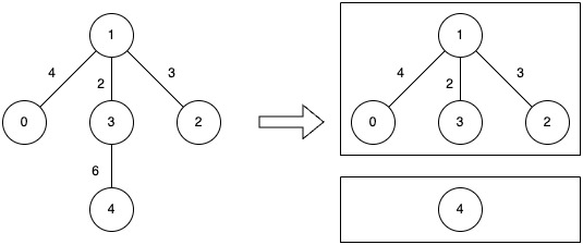
- Remove the edge between nodes 3 and 4 (weight 6).
- The resulting components have costs of 0 and 4, so the overall maximum cost is 4.
Example 2:
Input: n = 4, edges = [[0,1,5],[1,2,5],[2,3,5]], k = 1
Output: 5
Explanation:
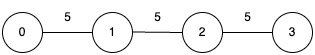
- No edge can be removed, since allowing only one component (
k = 1) requires the graph to stay fully connected. - That single component’s cost equals its largest edge weight, which is 5.
Constraints:
1 <n <= 5 * 10=40 <edges.length <= 10=5edges[i].length =3=0 <u=i=, v=i= < n=1 <w=i= <= 10=61 <k <= n=- The input graph is connected.
※ 4.1.1.2.1. Constraints and Edge Cases
<list constraints, input limits, or tricky edge cases here>
※ 4.1.1.2.2. My Solution (Code)
1: import heapq 2: from collections import defaultdict, deque 3: 4: class Solution: 5: │ def minCost(self, n: int, edges: List[List[int]], k: int) -> int: 6: │ │ """ 7: │ │ qns understanding: 8: │ │ - graph is a connected graph 9: │ │ - i have a list of edges and k k is the threshold for max number of connected components in the graph 10: │ │ - edges are really just u,v,w 11: │ │ - cost of component == max edge weight in that component ==> just have to keep track of max edge 12: │ │ 13: │ │ process of removal: 14: │ │ - can remove any edge from graph 15: │ │ - just needs to have at most k connected components 16: │ │ 17: │ │ 18: │ │ return: 19: │ │ - min possible value of MAX cost among all components after removal 20: │ │ 21: │ │ === 22: │ │ feels like a greedy thing needed, inputs imply some sort of linear approach 23: │ │ 24: │ │ == obs: 25: │ │ - any cut will break up a component into two components, we need to know the max edge after the cuts 26: │ │ - we care about cuts, at most k cuts 27: │ │ - we prioritise the cuts 28: │ │ 29: │ │ suspect it's a counting problem 30: │ │ """ 31: │ │ num_components = 1 32: │ │ node_to_gid = {} 33: │ │ adj = defaultdict(set) 34: │ │ 35: │ │ for u,v, w in edges: 36: │ │ │ node_to_gid[u] = num_components 37: │ │ │ node_to_gid[v] = num_components 38: │ │ │ 39: │ │ │ adj[u].add(v) 40: │ │ │ adj[v].add(u) 41: │ │ │ 42: │ │ pq = heapq([(-w, idx, u, v) for idx, (u, v, w) in enumerate(edges)]) # max heap, negated so that we can cut the biggest cost edge first 43: │ │ 44: │ │ def bfs(node, new_gid): 45: │ │ │ visited = {node} 46: │ │ │ queue = deque([node]) 47: │ │ │ while queue: 48: │ │ │ │ curr_node = queue.popleft() 49: │ │ │ │ node_to_gid[curr_node] = new_gid 50: │ │ │ │ for nei in adj[curr_node]: 51: │ │ │ │ │ if nei in visited: 52: │ │ │ │ │ │ continue 53: │ │ │ │ │ visited.add(nei) 54: │ │ │ │ │ queue.append(nei) 55: │ │ │ │ │ 56: │ │ while num_components < k: 57: │ │ │ # I wish to find good cuts 58: │ │ │ if not pq: 59: │ │ │ │ return 0 60: │ │ │ │ 61: │ │ │ best_cut = neg_w, idx, u, v = heapq.heappop(pq) 62: │ │ │ num_components += 1 63: │ │ │ adj[u].discard(v) 64: │ │ │ adj[v].discard(u) 65: │ │ │ # run a single bfs on one of them and update the gid 66: │ │ │ bfs(v, num_components) 67: │ │ │ 68: │ │ sorted(list(set(node_to_gid.values())) 69: │ │ 70: │ │ 71: # cut my losses at 31:59
Problems:
- we’re trying to remove edges greedily, but it doesn’t leverage binary search or union find to check feasibility efficiently
- the bfs use might become expensive
- current solution won’t handle the problem for large inputs based on the constraints which look almost linear-like
- some logical gaps:
- not evaluating if resulting max cost is minimal, just doing edge cuts
- bfs is wasteful, many re-processing done
1: import heapq 2: from collections import defaultdict, deque 3: 4: class UnionFind: 5: │ def __init__(self, n): 6: │ │ self.parent = list(range(n)) 7: │ │ self.rank = [0] * n 8: │ │ self.count = n # number of components 9: │ │ 10: │ def find(self, x): 11: │ │ """ 12: │ │ Finds the parent of a node, path compresses automatically 13: │ │ """ 14: │ │ if self.parent[x] != x: 15: │ │ │ self.parent[x] = self.find(self.parent[x]) 16: │ │ │ 17: │ │ return self.parent[x] 18: │ │ 19: │ def union(self, x, y): 20: │ │ """ 21: │ │ Unions x and y if they aren't already. 22: │ │ """ 23: │ │ rootx, rooty = self.find(x) , self.find(y) 24: │ │ 25: │ │ if rootx == rooty: 26: │ │ │ return 27: │ │ │ 28: │ │ # join them up, the one with the smaller rank goes to the one with the bigger rank: 29: │ │ if self.rank[rootx] > self.rank[rooty]: 30: │ │ │ self.parent[rooty] = rootx 31: │ │ │ 32: │ │ elif self.rank[rooty] > self.rank[rootx]: 33: │ │ │ self.parent[rootx] = rooty 34: │ │ │ 35: │ │ else: 36: │ │ │ self.parent[rooty] = rootx 37: │ │ │ self.rank[rootx] += 1 38: │ │ │ 39: │ │ self.count -= 1 40: │ │ return 41: │ │ 42: class Solution: 43: │ def minCost(self, n: int, edges: List[List[int]], k: int) -> int: 44: │ │ """ 45: │ │ We will binary search in the domain of the weights: 46: │ │ """ 47: │ │ if not edges: 48: │ │ │ return 0 49: │ │ max_edge = max(w for _,_,w in edges) 50: │ │ left, right = 0, max_edge 51: │ │ 52: │ │ def can_split(max_weight): 53: │ │ │ uf = UnionFind(n) # number of nodes 54: │ │ │ # join up edges if the edge is less than the max_weight chosen 55: │ │ │ for u, v, w in edges: 56: │ │ │ │ if w <= max_weight: 57: │ │ │ │ │ uf.union(u, v) 58: │ │ │ │ │ 59: │ │ │ return uf.count <= k 60: │ │ │ 61: │ │ ans = right # at least will be this, inclusive range 62: │ │ while left <= right: 63: │ │ │ mid = left + ((right - left) // 2) 64: │ │ │ if can_split(mid): 65: │ │ │ │ ans = mid # write it out first 66: │ │ │ │ right = mid - 1 # inclusive range 67: │ │ │ else: 68: │ │ │ │ left = mid + 1 69: │ │ │ │ 70: │ │ return ans
This works (though not optimal) but it’s alright. The key idea is that we need to track connected components and instead of trying to cut edges, we wish to build them up instead. That’s what the UF helper function is for.
The intuition here is that if we consider the MST of the graph. The MST connects ALL nodes with minimum total edge weight without cycles. If we want at most k connected components, we can partition the MST by removing the k - 1 largest weight edges (within the MST).
the max edge weight among the remaining components is minimised because the MST is minimum overall \(\implies\) the answer is the weight of the \(( k - 1 )^{th}\) largest edge in the MST after removing those edges
1: class UnionFind(): 2: │ def __init__(self, n): 3: │ │ self.parent = list(range(n)) 4: │ │ self.rank = [0] * n 5: │ │ 6: │ def find(self, x): 7: │ │ """ 8: │ │ Gets the parent of x: 9: │ │ """ 10: │ │ if self.parent[x] != x: 11: │ │ │ self.parent[x] = self.find(self.parent[x]) 12: │ │ │ 13: │ │ return self.parent[x] 14: │ │ 15: │ def union(self, x, y): 16: │ │ """ 17: │ │ Returns true if they were not joined before and are now joined. False otherwise. 18: │ │ """ 19: │ │ rootx, rooty = self.find(x), self.find(y) 20: │ │ if rootx == rooty: 21: │ │ │ return False 22: │ │ │ 23: │ │ # join up the smaller entity: 24: │ │ if self.rank[rootx] < self.rank[rooty]: 25: │ │ │ self.parent[rootx] = rooty 26: │ │ │ 27: │ │ elif self.rank[rooty] < self.rank[rootx]: 28: │ │ │ self.parent[rooty] = rootx 29: │ │ │ 30: │ │ else: 31: │ │ │ self.parent[rooty] = rootx 32: │ │ │ self.rank[rootx] += 1 33: │ │ │ 34: │ │ return True 35: │ │ 36: │ │ 37: class Solution: 38: │ def minCost(self, n: int, edges: List[List[int]], k: int) -> int: 39: │ │ """ 40: │ │ We build an MST with kruskal's method, then we know that it's 1 whole connected component. We try to remove k - 1 edges to create k connected components. 41: │ │ """ 42: │ │ uf = UnionFind(n) 43: │ │ edges.sort(key=lambda x:x[2]) 44: │ │ mst_edges = [] 45: │ │ 46: │ │ # build MST 47: │ │ for u, v, w in edges: 48: │ │ │ if uf.union(u, v): 49: │ │ │ │ mst_edges.append(w) 50: │ │ │ │ 51: │ │ if k == 1: 52: │ │ │ return max(mst_edges) if mst_edges else 0 53: │ │ │ 54: │ │ # now we do the edge removals for k - 1 largest edges to give k connected components 55: │ │ mst_edges.sort(reverse=True) 56: │ │ for _ in range(k - 1): 57: │ │ │ if mst_edges: 58: │ │ │ │ mst_edges.pop(0) 59: │ │ │ │ 60: │ │ return max(mst_edges) if mst_edges else 0
※ 4.1.1.2.3. My Approach/Explanation
Not great
※ 4.1.1.2.4. My Learnings/Questions
- Key Intuition:
- so we know that it’s got something to do with connected component tracking so a union find approach makes sense \(\implies\) have to find out how to use a union find here.
- we also know that we’re trying to do some sort of min maxing and a greedy approach might make sense for us here.
We can phrase it like a binary search: W, the min possible max edge weight is what we want to find. We remove all edges with weights > W and we should be getting at most k components
Since the search space along the edge weights can be ordered \(\implies\) consider binary search.
Binary search in the range [0, maxWeight], for each mid, W, build a union find ds, connect only edges with weight <= W. Then count the number of connected components formed. Search appropriately.
- we can also consider MST approaches when thinking about connected graphs and making cuts to it to create connected components.
※ 4.1.1.3. DONE Q3: Process String with Special Operations II (3614) failed virtual_simulation arrays simulation
You are given a string s consisting of lowercase English letters and
the special characters: '*', '#', and '%'.
You are also given an integer k.
Build a new string result by processing s according to the following
rules from left to right:
- If the letter is a lowercase English letter append it to
result. - A
'*'removes the last character fromresult, if it exists. - A
'#'duplicates the currentresultand appends it to itself. - A
'%'reverses the currentresult.
Return the k=^{=th} character of the final string result. If k is
out of the bounds of result, return '.'.
Example 1:
Input: s = “a#b%*”, k = 1
Output: “a”
Explanation:
i |
s[i] |
Operation | Current result |
|---|---|---|---|
| 0 | 'a' |
Append 'a' |
"a" |
| 1 | '#' |
Duplicate result |
"aa" |
| 2 | 'b' |
Append 'b' |
"aab" |
| 3 | '%' |
Reverse result |
"baa" |
| 4 | '*' |
Remove the last character | "ba" |
The final result is "ba". The character at index k = 1 is 'a'.
Example 2:
Input: s = “cd%#*#”, k = 3
Output: “d”
Explanation:
i |
s[i] |
Operation | Current result |
|---|---|---|---|
| 0 | 'c' |
Append 'c' |
"c" |
| 1 | 'd' |
Append 'd' |
"cd" |
| 2 | '%' |
Reverse result |
"dc" |
| 3 | '#' |
Duplicate result |
"dcdc" |
| 4 | '*' |
Remove the last character | "dcd" |
| 5 | '#' |
Duplicate result |
"dcddcd" |
The final result is "dcddcd". The character at index k = 3 is
'd'.
Example 3:
Input: s = “z*#”, k = 0
Output: “.”
Explanation:
i |
s[i] |
Operation | Current result |
|---|---|---|---|
| 0 | 'z' |
Append 'z' |
"z" |
| 1 | '*' |
Remove the last character | "" |
| 2 | '#' |
Duplicate the string | "" |
The final result is "". Since index k = 0 is out of bounds, the
output is '.'.
Constraints:
1 <s.length <= 10=5sconsists of only lowercase English letters and special characters'*','#', and'%'.0 <k <= 10=15- The length of
resultafter processingswill not exceed10=^{=15}.
※ 4.1.1.3.1. Constraints and Edge Cases
<list constraints, input limits, or tricky edge cases here>
※ 4.1.1.3.2. My Solution (Code)
1: from collections import deque 2: class Solution: 3: │ def processStr(self, s: str, k: int) -> str: 4: │ │ """ 5: │ │ naive approach will violate memory bounds, that's why we shall look for amortisation options 6: │ │ """ 7: │ │ res = [] 8: │ │ for char in s: 9: │ │ │ if char == "*" and res: 10: │ │ │ │ res.pop() 11: │ │ │ │ continue 12: │ │ │ if char == "#" and res: 13: │ │ │ │ res.extend(res) 14: │ │ │ │ continue 15: │ │ │ if char == "%" and res: 16: │ │ │ │ for i in range(len(res) // 2): 17: │ │ │ │ │ # inplace swap: 18: │ │ │ │ │ a, b = i, len(res) - 1 - i 19: │ │ │ │ │ res[a], res[b] = res[b], res[a] 20: │ │ │ │ continue 21: │ │ │ │ 22: │ │ │ if char.islower(): 23: │ │ │ │ res.append(char) 24: │ │ │ │ 25: │ │ if not (0 <= k < len(res)): 26: │ │ │ return "." 27: │ │ │ 28: │ │ return res[k] 29: │ │ 30: │ │ 31: │ │ 32: │ │ 33: │ │ 34: │ │ 35: │ │ # res = deque([]) 36: │ │ # is_reverse = False 37: │ │ 38: │ │ # for char in s: 39: │ │ # # deletion: 40: │ │ # if char == "*" and res: 41: │ │ # if is_reverse: 42: │ │ # res.popleft() 43: │ │ # else: 44: │ │ # res.pop() 45: │ │ # continue 46: │ │ 47: │ │ # # duplication: 48: │ │ # if char == "#": 49: │ │ # # res += res 50: │ │ # res.extend(res) 51: │ │ # continue 52: │ │ 53: │ │ # # reversing: 54: │ │ # if char == "%": 55: │ │ # is_reverse = not is_reverse 56: │ │ # continue 57: │ │ 58: │ │ # if is_reverse: 59: │ │ # res.appendleft(char) 60: │ │ # else: 61: │ │ # res.append(char) 62: │ │ 63: │ │ # choice_idx = k if not is_reverse else len(res) - k - 1 64: │ │ # if not (0 <= choice_idx < len(res)): 65: │ │ # return "." 66: │ │ 67: │ │ # return res[choice_idx] 68: │ │ 69: │ │ 70: │ │ # # res = [] 71: │ │ # # is_reverse = False 72: │ │ 73: │ │ # # DEL = '-' 74: │ │ 75: │ │ # # for char in s: 76: │ │ # # # deletion 77: │ │ # # if char == "*": 78: │ │ # # if not res: 79: │ │ # # continue 80: │ │ # # deletion_idx = 0 if is_reverse else -1 81: │ │ # # while not_found_deletion_idx:=(res[deletion_idx] == DEL): 82: │ │ # # next_idx = deletion_idx + 1 if is_reverse else deletion_idx - 1 83: │ │ # # deletion_idx = next_idx 84: │ │ # # if not (0 <= next_idx < len(res)): 85: │ │ # # break 86: │ │ 87: │ │ # # if not (0 <= deletion_idx < len(res)): # out of bounds, nothign left to do. 88: │ │ # # continue 89: │ │ 90: │ │ # # res[deletion_idx] = DEL 91: │ │ # # # duplicate 92: │ │ # # if char == "#": 93: │ │ # # pruned = [c for c in res if c != DEL] 94: │ │ # # res = pruned + pruned 95: │ │ # # continue 96: │ │ # # # flip 97: │ │ # # if char == "%": 98: │ │ # # is_reverse = not is_reverse 99: │ │ # # continue 100: │ │ 101: │ │ # # if not is_reverse: 102: │ │ # # res.append(char) 103: │ │ # # else: 104: │ │ 105: │ │ # return res[k] if k < len(res) else "."
This is a reverse simulation that we need to do, we shall do it via a 2 pass approach. First one is to find out the final length of the output string, then we will use the inverse of each process and do some logic there.
1: class Solution: 2: │ def processStr(self, s: str, k: int) -> str: 3: │ │ """ 4: │ │ This is virtual simulation of the string operations, instead of directly simulating it. 5: │ │ We won't construct the string and operate on it, we will work backwards, doing the inverse operations. 6: │ │ We shall do 2 passes: 7: │ │ 1. find the final length, early return if not satisfactory 8: │ │ 2. in reverse order of the input, we carry out inverse operations. we can early return when the char count matches k. 9: │ │ """ 10: │ │ # first pass: final length calculation 11: │ │ size = 0 12: │ │ for c in s: 13: │ │ │ if c.islower(): 14: │ │ │ │ size += 1 15: │ │ │ elif c == "*" and size > 0: # remover, pops 1 out 16: │ │ │ │ size -= 1 17: │ │ │ elif c == "#": # duplicator 18: │ │ │ │ size *= 2 19: │ │ │ │ 20: │ │ # early returns if out of bounds index 21: │ │ if not (0 <= k < size): 22: │ │ │ return '.' 23: │ │ │ 24: │ │ # 2nd pass, inverse simulation: 25: │ │ for c in reversed(s): 26: │ │ │ if c.islower(): 27: │ │ │ │ size -= 1 28: │ │ │ │ # found the char: 29: │ │ │ │ if k == size: 30: │ │ │ │ │ return c 31: │ │ │ elif c == "*": # inverse of poping is pushing 32: │ │ │ │ size += 1 33: │ │ │ elif c == "#": # inverse of doubling is halving, but need to be careful if we need to rotate k 34: │ │ │ │ size //= 2 35: │ │ │ │ if k >= size: # is in theright half 36: │ │ │ │ │ k -= size 37: │ │ │ elif c == "%": # need to flip it: 38: │ │ │ │ k = size - 1 - k 39: │ │ │ │ 40: │ │ return "."
※ 4.1.1.3.3. My Approach/Explanation
This is a simulation question, we will MLE so we need to do a virtual simulation without actually manipulating the string.
The optimal solution is so elegant.
※ 4.1.1.3.4. My Learnings/Questions
- TRICK/STYLE: string simulations / simulations in general, if we face an MLE then we need to consider how to do virtual simulations for this.
※ 4.1.1.3.5. [Optional] Additional Context
※ 4.1.1.4. TODO Q4: Longest Palindromic Path in Graph (3615) wtf
You are given an integer n and an undirected graph with n nodes
labeled from 0 to n - 1 and a 2D array edges, where
edges[i] = [u=_{=i}=, v=i=]= indicates an edge between nodes
u=_{=i} and v=_{=i}.
You are also given a string label of length n, where label[i] is
the character associated with node i.
You may start at any node and move to any adjacent node, visiting each node at most once.
Return the maximum possible length of a palindrome that can be formed by visiting a set of unique nodes along a valid path.
Example 1:
Input: n = 3, edges = [[0,1],[1,2]], label = “aba”
Output: 3
Explanation:
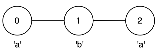
- The longest palindromic path is from node 0 to node 2 via node 1,
following the path
0 → 1 → 2forming string"aba". - This is a valid palindrome of length 3.
Example 2:
Input: n = 3, edges = [[0,1],[0,2]], label = “abc”
Output: 1
Explanation:
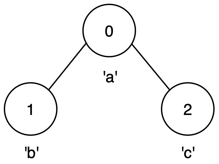
- No path with more than one node forms a palindrome.
- The best option is any single node, giving a palindrome of length 1.
Example 3:
Input: n = 4, edges = [[0,2],[0,3],[3,1]], label = “bbac”
Output: 3
Explanation:
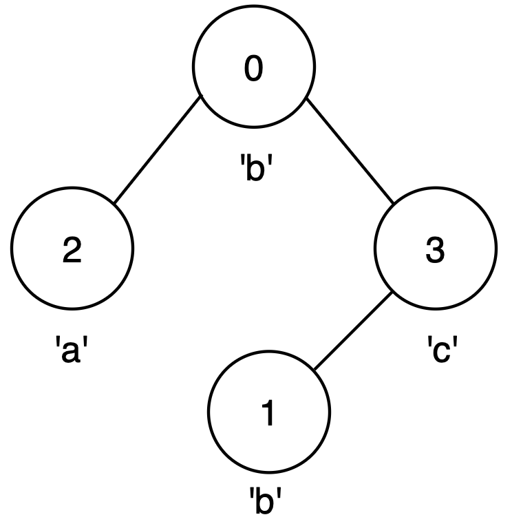
- The longest palindromic path is from node 0 to node 1, following the
path
0 → 3 → 1, forming string"bcb". - This is a valid palindrome of length 3.
Constraints:
1 <n <= 14=n - 1 <edges.length <= n * (n - 1) / 2=edges[i] =[u=i=, v=i=]=0 <u=i=, v=i= <= n - 1=u=_{=i}= != v=ilabel.length =n=labelconsists of lowercase English letters.- There are no duplicate edges.
※ 4.1.1.4.1. Constraints and Edge Cases
<list constraints, input limits, or tricky edge cases here>
※ 4.1.1.4.2. My Solution (Code)
I’m not going to implement this directly yet, just going to essay plan it.
1: class Solution: 2: │ def maxLen(self, n: int, edges: List[List[int]], label: str) -> int: 3: │ │ """ 4: │ │ Essay plan: 5: │ │ 6: │ │ The rough idea is to do traversals while adhering to some contraints. The contraint is that we're building palindromes. If we can't build then we need find other ways. 7: │ │ 8: │ │ The expand from middle approach for palindrome finding comes to mind. 9: │ │ As we do a BFS, we are going outward, we need to be able to keep track of palindromes-building for the neighbours. ==> so the palindrome property becomes a two ended expansion problem 10: │ │ 11: │ │ Analysing the inputs: 12: │ │ 1. small graph size might mean it's exponential approach with pruning or DP of some sort 13: │ │ """
※ 4.1.1.4.3. My Approach/Explanation
<briefly explain your reasoning, algorithm, and why you chose it>
※ 4.1.1.4.4. My Learnings/Questions
<what did you learn? any uncertainties or questions?>
※ 4.1.1.4.5. Prompt for GPT Evaluation
Please do the following:
- Evaluate the correctness of my solution. Are there any logical or edge case errors?
- Analyze the time and space complexity of my code.
- Suggest improvements in code style, efficiency, or clarity.
- Compare my approach to the optimal solution (if different).
- Provide a sample optimal solution (if mine is not optimal).
- Point out any Pythonic (or language-specific) improvements.
Are there any completely different approaches to this problem?
- e.g something that uses a completely different data structure
If so, then help me gain the intuition for it and show the code clearly
- Answer my specific questions (if any are listed above).
※ 4.1.1.4.6. Prompt for GPT Evaluation (with Greedy)
Please do the following:
- Evaluate the correctness of my solution. Are there any logical or edge case errors?
- Analyze the time and space complexity of my code.
- Suggest improvements in code style, efficiency, or clarity.
- Compare my approach to the optimal solution (if different).
- Provide a sample optimal solution (if mine is not optimal).
- Point out any Pythonic (or language-specific) improvements.
Are there any completely different approaches to this problem?
- e.g something that uses a completely different data structure
If so, then help me gain the intuition for it and show the code clearly
- Answer my specific questions (if any are listed above).
ALso help me evaluate this in the context of greedy algorithms, ensuring that a good framework of presenting this problem into a greedy algo is given / understood.
※ 4.1.1.4.7. Prompt for GPT Evaluation (with DP)
Please do the following:
- Evaluate the correctness of my solution. Are there any logical or edge case errors?
- Analyze the time and space complexity of my code.
- Suggest improvements in code style, efficiency, or clarity.
- Compare my approach to the optimal solution (if different).
- Provide a sample optimal solution (if mine is not optimal).
- Point out any Pythonic (or language-specific) improvements.
Are there any completely different approaches to this problem?
- e.g something that uses a completely different data structure
If so, then help me gain the intuition for it and show the code clearly
- Answer my specific questions (if any are listed above).
ALso help me evaluate this in the context of greedy algorithms, ensuring that a good framework of presenting this problem into a greedy algo is given / understood.
Additionally, use my notes for Dynamic Programming and use the recipes that are here.
Recipe to define a solution via DP
[Generate Naive Recursive Algo]
Characterise the structure of an optimal solution \(\implies\) what are the subproblems? \(\implies\) are they independent subproblems? \(\implies\) how many subproblems will there be?
- Recursively define the value of an optimal solution \(\implies\) does this have the overlapping sub-problems property? \(\implies\) what’s the cost of making a choice? \(\implies\) how many ways can I make that choice?
- Compute value of an optimal solution
- Construct optimal solution from computed information Defining things
- Optimal Substructure:
A problem exhibits “optimal substructure” if an optimal solution to the problem contains within it optimal solutions to subproblems.
Elements of Dynamic Programming: Key Indicators of Applicability [1] Optimal Sub-Structure Defining “Optimal Substructure” A problem exhibits optimal substructure if an optimal solution to the problem contains within it optimal solutions to sub-problems.
- typically a signal that DP (or Greedy Approaches) will apply here.
- this is something to discover about the problem domain Common Pattern when Discovering Optimal Substructure
solution involves making a choice e.g. choosing an initial cut in the rod or choosing what k should be for splitting the matrix chain up
\(\implies\) making the choice also determines the number of sub-problems that the problem is reduced to
- Assume that the optimal choice can be determined, ignore how first.
- Given the optimal choice, determine what the sub-problems looks like \(\implies\) i.e. characterise the space of the subproblems
- keep the space as simple as possible then expand
typically the substructures vary across problem domains in 2 ways:
[number of subproblems]
how many sub-problems does an optimal solution to the original problem use?
- rod cutting:
# of subproblems = 1(of size n-i) where i is the chosen first cut lengthmatrix split:
# of subproblems = 2(left split and right split)[number of subproblem choices]
how many choices are there when determining which subproblems(s) to use in an optimal solution. i.e. now that we know what to choose, how many ways are there to make that choice?
- rod cutting: # of choices for i = length of first cut,
nchoices- matrix split: # of choices for where to split (idx k) =
j - iNaturally, this is how we analyse the runtime:
# of subproblems * # of choices @ each sub-problem- Reason to yourself if and how solving the subproblems that are used in an optimal solution means that the subproblem-solutions are also optimal. This is typically done via the
cut-and-paste argument.Caveat: Subproblems must be
independent
- “independent subproblems”
- solution to one subproblem doesn’t affect the solution to another subproblem for the same problem
example: Unweighted Shortest Path (independent subproblems) vs Unweighted Longest Simple Path (dependent subproblems)
Consider graph \(G = (V,E)\) with vertices \(u,v \notin V\)
- Unweighted shortest path: we want to find path \(u\overset{p}{\leadsto}v\) then we can break it down into subpaths \(u\overset{p1}{\leadsto}w\overset{p2}{\leadsto}v\) (optimal substructure). If path, p, is optimal from \(u\leadsto{v}\) then p1 must be shortest path from \(u\leadsto{w}\) and likewise p2 must be shortest path from \(w\leadsto{v}\) (cut-and-paste argument) Here, we know that the subproblems are independent.
- Unweighted Longest Simple Path: the subproblems can have paths that overlap (not subproblem overlap), hence it’s not independent because the vertices that appear can appear in the solution to the second subproblem
Terminology: Optimal substruture vs optimal solution optimal substructure is a property that enables efficient computation of the optimal value, while the solution is the specific configuration that yields that optimal value
You’re right that in dynamic programming algorithms for optimization problems, the goal is usually to find an optimal solution rather than the unique optimal solution. Here’s how the optimal substructure and the actual solution differ:
### Optimal Substructure
The optimal substructure refers to the property that the optimal solution to a problem can be constructed from the optimal solutions to its subproblems. This means that if we know the optimal solutions to the subproblems, we can efficiently determine the optimal solution to the overall problem.
For example, in the rod cutting problem, if we know the maximum revenue for rods of length 1 to n-1, we can efficiently determine the maximum revenue for a rod of length n by considering cutting the rod at each possible length and taking the maximum revenue.
### The Solution
The actual solution, on the other hand, refers to the specific configuration or set of choices that yields the optimal value. In the rod cutting problem, the solution would be the specific way to cut the rod that results in the maximum revenue.
The key difference is that the optimal substructure allows us to efficiently compute the optimal value, but it doesn’t necessarily specify the exact solution. There may be multiple solutions that yield the same optimal value.
For example, in the rod cutting problem, there may be multiple ways to cut the rod that result in the same maximum revenue. The optimal substructure allows us to efficiently compute the maximum revenue, but it doesn’t specify which particular cutting configuration to choose.
So in summary, the optimal substructure is a property that enables efficient computation of the optimal value, while the solution is the specific configuration that yields that optimal value. Dynamic programming algorithms leverage the optimal substructure to efficiently compute the optimal value, but the actual solution may not be uniquely determined.
Citations: [1] https://library.fiveable.me/key-terms/programming-for-mathematical-applications/optimal-substructure [2] https://afteracademy.com/blog/optimal-substructure-and-overlapping-subproblems/ [3] https://www.geeksforgeeks.org/optimal-substructure-property-in-dynamic-programming-dp-2/ [4] https://labuladong.gitbook.io/algo-en/i.-dynamic-programming/optimalsubstructure [5] https://stackoverflow.com/questions/33563230/optimal-substructure-in-dynamic-programing [6] https://en.wikipedia.org/wiki/Optimal_substructure [7] https://www.cs.cmu.edu/~15451-f22/lectures/lec09-dp1.pdf [8] https://www.javatpoint.com/optimal-substructure-property
[2] Overlapping Sub-Problems
- DP should be disambiguated from Divide & Conquer:
- for Divide&Conquer, choosing a division point generates brand new problems that likely don’t overlap
- for DP, the space of sub-problems is small and hence if done purely recursively, the same operations get computed multiple times
[Practical point] Reconstructing an optimal solution Since one way to look at DP is table-filling, we typically have:
- table of costs
- table of optimal choices
the table of optimal choices can be built from the table of costs, but we want to avoid recalculating the optimal choices
Memoisation as an alternative
- the textbook used sees this as an alternative and memoised tables as the aux DS for recursive, top-down approaches
- memoisation also exploits the observation that the space of the subproblems is small and hence overlapping
Common Misconceptions Here are some common misconception, based on what perplexity says
Based on the search results, here are some of the common misconceptions that learners have about dynamic programming:
## 1. Misconceptions about the Definition and Purpose of Dynamic Programming
- Thinking that recursion and dynamic programming are explicitly different concepts[3].
- Believing that dynamic programming is exclusively used to solve optimization problems[3].
## 2. Misconceptions about the Optimal Substructure Property
- Assuming that the optimal solution to a problem can be constructed from any combination of optimal solutions to its subproblems, rather than specific optimal solutions to the right subproblems[1][2].
- Thinking that the optimal solution to a problem can be constructed from optimal solutions to unrelated subproblems[4].
## 3. Misconceptions about Memoization and Tabulation
- Failing to recognize that memoization (top-down) and tabulation (bottom-up) are two different implementation strategies for dynamic programming[1][2].
- Believing that memoization always involves recursion and tabulation always involves iteration[1][2].
## 4. Misconceptions about the Filling Order of the DP Table
- Assuming that the DP table must always be filled in a specific order (e.g., always from small to big cases), without understanding that the order depends on the problem’s dependencies and constraints[1][2][4].
## 5. Misconceptions about the Relationship between Subproblems
- Thinking that the solutions to all subproblems are needed to solve the original problem, rather than understanding that only specific optimal solutions to the right subproblems are needed[1][2].
## 6. Misconceptions about the Efficiency of Dynamic Programming
- Believing that dynamic programming always leads to polynomial-time algorithms, without understanding that it can sometimes only slightly improve the exponential-time complexity[4].
Understanding and addressing these common misconceptions can help learners develop a more accurate and comprehensive understanding of dynamic programming and its applications.
Citations: [1] https://dl.acm.org/doi/10.1145/3159450.3159528 [2] https://dl.acm.org/doi/abs/10.1145/3159450.3159528 [3] https://ics.uci.edu/~mikes/papers/Student_Misconceptions_Dynamic_Programming.pdf [4] https://www.cs.cmu.edu/~15451-f22/lectures/lec09-dp1.pdf [5] https://www.reddit.com/r/compsci/comments/er05hn/help_me_wrap_my_head_around_dynamic_programming/ [6] https://yourbasic.org/algorithms/dynamic-programming-explained/ [7] https://stackoverflow.com/questions/33563230/optimal-substructure-in-dynamic-programing [8] https://lec.inf.ethz.ch/DA/2020/slides/daLecture13.en.pdf
Greedy Algos vs DP When comparing greedy strategies and dynamic programming (DP), it’s essential to understand how they differ in methodology, application, and the nature of the problems they solve. Both approaches involve identifying optimal substructures, but they apply this concept in distinct ways. Here’s a detailed disambiguation based on the search results:
### 1. Definition and Approach
- Greedy Strategy:
- A greedy algorithm makes the most optimal choice at each step with the hope that these local optimum choices will lead to a global optimum solution. It does not consider the overall impact of the current choice on future decisions.
- Greedy algorithms are typically simpler and faster to implement, as they do not require storing results of subproblems. However, they do not guarantee an optimal solution for all problems.
- Dynamic Programming:
- Dynamic programming is a technique used to solve complex problems by breaking them down into simpler subproblems. It is based on the principles of optimal substructure and overlapping subproblems.
- DP guarantees an optimal solution by considering all possible cases and storing the results of subproblems to avoid redundant computations. This can lead to higher time and space complexity compared to greedy algorithms.
### 2. Optimal Substructure
- Greedy Algorithms:
- Greedy algorithms rely on the greedy choice property, which means that a locally optimal choice leads to a globally optimal solution. However, this property does not hold for all problems, which is why greedy algorithms may fail to find the optimal solution in some cases.
- Dynamic Programming:
- Dynamic programming explicitly uses the optimal substructure property, where an optimal solution to a problem can be constructed from optimal solutions of its subproblems. DP ensures that all relevant subproblems are considered, leading to a guaranteed optimal solution.
### 3. Subproblem Reuse
- Greedy Strategy:
- Greedy algorithms typically do not reuse solutions to subproblems. Each decision is made independently based on the current state without revisiting previous choices.
- Dynamic Programming:
- DP explicitly solves and caches solutions to overlapping subproblems. This reuse of subproblem solutions is a key feature of dynamic programming, allowing for efficient computation.
### 4. Complexity and Efficiency
- Greedy Algorithms:
- Greedy algorithms are generally more efficient in terms of time complexity due to their straightforward approach. They often run in linear or logarithmic time, depending on the problem.
- They are suitable for problems where local optimization leads to global optimization, such as in minimum spanning trees or certain shortest path problems.
- Dynamic Programming:
- DP can be less efficient than greedy algorithms in terms of time complexity, especially if every possible solution is computed. However, proper use of memoization can mitigate this.
- DP is applicable to problems with overlapping subproblems and optimal substructure, such as the Fibonacci sequence, longest common subsequence, or knapsack problems.
### 5. Examples
- Greedy Algorithms:
- Common examples include:
- Fractional Knapsack Problem: Where you can take fractions of items.
- Minimum Spanning Tree: Algorithms like Prim’s and Kruskal’s.
- Huffman Coding: For optimal prefix codes.
- Dynamic Programming:
- Common examples include:
- 0/1 Knapsack Problem: Where you cannot take fractions of items.
- Longest Common Subsequence: Finding the longest subsequence present in both sequences.
- Matrix Chain Multiplication: Finding the most efficient way to multiply a given sequence of matrices.
### Conclusion
In summary, while both greedy strategies and dynamic programming involve the concept of optimal substructure, they differ significantly in their approach to problem-solving. Greedy algorithms make decisions based on local optimality without revisiting previous choices, whereas dynamic programming systematically considers all possible subproblems and their solutions to ensure a globally optimal result. Understanding these differences allows for better problem-solving strategies and the appropriate application of each method based on the problem’s characteristics.
Citations: [1] https://www.boardinfinity.com/blog/greedy-vs-dp/ [2] https://www.shiksha.com/online-courses/articles/difference-between-greedy-and-dynamic-programming-blogId-158053 [3] https://www.interviewbit.com/blog/difference-between-greedy-and-dynamic-programming/ [4] https://stackoverflow.com/questions/16690249/what-is-the-difference-between-dynamic-programming-and-greedy-approach [5] https://www.geeksforgeeks.org/greedy-approach-vs-dynamic-programming/ [6] https://byjus.com/gate/difference-between-greedy-approach-and-dynamic-programming/ [7] https://www.cs.cmu.edu/~15451-f22/lectures/lec09-dp1.pdf [8] https://ics.uci.edu/~mikes/papers/Student_Misconceptions_Dynamic_Programming.pdf
General Takeaways Bottom-up vs Top-Down
- we can use a subproblem graph to show the relationship with the subproblems ==> diff b/w bottom up and top-down is how these deps are handled (recursive-called or soundly iterated with a proper direction)
- aysymptotic runtime is pretty similar since both solve similar \(\Omega(n^{2})\)
- Bottom up:
- basically considers order at which the subproblems are solved
- because of the ordered way of solving the smaller sub-problems first, there’s no need for recursive calls and code can be iterative entirely
- so no overhead from function calls
- no chance of stack overflow
- benefits from data-locality
- a way to see the vertices of the subproblem graph such that the subproblems y-adjacent to a given subproblem x is solved before subproblem x is solved
※ 4.1.1.4.8. [Optional] Additional Context
<e.g., “I struggled with X”, “I want to know about alternative algorithms”, etc.>
※ 4.1.2. DONE Weekly Contest [459]
※ 4.1.2.1. Retro
※ 4.1.2.2. DONE Q1: Check Divisibility by Digit Sum and Product (3622)
You are given a positive integer n. Determine whether n is divisible
by the sum of the following two values:
- The digit sum of
n(the sum of its digits). - The digit product of
n(the product of its digits).
Return true if n is divisible by this sum; otherwise, return
false.
Example 1:
Input: n = 99
Output: true
Explanation:
Since 99 is divisible by the sum (9 + 9 = 18) plus product (9 * 9 = 81) of its digits (total 99), the output is true.
Example 2:
Input: n = 23
Output: false
Explanation:
Since 23 is not divisible by the sum (2 + 3 = 5) plus product (2 * 3 = 6) of its digits (total 11), the output is false.
Constraints:
1 <n <= 10=6
※ 4.1.2.2.1. Constraints and Edge Cases
Nothing fancy here.
※ 4.1.2.2.2. My Solution (Code)
1: class Solution: 2: │ def checkDivisibility(self, n: int) -> bool: 3: │ │ digits = [int(char) for char in str(n)] 4: │ │ 5: │ │ prod = 1 6: │ │ for d in digits: 7: │ │ │ prod *= d 8: │ │ │ 9: │ │ return n % (sum(digits) + prod) == 0
1: from math import prod 2: 3: class Solution: 4: │ def checkDivisibility(self, n: int) -> bool: 5: │ │ digits = [int(d) for d in str(n)] 6: │ │ return n % (sum(digits) + prod(digits)) == 0
※ 4.1.2.2.3. My Approach/Explanation
I think in these easy cases, just going for something that works is more important.
So I just went with the naive solution.
Burned some time because didn’t read the thing right on what is the divisor and what is the other operand though.
※ 4.1.2.2.4. My Learnings/Questions
- the digit stripping method is clean:
[ int(d) for d in str(int)] - better to get the naive solution out first
※ 4.1.2.2.5. [Optional] Additional Context
<e.g., “I struggled with X”, “I want to know about alternative algorithms”, etc.>
※ 4.1.2.3. DONE Q2: Count Number of Trapezoids I (3623) running_multiplication space_optimisation product_of_sum
You are given a 2D integer array points, where
points[i] = [x=_{=i}=, y=i=]= represents the coordinates of the
i=^{=th} point on the Cartesian plane.
A horizontal trapezoid is a convex quadrilateral with at least one pair of horizontal sides (i.e. parallel to the x-axis). Two lines are parallel if and only if they have the same slope.
Return the number of unique horizontal trapezoids that can be
formed by choosing any four distinct points from points.
Since the answer may be very large, return it modulo 10=^{=9}= + 7=.
Example 1:
Input: points = [[1,0],[2,0],[3,0],[2,2],[3,2]]
Output: 3
Explanation:
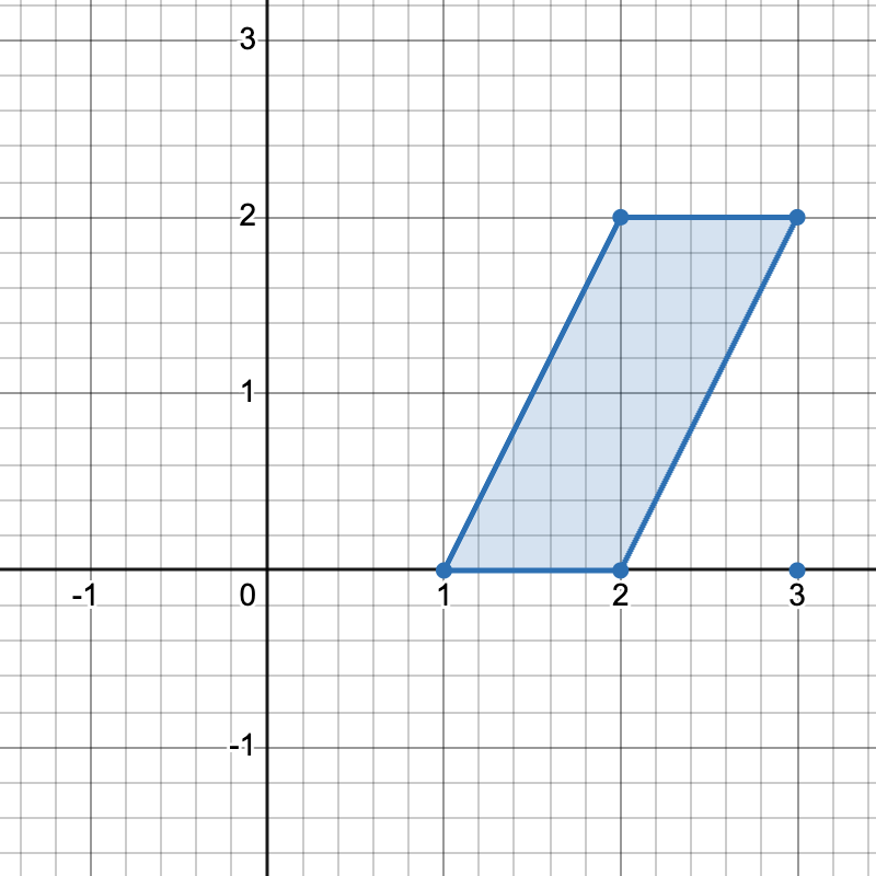
There are three distinct ways to pick four points that form a horizontal trapezoid:
- Using points
[1,0],[2,0],[3,2], and[2,2]. - Using points
[2,0],[3,0],[3,2], and[2,2]. - Using points
[1,0],[3,0],[3,2], and[2,2].
Example 2:
Input: points = [[0,0],[1,0],[0,1],[2,1]]
Output: 1
Explanation:
There is only one horizontal trapezoid that can be formed.
Constraints:
4 <points.length <= 10=5–10=^{=8}= <= x=i=, y=i= <= 10=8- All points are pairwise distinct.
※ 4.1.2.3.1. Constraints and Edge Cases
- all the points are pairwise distinct, so we don’t need to care about two different points having the same coordinates. This means that there are no duplicates for us to be worried about.
※ 4.1.2.3.2. My Solution (Code)
1: from collections import defaultdict 2: 3: class Solution: 4: │ def countTrapezoids(self, points: List[List[int]]) -> int: 5: │ │ """ 6: │ │ 1. counting problem, seraching for number of pairs of horizontal sides (identifiable via the y-axis intercepts) 7: │ │ 8: │ │ 2. choosing any 4 distinct points ==> large numbers ==> do a mod at each iteration 9: │ │ 10: │ === 11: │ 12: │ 1. preprocess, index it via the y values 13: │ │ """ 14: │ │ MOD = 10**9 + 7 15: │ │ # index points via y values, allow duplicates 16: │ │ level_to_points = defaultdict(list) 17: │ │ for x, y in points: 18: │ │ │ level_to_points[y].append((x, y)) 19: │ │ │ 20: │ │ # consider y1, y2, we have to pick 2 points from y1 and 2 points from y2 21: │ │ # we can prebuild the num_pairs 22: │ │ # points in the same level 23: │ │ def get_num_pairs(points): 24: │ │ │ count = 0 25: │ │ │ for i in range(len(points)): 26: │ │ │ │ for j in range(i): 27: │ │ │ │ │ xi, yi = points[i] 28: │ │ │ │ │ xj, yj = points[j] 29: │ │ │ │ │ if (xi == xj): 30: │ │ │ │ │ │ continue 31: │ │ │ │ │ count += 1 32: │ │ │ │ │ 33: │ │ │ return count 34: │ │ │ 35: │ │ level_pairs = [(get_num_pairs(points) % MOD) for points in level_to_points.values()] 36: │ │ total = 0 37: │ │ 38: │ │ for i in range(len(level_pairs)): 39: │ │ │ for j in range(i): 40: │ │ │ │ total += (level_pairs[i] * level_pairs[j]) % MOD 41: │ │ │ │ 42: │ │ return total
The approach seems to be right, but we need to optimise this further.
The pair counting is slow right now because we’re doing a double for loop that runs in \(O(n ^{2})\) time. We try to optimise that first. We could try to do a frequency count for that actually.
1: from collections import defaultdict 2: 3: class Solution: 4: │ def countTrapezoids(self, points: List[List[int]]) -> int: 5: │ │ """ 6: │ │ this is a counting exercise, we first group together by same y value 7: │ │ 8: │ │ then we can find out the number of pairs that we can form for each y value (level). 9: │ │ 10: │ │ Finally, it's about doing a sum of productpairs, for which we do some math hacks 11: │ │ """ 12: │ │ MOD = (10 ** 9) + 7 13: │ │ 14: │ │ level_to_points = defaultdict(list) 15: │ │ for x, y in points: 16: │ │ │ level_to_points[y].append((x, y)) 17: │ │ │ 18: │ │ level_pairs = [((len(points) * (len(points) - 1)) // 2) % MOD 19: │ │ │ │ │ │ for points in level_to_points.values()] 20: │ │ total_pairs_sum = sum(level_pairs) % MOD 21: │ │ total_pairs_sq_sum = sum( (x * x) % MOD for x in level_pairs) % MOD 22: │ │ inv2 = pow(2, MOD - 2, MOD) # params: base, exponent, modulus 23: │ │ total = ( 24: │ │ │ ((total_pairs_sum * total_pairs_sum) - total_pairs_sq_sum) 25: │ │ │ │* inv2 26: │ │ │ │% MOD) 27: │ │ │ │ 28: │ │ return total
I think the math here is non-obvious. Basically we want the sum of pair products and for that it uses ta convoluted way of doing sum of pairs and the square of this and then using some algebra for this.
There’s a useful math hack here:
- to get the sum of products, we can
Using this will allow us to avoid doing calculations iteratively and we can just get values via arithmetic.
The equation
\[
(\sum x_i)^2 = \sum x_i^2 + 2 \sum_{i
comes directly from the algebraic expansion of the square of a sum. Here’s how we come up with it, step-by-step:
Starting Point: Square of a sum
\[
(\sum_{i=1}^n x_i)^2 = (x_1 + x_2 + \cdots + x_n)^2
\]
Expand the square
Using distributive property, multiplication distributes over addition:
\[
= (x_1 + x_2 + \cdots + x_n)(x_1 + x_2 + \cdots + x_n)
\]
Multiply each term in the first sum by each term in the second sum:
\[
= x_1x_1 + x_1x_2 + \cdots + x_1x_n + x_2x_1 + x_2x_2 + \cdots + x_2x_n + \cdots + x_nx_1 + x_nx_2 + \cdots + x_nx_n
\]
Group same terms (square terms and cross terms)
So,
\[
= \sum_{i=1}^n x_i^2 + \sum_{i=1}^n \sum_{\substack{j=1 \\ j \neq i}}^n x_i x_j
\]
Double counting the cross terms
Notice in the double sum \[\sum_{i=1}^n \sum_{j \neq i} x_i x_j\], every pair \[x_i x_j\] for \[i \neq j\] is counted twice:
Therefore, the sum of cross terms can be rewritten considering unique pairs:
\[
\sum_{i=1}^n \sum_{\substack{j=1 \\ j \neq i}}^n x_i x_j = 2 \sum_{i
because the pairs \[(i,j)\] and \[(j,i)\] are counted both.
Final formula
Putting it all together:
\[
(\sum x_i)^2 = \sum x_i^2 + 2 \sum_{i
Summary
Intuition
If you think of a matrix where rows and columns represent the terms \[x_i\], the product terms fill the matrix:
Summation over all entries gives the left side, and splitting diagonal + twice off-diagonal entries gives the right side.
The main thing to avoid is the intermediate values (because they will be numerous and both the time and space use will be high) and therefore we should just do run-ons instead of pairwise calculations.
1: from collections import defaultdict 2: 3: class Solution: 4: │ def countTrapezoids(self, points: List[List[int]]) -> int: 5: │ │ """ 6: │ │ We do pairwise running sums instead of having to keep track of too many / too long lists and running out of time and/or memory. 7: │ │ 8: │ │ first: organise the values: 9: │ │ """ 10: │ │ MOD = 10 ** 9 + 7 11: │ │ level_to_points = defaultdict(int) 12: │ │ for _, y in points: 13: │ │ │ level_to_points[y] += 1 14: │ │ │ 15: │ │ """ 16: │ │ Here we are doing running sums, at each level, the new shapes = running count of points * pairs in that level (modulo-ed) as expected. 17: │ │ 18: │ │ As for the running count, it's raelly just a sum of pairs encountered so far. 19: │ │ """ 20: │ │ 21: │ │ shapes, running_count_points = 0, 0 22: │ │ for _, n in level_to_points.items(): 23: │ │ │ pairs = (n * (n - 1)) // 2 # n choose 2 24: │ │ │ shapes += (pairs * running_count_points) % MOD 25: │ │ │ running_count_points += pairs % MOD 26: │ │ │ 27: │ │ return shapes % MOD
Time: \(O(n+m)\), where nn is points count and mm is number of unique y-values.
Space: \(O(m)\) to store counts.
Extremely efficient for input size constraints (up to 105 points).
※ 4.1.2.3.3. My Approach/Explanation
<briefly explain your reasoning, algorithm, and why you chose it>
※ 4.1.2.3.4. My Learnings/Questions:
this is a combination counting problem and we need the pair products. The main problem is in the explosion in the number of options that we have to combine. Therefore, instead of doing pairwise operations, we can actually just flatten it to running sums. Like prefixes.
this is more like a prefix-sum kind of question.
Instead of building pairs array and then doing double sum squares and modular inverses, this does a single pass prefix-like multiplication.
Avoids creating large intermediate lists, reducing memory and object creation overhead.
Simple multiplication and summation operations dominate; no combinational formulas or modular inverses needed explicitly here.
It matches the mathematical structure but operationalizes the pair sum product computation directly in linear time.
- the math hacks like we see in v1 is nice to know but I feel that it’s too pedantic to care about. In fact the inv2 approach leans onto fermat’s little theorem. Definitely not the way to go forward, even if we can get to pass all the testcases and such.
※ 4.1.2.3.5. [Optional] Additional Context
- this was about optimising something that is easy to form a process on. The main problem here is the keeping of intermediate lists and we realise that we don’t need to do so because instead of a combinatorial process, we can use multiplication and summation approaches that mimics the mathematical structure of the qeustion.
※ 4.1.2.4. DONE ⭐️Q3: Number of Integers with Popcount-Depth Equal to K II (3624) fenwick_tree binary_index_tree intervals range_interval_upkeep
You are given an integer array nums.
For any positive integer x, define the following sequence:
p=_{=0}= = x=p=_{=i+1}= = popcount(p=i=)= for alli >0=, wherepopcount(y)is the number of set bits (1’s) in the binary representation ofy.
This sequence will eventually reach the value 1.
The popcount-depth of x is defined as the smallest integer
d > 0= such that p=_{=d}= = 1=.
For example, if x = 7 (binary representation "111"). Then, the
sequence is: 7 → 3 → 2 → 1, so the popcount-depth of 7 is 3.
You are also given a 2D integer array queries, where each queries[i]
is either:
[1, l, r, k]- Determine the number of indicesjsuch thatl <j <= r= and the popcount-depth ofnums[j]is equal tok.[2, idx, val]- Updatenums[idx]toval.
Return an integer array answer, where answer[i] is the number of
indices for the i=^{=th} query of type [1, l, r, k].
Example 1:
Input: nums = [2,4], queries = [[1,0,1,1],[2,1,1],[1,0,1,0]]
Output: [2,1]
Explanation:
i |
queries[i] |
nums |
binary(nums) |
popcount-\\ | [l, r] |
k |
Valid\\ | updated\\ | Answer |
|---|---|---|---|---|---|---|---|---|---|
| depth | nums[j] |
nums |
|||||||
| 0 | [1,0,1,1] | [2,4] | [10, 100] | [1, 1] | [0, 1] | 1 | [0, 1] | --- | 2 |
| 1 | [2,1,1] | [2,4] | [10, 100] | [1, 1] | --- | --- | --- | [2,1] | --- |
| 2 | [1,0,1,0] | [2,1] | [10, 1] | [1, 0] | [0, 1] | 0 | [1] | --- | 1 |
Thus, the final answer is [2, 1].
Example 2:
Input: nums = [3,5,6], queries = [[1,0,2,2],[2,1,4],[1,1,2,1],[1,0,1,0]]
Output: [3,1,0]
Explanation:
i |
queries[i] |
nums |
binary(nums) |
popcount-\\ | [l, r] |
k |
Valid\\ | updated\\ | Answer |
|---|---|---|---|---|---|---|---|---|---|
| depth | nums[j] |
nums |
|||||||
| 0 | [1,0,2,2] | [3, 5, 6] | [11, 101, 110] | [2, 2, 2] | [0, 2] | 2 | [0, 1, 2] | --- | 3 |
| 1 | [2,1,4] | [3, 5, 6] | [11, 101, 110] | [2, 2, 2] | --- | --- | --- | [3, 4, 6] | --- |
| 2 | [1,1,2,1] | [3, 4, 6] | [11, 100, 110] | [2, 1, 2] | [1, 2] | 1 | [1] | --- | 1 |
| 3 | [1,0,1,0] | [3, 4, 6] | [11, 100, 110] | [2, 1, 2] | [0, 1] | 0 | [] | --- | 0 |
Thus, the final answer is [3, 1, 0].
Example 3:
Input: nums = [1,2], queries = [[1,0,1,1],[2,0,3],[1,0,0,1],[1,0,0,2]]
Output: [1,0,1]
Explanation:
i |
queries[i] |
nums |
binary(nums) |
popcount-\\ | [l, r] |
k |
Valid\\ | updated\\ | Answer |
|---|---|---|---|---|---|---|---|---|---|
| depth | nums[j] |
nums |
|||||||
| 0 | [1,0,1,1] | [1, 2] | [1, 10] | [0, 1] | [0, 1] | 1 | [1] | --- | 1 |
| 1 | [2,0,3] | [1, 2] | [1, 10] | [0, 1] | --- | --- | --- | [3, 2] | |
| 2 | [1,0,0,1] | [3, 2] | [11, 10] | [2, 1] | [0, 0] | 1 | [] | --- | 0 |
| 3 | [1,0,0,2] | [3, 2] | [11, 10] | [2, 1] | [0, 0] | 2 | [0] | --- | 1 |
Thus, the final answer is [1, 0, 1].
Constraints:
1 <n= nums.length <10=51 <nums[i] <= 10=151 <queries.length <= 10=5queries[i].length =3= or4queries[i] =[1, l, r, k]= or,queries[i] =[2, idx, val]=0 <l <= r <= n - 1=0 <k <= 5=0 <idx <= n - 1=1 <val <= 10=15
※ 4.1.2.4.1. Constraints and Edge Cases
- update queries where new and old are the same value
※ 4.1.2.4.2. My Solution (Code)
Thing is, I knew that the naive solution wouldn’t pass but I still tried it anyway. Honestly it’s a surprise that only 2 of the test cases fail.
1: from functools import cache 2: 3: class Solution: 4: │ def popcountDepth(self, nums: List[int], queries: List[List[int]]) -> List[int]: 5: │ │ @cache 6: │ │ def get_depth(num): 7: │ │ │ depth = 0 8: │ │ │ while num != 1: 9: │ │ │ │ num = num.bit_count() 10: │ │ │ │ depth += 1 11: │ │ │ │ 12: │ │ │ return depth 13: │ │ │ 14: │ │ counts = [get_depth(num) for num in nums] 15: │ │ 16: │ │ answer = [] 17: │ │ for query in queries: 18: │ │ │ match query: 19: │ │ │ │ case [1, l, r, k]: 20: │ │ │ │ │ answer.append(sum(1 if d == k else 0 for d in counts[l:r + 1])) 21: │ │ │ │ case [2, idx, val]: 22: │ │ │ │ │ counts[idx] = get_depth(val) 23: │ │ │ │ │ 24: │ │ return answer
- Time Complexity:
- Computing popcount-depth per number: \(O(n×logn)\) approx., since each popcount step reduces number roughly logarithmically.
- Query of type 1 uses naive sum over [l,r], worst case \(O(n)\) per query.
- Query of type 2 updates an element in \(O(1)\).
- Overall, with up to 105 queries, worst case could be \(O(n×q)\), unacceptable for large inputs.
- Space Complexity:
- \(O(n)\) for count arrays and cached results.
1: from typing import List 2: from functools import cache 3: 4: class FenwickTree: 5: │ def __init__(self, n): 6: │ │ self.n = n 7: │ │ self.fw = [0]*(n+1) 8: │ │ 9: │ def update(self, i, delta): 10: │ │ i += 1 11: │ │ while i <= self.n: 12: │ │ │ self.fw[i] += delta 13: │ │ │ i += i & (-i) 14: │ │ │ 15: │ def query(self, i): 16: │ │ i += 1 17: │ │ s = 0 18: │ │ while i > 0: 19: │ │ │ s += self.fw[i] 20: │ │ │ i -= i & (-i) 21: │ │ return s 22: │ │ 23: │ def range_query(self, l, r): 24: │ │ return self.query(r) - (self.query(l-1) if l > 0 else 0) 25: │ │ 26: class Solution: 27: │ def popcountDepth(self, nums: List[int], queries: List[List[int]]) -> List[int]: 28: │ │ @cache 29: │ │ def get_depth(x): 30: │ │ │ depth = 0 31: │ │ │ while x != 1: 32: │ │ │ │ x = x.bit_count() 33: │ │ │ │ depth += 1 34: │ │ │ return depth 35: │ │ │ 36: │ │ n = len(nums) 37: │ │ max_depth = 5 38: │ │ 39: │ │ depths = [get_depth(x) for x in nums] # stores the current depths of each num, idxed by the nums idx 40: │ │ # we build a fenwick tree, each tree will contain the prefix sum for the number of nums with depth = k (fixed) within 41: │ │ fenwicks = [FenwickTree(n) for _ in range(max_depth+1)] 42: │ │ 43: │ │ # Initialize Fenwicks 44: │ │ for i, d in enumerate(depths): 45: │ │ │ fenwicks[d].update(i, 1) 46: │ │ │ 47: │ │ ans = [] 48: │ │ for query in queries: 49: │ │ │ match query: 50: │ │ │ │ case 1, l, r, k: 51: │ │ │ │ │ num_indices = fenwicks[k].range_query(l, r) 52: │ │ │ │ │ ans.append(num_indices) 53: │ │ │ │ case 2, idx, val: 54: │ │ │ │ │ old_depth, new_depth = depths[idx], get_depth(val) 55: │ │ │ │ │ if old_depth == new_depth: 56: │ │ │ │ │ │ continue 57: │ │ │ │ │ fenwicks[old_depth].update(idx, -1) 58: │ │ │ │ │ fenwicks[new_depth].update(idx, 1) 59: │ │ │ │ │ depths[idx] = new_depth 60: │ │ │ │ │ 61: │ │ return ans 62:
Time Complexity
Preprocessing:
Calculating popcount-depth for all numbers: O(n⋅log(max_num)), where max_num=10^15, which is manageable given the numbers shrink each popcount step.
Building initial Fenwick trees: O(n).
Type 1 Query:
Each range sum query: O(logn).
Type 2 Query:
Each update: O(logn).
Overall:
If q is the number of queries, each query is O(logn).
Total: O((n+q)logn), which is optimal for this type of problem
Space Complexity
Fenwick Trees:
6 trees of size n: O(n).
Depth and helper arrays:
O(n).
Total:
O(n), which is efficient.
※ 4.1.2.4.3. My Approach/Explanation
This needs both querying and updatingg to be done efficiently, that’s why we can’t go with a naive approach like we did.
※ 4.1.2.4.4. My Learnings/Questions
- how to optimise this? the only thing that comes to mind is that since k is between 1 to 5, I could do a 5-array prefix sum of counts, and then just use the prefix sum array for the querying for type 1 queries. For type 2 queries, only the prefix sum would need to be updated.
- binary index tree (fenwick tree) is an entire section that has a problems list within leetcode. Seems like many of the more recent hard questions include this. (ref)
- Alternative Solutions
Segment Tree Approach
A segment tree could also solve this, with each node maintaining counts for all depth values (0−50−5), but would be more complex than Fenwick given the bounded integer values.
When to prefer: When you have to support range modifications or aggregate more complex structures.
Prefix Sums Array (for Static Queries)
If there were no updates (i.e., static queries), a 2D prefix sum array for depth counts could answer range queries in O(1)O(1).
Here, updates are required, so Fenwick/segment tree is better.
Mo’s Algorithm
For heavy offline static queries and rare updates, Mo’s algorithm could be considered, but is not natural here due to required dynamic updates.
※ 4.1.2.4.5. [Optional] Additional Context
This is the first question that required me to use a fenwick tree. I’m a bit conflicted because such questions seem like striaght up competitive programming questions and I wonder if it’s really worth the time investment to learn them for interviews. At the same time I also see that fenwick tree (binary index tree) ends up forming a sizeable portion of the more recent hard questions on leetcode.
To top off this annoyance, I also see that segment trees have their own proprietary questions. It’s taking too long to study it properly so I’m going to avoid learning about segment trees for now and just leave it as a TODO. I know that the interval questions is probably where this should be filed in as part of canonicals tracking.
※ 4.1.2.5. DONE ⭐️Q4: Count Number of Trapezoids II (3625) inclusion_exclusion_principle
You are given a 2D integer array points where
points[i] = [x=_{=i}=, y=i=]= represents the coordinates of the
i=^{=th} point on the Cartesian plane.
Return the number of unique trapezoids that can be formed by
choosing any four distinct points from points.
A * *trapezoid is a convex quadrilateral with at least one pair of parallel sides. Two lines are parallel if and only if they have the same slope.
Example 1:
Input: points = [[-3,2],[3,0],[2,3],[3,2],[2,-3]]
Output: 2
Explanation:
There are two distinct ways to pick four points that form a trapezoid:
- The points
[-3,2], [2,3], [3,2], [2,-3]form one trapezoid. - The points
[2,3], [3,2], [3,0], [2,-3]form another trapezoid.
Example 2:
Input: points = [[0,0],[1,0],[0,1],[2,1]]
Output: 1
Explanation:
There is only one trapezoid which can be formed.
Constraints:
4 <points.length <= 500=–1000 <x=i=, y=i= <= 1000=- All points are pairwise distinct.
※ 4.1.2.5.1. Constraints and Edge Cases
<list constraints, input limits, or tricky edge cases here>
※ 4.1.2.5.2. My Solution (Code)
1: from math import gcd 2: from collections import defaultdict 3: from typing import List 4: 5: class Solution: 6: │ def countTrapezoids(self, points: List[List[int]]) -> int: 7: │ │ slope_groups = defaultdict(lambda: defaultdict(int)) 8: │ │ n = len(points) 9: │ │ 10: │ │ def get_slope_and_intercept(p1, p2): 11: │ │ │ x1, y1 = p1 12: │ │ │ x2, y2 = p2 13: │ │ │ dx, dy = x2 - x1, y2 - y1 14: │ │ │ 15: │ │ │ if dx == 0: 16: │ │ │ │ slope = ('inf',) 17: │ │ │ │ intercept = x1 18: │ │ │ else: 19: │ │ │ │ g = gcd(dy, dx) 20: │ │ │ │ slope = (dy // g, dx // g) 21: │ │ │ │ intercept = y1 * dx - x1 * dy 22: │ │ │ │ 23: │ │ │ return slope, intercept 24: │ │ │ 25: │ │ │ 26: │ │ # Generate all pairs of points 27: │ │ for p1, p2 in ((points[i], points[j]) for i in range(n) for j in range(i + 1, n)): 28: │ │ │ slope, intercept = get_slope_and_intercept(p1, p2) 29: │ │ │ slope_groups[slope][intercept] += 1 30: │ │ │ 31: │ │ res = 0 32: │ │ for intercept_counts in slope_groups.values(): 33: │ │ │ counts = list(intercept_counts.values()) 34: │ │ │ m = len(counts) 35: │ │ │ for i in range(m): 36: │ │ │ │ for j in range(i + 1, m): 37: │ │ │ │ │ res += counts[i] * counts[j] 38: │ │ │ │ │ 39: │ │ mid_count = defaultdict(int) 40: │ │ 41: │ │ # Count midpoints 42: │ │ for p1, p2 in ((points[i], points[j]) for i in range(n) for j in range(i + 1, n)): 43: │ │ │ mx, my = p1[0] + p2[0], p1[1] + p2[1] 44: │ │ │ mid_count[(mx, my)] += 1 45: │ │ │ 46: │ │ parallelograms = 0 47: │ │ for count in mid_count.values(): 48: │ │ │ parallelograms += count * (count - 1) // 2 49: │ │ │ 50: │ │ res -= parallelograms 51: │ │ return res
Though this is wrong, some learning points from this:
- the use of GCD to simplify fractions is nifty, this avoids precision issues that we might have gotten if we just willy nilly index / hash using floating division.
We choose two lines with the same slope to form a trapezoid (unless they are colinear). For colinearity, we know it based on (slope + intercept). Then we realise that we have double counted paralleograms because both pairs of opposite sides have the same slope, so we need to subtract them.
Counting parallelograms involves finding two diagonals with the same midpoint (and are not colinear)
1: from math import gcd 2: from collections import Counter 3: from itertools import combinations 4: from math import comb 5: from typing import List 6: 7: 8: class Solution: 9: │ def countTrapezoids(self, points: List[List[int]]) -> int: 10: │ │ # Counters for different groupings we'll use for combinatorial counting 11: │ │ slopes = Counter() # Count of all line segments grouped only by their slope (dx, dy) 12: │ │ lines = Counter() # Count of line segments grouped by slope and intercept (dx, dy, intercept) 13: │ │ mids = Counter() # Count of midpoint occurrences from all pairs of points (x1+x2, y1+y2) 14: │ │ midlines = Counter() # Count of midpoints paired also with line info (x1+x2, y1+y2, dx, dy, intercept) 15: │ │ 16: │ │ # Iterate over all unique pairs of points 17: │ │ for (x1, y1), (x2, y2) in combinations(points, 2): 18: │ │ │ dx, dy = x2 - x1, y2 - y1 19: │ │ │ g = gcd(dx, dy) # Normalize slope to smallest integer ratio 20: │ │ │ dx, dy = dx // g, dy // g 21: │ │ │ 22: │ │ │ # Normalize direction of the slope so it's always consistent: 23: │ │ │ # dx > 0 or if dx == 0, dy must be > 0. This ensures (1, 2) and (-1, -2) are treated the same 24: │ │ │ if dx < 0 or (dx == 0 and dy < 0): 25: │ │ │ │ dx, dy = -dx, -dy 26: │ │ │ │ 27: │ │ │ # Calculate intercept in integer form to avoid floating fraction errors 28: │ │ │ # The intercept is proportional to "line constant" in line equation rewritten as dx*y - dy*x = intercept 29: │ │ │ inter = dx * y1 - dy * x1 30: │ │ │ 31: │ │ │ # Count the number of line segments with this slope (dx, dy) 32: │ │ │ slopes[(dx, dy)] += 1 33: │ │ │ 34: │ │ │ # Count the number of line segments with this exact line: slope + intercept 35: │ │ │ lines[(dx, dy, inter)] += 1 36: │ │ │ 37: │ │ │ # Count midpoints (x1+x2, y1+y2) to detect parallelograms later (pairs of segments sharing midpoint) 38: │ │ │ mids[(x1 + x2, y1 + y2)] += 1 39: │ │ │ 40: │ │ │ # Count midpoint and line tuple to fix overcounting when midpoint lines overlap 41: │ │ │ midlines[(x1 + x2, y1 + y2, dx, dy, inter)] += 1 42: │ │ │ 43: │ │ # We apply combinatorial counting (n choose 2) to find pairs: 44: │ │ # 1. Count pairs of segments with same slope (all pairs of parallel lines) 45: │ │ # 2. Subtract pairs of segments on the exact same line (to avoid counting segments of same line as trapezoids) 46: │ │ # 3. Subtract pairs that share the same midpoint (parallelograms counted wrongly as trapezoids) 47: │ │ # 4. Add back pairs that share both midpoint and line (fix double subtraction in step 2 and 3) 48: │ │ ans = sum(comb(v, 2) for v in slopes.values()) \ 49: │ │ │ │ - sum(comb(v, 2) for v in lines.values()) \ 50: │ │ │ │ - sum(comb(v, 2) for v in mids.values()) \ 51: │ │ │ │ + sum(comb(v, 2) for v in midlines.values()) 52: │ │ │ │ 53: │ │ return ans
- Why this works:
Proper slope normalization:
Your code normalizes slope direction by ensuring dx>0 or if dx=0, then dy>0. This normalization avoids duplicates like (1, -1) vs (-1, 1), which earlier versions missed or handled inconsistently.
- Intercept calculation: Your intercept formula inter=dx∗y1−dy∗x1 is paired with slope normalization. You implicitly avoid fractions by keeping intercept as an integer linear form, which stabilizes hashing.
- Use of Counters per slope and line:
You track:
- Count of all line segments by slope (slopes)
- Count by specific line by slope + intercept (lines)
- Count of midpoints (mids)
- Count of midpoints combined with line info (midlines)
- This allows exact combinatorial inclusion-exclusion to count trapezoids and correctly subtract parallelograms, then re-add adjustments for midpoint overlapping lines.
- Combinatoric approach with
nC2directly: - Your solution uses comb(v, 2) to handle pair counting directly on group sizes rather than nested loops. This avoids double counting and keeps the math clean.
- Inclusion-Exclusion pattern:
- Count pairs of parallel lines (
C(slopes[k],2)) - Subtract pairs of identical lines (
C(lines[k,b],2)) - Subtract parallelograms via midpoint counts (
C(mids,2)) - Add back cases that were subtracted twice via midlines
- Count pairs of parallel lines (
- This subtle alternation ensures perfect trapezoid count without over/under counting.
※ 4.1.2.5.3. My Approach/Explanation
- wtf.
※ 4.1.2.5.4. My Learnings/Questions
Slope normalisation is necessary for such geometry questions. Basically we need to avoid the inaccuracies that fractions give. That’s why we use the gcd approach.
Also, remember to normalise the direction of the slope
Show/Hide Python Code1: │ │ │ dx, dy = x2 - x1, y2 - y1 2: │ │ │ g = gcd(dx, dy) # Normalize slope to smallest integer ratio 3: │ │ │ dx, dy = dx // g, dy // g 4: │ │ │ 5: │ │ │ # Normalize direction of the slope so it's always consistent: 6: │ │ │ # dx > 0 or if dx == 0, dy must be > 0. This ensures (1, 2) and (-1, -2) are treated the same 7: │ │ │ if dx < 0 or (dx == 0 and dy < 0): 8: │ │ │ │ dx, dy = -dx, -dy 9:
Detect parallelograms by knowing that pairs of segments that share the same midpoint form a parallelogram.
At the same time, remember that we might overcorrect if we find midpoint lines that overlap, so we need to add this back in
Show/Hide Python Code1: │ │ │ # Count midpoints (x1+x2, y1+y2) to detect parallelograms later (pairs of segments sharing midpoint) 2: │ │ │ mids[(x1 + x2, y1 + y2)] += 1 3: │ │ │ 4: │ │ │ # Count midpoint and line tuple to fix overcounting when midpoint lines overlap 5: │ │ │ midlines[(x1 + x2, y1 + y2, dx, dy, inter)] += 1
※ 4.1.2.5.5. [Optional] Additional Context
This is some insane counting problem.
※ 4.1.3. Weekly Contest [460] [75%]
※ 4.1.3.1. Retro
On the actual contest, I could only attempt 2 of 4 questions.
This was not too inspiraing for morale, but it’s alright.
It’s a start benchmark.
※ 4.1.3.2. DONE [1]: Maximum Median Sum of Subsequences of Size 3 (3627) greedy group_partitioning
You are given an integer array nums with a length divisible by 3.
You want to make the array empty in steps. In each step, you can select any three elements from the array, compute their median, and remove the selected elements from the array.
The median of an odd-length sequence is defined as the middle element of the sequence when it is sorted in non-decreasing order.
Return the maximum possible sum of the medians computed from the selected elements.
Example 1:
Input: nums = [2,1,3,2,1,3]
Output: 5
Explanation:
- In the first step, select elements at indices 2, 4, and 5, which have
a median 3. After removing these elements,
numsbecomes[2, 1, 2]. - In the second step, select elements at indices 0, 1, and 2, which have
a median 2. After removing these elements,
numsbecomes empty.
Hence, the sum of the medians is 3 + 2 = 5.
Example 2:
Input: nums = [1,1,10,10,10,10]
Output: 20
Explanation:
- In the first step, select elements at indices 0, 2, and 3, which have
a median 10. After removing these elements,
numsbecomes[1, 10, 10]. - In the second step, select elements at indices 0, 1, and 2, which have
a median 10. After removing these elements,
numsbecomes empty.
Hence, the sum of the medians is 10 + 10 = 20.
Constraints:
1 <nums.length <= 5 * 10=5nums.length % 3 =0=1 <nums[i] <= 10=9
※ 4.1.3.2.1. Constraints and Edge Cases
- doesn’t matter if odd or even lengthed input array if we just do the
- Length n always divisible by 3 ensures no partial groups.
- Sorting covers order.
- The step size of 2 in the loop correctly picks medians in the optimal distribution.
※ 4.1.3.2.2. My Solution (Code)
1: class Solution: 2: │ def maximumMedianSum(self, nums: List[int]) -> int: 3: │ │ """ 4: │ │ To get the biggest medians, we realise that we can sort the nums (so that we have it monotonically increasing). 5: │ │ 6: │ │ we will have 2 regions [--As---|---Bs and Cs----] 7: │ │ 8: │ │ So the Bs and Cs will come in pairs so first triple would be A1, B1,B2, then A2,B3,B4, then A3,B5,B6 until we reach the end of the array. This keeps the medians as large as possible. 9: │ │ 10: │ │ The step size of2 is what we observe from the pattern above. 11: │ │ """ 12: │ │ nums.sort() 13: │ │ res = 0 14: │ │ 15: │ │ for i in range(len(nums) // 3, len(nums), 2): 16: │ │ │ res += nums[i] 17: │ │ │ 18: │ │ return res
※ 4.1.3.2.3. My Approach/Explanation
The key idea here is to sort so that we can exploit the monotonicity property.
We then take a greedy approach to this, for each group of three, the middle value is the median and that’s what I want to accumulate.
We know that if we take the optimal best action now, which is middle number for every 3, then we will reach the global optimal.
※ 4.1.3.2.4. My Learnings/Questions
- The main insight often explained for this problem is:
- After sorting, you can group elements into triples:
- Take the last third as the 3rd elements;
- The middle third as median candidates;
- The first third as the smallest elements.
- The medians to maximize sum come from the middle elements of these groups starting at position n/3, and then every second element after that.
- After sorting, you can group elements into triples:
- this is a lot simpler than it initially looked. It’s just the simpler accuracy aspects (like ensuring the for loop is right) which is what we need to focus on to ensure the answer is accurate.
※ 4.1.3.2.5. [Optional] Additional Context
This solution is quite beautiful.
※ 4.1.3.3. DONE [2]: Maximum Number of Subsequences After One Inserting (3628) prefix_array suffix_array
You are given a string s consisting of uppercase English letters.
You are allowed to insert at most one uppercase English letter at any position (including the beginning or end) of the string.
Return the maximum number of "LCT" subsequences that can be formed
in the resulting string after at most one insertion.
Example 1:
Input: s = “LMCT”
Output: 2
Explanation:
We can insert a "L" at the beginning of the string s to make
"LLMCT", which has 2 subsequences, at indices [0, 3, 4] and [1, 3, 4].
Example 2:
Input: s = “LCCT”
Output: 4
Explanation:
We can insert a "L" at the beginning of the string s to make
"LLCCT", which has 4 subsequences, at indices [0, 2, 4], [0, 3, 4],
[1, 2, 4] and [1, 3, 4].
Example 3:
Input: s = “L”
Output: 0
Explanation:
Since it is not possible to obtain the subsequence "LCT" by inserting
a single letter, the result is 0.
Constraints:
1 <s.length <= 10=5sconsists of uppercase English letters.
※ 4.1.3.3.1. Constraints and Edge Cases
<list constraints, input limits, or tricky edge cases here>
※ 4.1.3.3.2. My Solution (Code)
Not sure if this makes sense, this is my essay plan
I don’t know yet how to factor in the insertion.
1: class Solution: 2: │ def numOfSubsequences(self, s: str) -> int: 3: │ │ """ 4: │ │ For this, the first thought that comes to mind is to consider prefix counts of partial subsequences. 5: │ │ 6: │ │ So for each i, we should try count all 7: │ │ - # of "L"s until that point 8: │ │ - # of "LC"s until that point 9: │ │ - # of "LCT"s until that point 10: │ │ 11: │ │ These partial counts will be useful for us to get the final values without insertion. 12: │ │ 13: │ │ Now we consider the insertion. The question is probably, which partial sum is the highest jump so that we can add it there? Not too sure how to factor in the "at most one insertion" part. 14: │ │ """ 15:
This is a good attempt, the continuation of that thought is that when we insert, what we insert matters. L is best placed at the start and T is best placed at the end for max gains and C is best placed somewhere in the middle that will have the most gain. This means we need to store the necesarry prefix and suffix arrays to help us make this calculation fast.
1: class Solution: 2: │ def numOfSubsequences(self, s: str) -> int: 3: │ │ """ 4: │ │ For this, the first thought that comes to mind is to consider prefix counts of partial subsequences. 5: │ │ 6: │ │ So for each i, we should try count all 7: │ │ - # of "L"s until that point 8: │ │ - # of "LC"s until that point 9: │ │ - # of "LCT"s until that point 10: │ │ 11: │ │ These partial counts will be useful for us to get the final values without insertion. 12: │ │ 13: │ │ Now we consider the insertion. The question is probably, which partial sum is the highest jump so that we can add it there? Not too sure how to factor in the "at most one insertion" part. 14: │ │ 15: │ │ For the insertions, what we insert matters for the cases: 16: │ │ 1. L: should only be inserted at the start since it's the first (for max benefit) 17: │ │ 2. C: should be inserted at any points midway to do the L_T properly 18: │ │ 3. T: should only be inserted at the end (mirrors argument for case 1) 19: │ │ 20: │ │ We take the max gain from these 3 choices 21: │ │ """ 22: │ │ 23: │ │ n = len(s) 24: │ │ # precompute prefix counts for L and LC subsequences 25: │ │ preL = [0] * (n + 1) 26: │ │ preLC = [0] * (n + 1) 27: │ │ for i in range(n): 28: │ │ │ preL[i + 1] = preL[i] + (1 if s[i] == 'L' else 0) 29: │ │ │ preLC[i + 1] = preLC[i] + (preL[i] if s[i] == 'C' else 0) 30: │ │ │ 31: │ │ # precompute suffix counts for C, CT pairs, and T (the C and T help us form intermediates to get CT) 32: │ │ sufC = [0] * (n + 1) 33: │ │ sufCT = [0] * (n + 1) 34: │ │ sufT = [0] * (n + 1) 35: │ │ for i in reversed(range(n)): 36: │ │ │ sufC[i] = sufC[i + 1] 37: │ │ │ sufCT[i] = sufCT[i + 1] 38: │ │ │ sufT[i] = sufT[i + 1] 39: │ │ │ if s[i] == 'T': 40: │ │ │ │ sufT[i] += 1 41: │ │ │ elif s[i] == 'C': 42: │ │ │ │ sufC[i] += 1 43: │ │ │ │ sufCT[i] += sufT[i] 44: │ │ │ │ 45: │ │ # count initial number of "LCT" subsequences 46: │ │ countL = countLC = countLCT = 0 47: │ │ for c in s: 48: │ │ │ match c: 49: │ │ │ │ case 'L': 50: │ │ │ │ │ countL += 1 51: │ │ │ │ case 'C': 52: │ │ │ │ │ countLC += countL 53: │ │ │ │ case 'T': 54: │ │ │ │ │ countLCT += countLC 55: │ │ │ │ │ 56: │ │ res = countLCT 57: │ │ 58: │ │ # insert L at start: adds all "CT" pairs 59: │ │ res = max(res, countLCT + sufCT[0]) 60: │ │ 61: │ │ # insert T at end: adds all "LC" pairs 62: │ │ res = max(res, countLCT + preLC[n]) 63: │ │ 64: │ │ # insert C at every position: max over L before * T after 65: │ │ for i in range(n + 1): 66: │ │ │ res = max(res, countLCT + preL[i] * sufT[i]) 67: │ │ │ 68: │ │ return res
※ 4.1.3.3.3. My Approach/Explanation
This is all about prefix and suffix precomputations and how we can the best gain from mutually exclusive cases.
※ 4.1.3.3.4. My Learnings/Questions
- wild that it’s super clear only after seeing the answer.
※ 4.1.3.3.5. [Optional] Additional Context
yet another prefix/suffix precomputation kind of question
※ 4.1.3.4. DONE [3]: Minimum Jumps to Reach End via Prime Teleportation (3629) BFS prime_sieve prime_factors
You are given an integer array nums of length n.
You start at index 0, and your goal is to reach index n - 1.
From any index i, you may perform one of the following operations:
- Adjacent Step: Jump to index
i + 1ori - 1, if the index is within bounds. - Prime Teleportation: If
nums[i]is a prime numberp, you may instantly jump to any indexj !i= such thatnums[j] % p =0=.
Return the minimum number of jumps required to reach index n - 1.
Example 1:
Input: nums = [1,2,4,6]
Output: 2
Explanation:
One optimal sequence of jumps is:
- Start at index
i = 0. Take an adjacent step to index 1. - At index
i = 1,nums[1] = 2is a prime number. Therefore, we teleport to indexi = 3asnums[3] = 6is divisible by 2.
Thus, the answer is 2.
Example 2:
Input: nums = [2,3,4,7,9]
Output: 2
Explanation:
One optimal sequence of jumps is:
- Start at index
i = 0. Take an adjacent step to indexi = 1. - At index
i = 1,nums[1] = 3is a prime number. Therefore, we teleport to indexi = 4sincenums[4] = 9is divisible by 3.
Thus, the answer is 2.
Example 3:
Input: nums = [4,6,5,8]
Output: 3
Explanation:
- Since no teleportation is possible, we move through
0 → 1 → 2 → 3. Thus, the answer is 3.
Constraints:
1 <n= nums.length <10=51 <nums[i] <= 10=6
※ 4.1.3.4.1. Constraints and Edge Cases
<list constraints, input limits, or tricky edge cases here>
※ 4.1.3.4.2. My Solution (Code)
1: from collections import deque,defaultdict 2: 3: class Solution: 4: │ def minJumps(self, nums: List[int]) -> int: 5: │ │ """ 6: │ │ Start at 0, reach n - 1 is the goal ==> trying to get min hops 7: │ │ 8: │ │ at each idx, we have 2 categories of choices: 9: │ │ A: adjacent only 10: │ │ B: jump to any other prime number that is a multiple of the current number 11: │ │ """ 12: │ │ n = len(nums) 13: │ │ num_to_indices = defaultdict(list) 14: │ │ min_num, max_num = float('inf'), float('-inf') 15: │ │ for idx, num in enumerate(nums): 16: │ │ │ min_num = min(min_num, num) 17: │ │ │ max_num = max(max_num, num) 18: │ │ │ num_to_indices[num].append(idx) 19: │ │ │ 20: │ │ │ 21: │ │ def sieve(limit): 22: │ │ │ """ 23: │ │ │ Returns the prime numbers within limit (inclusive) as a list. 24: │ │ │ """ 25: │ │ │ is_prime = [True] * (limit + 1) 26: │ │ │ is_prime[0:2] = [False, False] 27: │ │ │ for i in range(2, int(limit ** 0.5) + 1): 28: │ │ │ │ if is_prime[i]: 29: │ │ │ │ │ for j in range(i * i, limit + 1, i): 30: │ │ │ │ │ │ is_prime[j] = False 31: │ │ │ return {i for i, val in enumerate(is_prime) if val} 32: │ │ │ 33: │ │ primes = sieve(max_num) 34: │ │ print(primes) 35: │ │ 36: │ │ # we do the BFS from start node to end node: 37: │ │ q = deque([(0, 0)]) # node = (nums idx, num hops) 38: │ │ visited = {0} 39: │ │ 40: │ │ while q: 41: │ │ │ idx, hops = q.popleft() 42: │ │ │ curr_val = nums[idx] 43: │ │ │ 44: │ │ │ # reached end: 45: │ │ │ if idx == n - 1: 46: │ │ │ │ return hops 47: │ │ │ │ 48: │ │ │ # adjacent hops 49: │ │ │ for jump_candidate in (adj_option for adj_option in [idx - 1, idx + 1] if adj_option not in visited): 50: │ │ │ │ visited.add(jump_candidate) 51: │ │ │ │ q.append((jump_candidate, hops + 1)) 52: │ │ │ │ 53: │ │ │ # teleportation options: 54: │ │ │ if curr_val in primes: # if it's a prime number, we consider its multiples 55: │ │ │ │ for val in range(curr_val, max_num, curr_val): 56: │ │ │ │ │ for jump_candidate in [candidate for candidate in num_to_indices[val] if candidate not in visited]: 57: │ │ │ │ │ │ visited.add(jump_candidate) 58: │ │ │ │ │ │ q.append((jump_candidate, hops + 1)) 59: │ │ │ │ │ │ 60: │ │ return -1 # fallthrough, if can't reach the last one
1: from math import sqrt 2: 3: class Solution: 4: │ def minJumps(self, nums: List[int]) -> int: 5: │ │ n = len(nums) 6: │ │ max_val = max(nums) 7: │ │ 8: │ │ def sieve(limit): 9: │ │ │ """ 10: │ │ │ Returns a list of prime numbers within limit (inclusive) 11: │ │ │ """ 12: │ │ │ is_prime = [True] * (limit + 1) 13: │ │ │ is_prime[0], is_prime[1] = False, False 14: │ │ │ # remember we only need to do till sqrt of the limit 15: │ │ │ for num in range(2, int(sqrt(limit) + 1)): 16: │ │ │ │ if is_prime[num]: 17: │ │ │ │ │ # negate its multiples: 18: │ │ │ │ │ for j in range(num * num, limit + 1, num): 19: │ │ │ │ │ │ is_prime[j] = False 20: │ │ │ │ │ │ 21: │ │ │ return is_prime 22: │ │ │ 23: │ │ is_prime = sieve(max_val) 24: │ │ 25: │ │ def prime_factors(num): 26: │ │ │ """ 27: │ │ │ Returns a set of prime factors for a number: 28: │ │ │ """ 29: │ │ │ factors = set() 30: │ │ │ temp = num 31: │ │ │ # prime factorisation 32: │ │ │ for i in range(2, int(sqrt(num)) + 1): 33: │ │ │ │ if not is_prime[i]: 34: │ │ │ │ │ continue 35: │ │ │ │ │ 36: │ │ │ │ while temp % i == 0: 37: │ │ │ │ │ factors.add(i) 38: │ │ │ │ │ temp //= i 39: │ │ │ │ │ 40: │ │ │ │ if temp == 1: 41: │ │ │ │ │ break 42: │ │ │ │ │ 43: │ │ │ if temp > 1: # then temp is a prime too 44: │ │ │ │ factors.add(temp) 45: │ │ │ │ 46: │ │ │ return factors 47: │ │ │ 48: │ │ # creates a map from prime factor to list of indices in nums with number divisible by that prime, these are the teleport indices 49: │ │ prime_to_indices = defaultdict(list) 50: │ │ for idx, num in enumerate(nums): 51: │ │ │ factors = prime_factors(num) 52: │ │ │ for f in factors: 53: │ │ │ │ prime_to_indices[f].append(idx) 54: │ │ │ │ 55: │ │ │ │ 56: │ │ # now we do the BFS with hop counting: 57: │ │ visited = [False] * n 58: │ │ visited[0] = True 59: │ │ visited_prime = set() # track prime whose teleportations are visited 60: │ │ q = deque([(0, 0)]) # (idx, hops) 61: │ │ while q: 62: │ │ │ idx, hops = q.popleft() 63: │ │ │ 64: │ │ │ # reached the end: 65: │ │ │ if idx == n - 1: 66: │ │ │ │ return hops 67: │ │ │ │ 68: │ │ │ # adjacent moves: 69: │ │ │ for nei in [idx - 1, idx + 1]: 70: │ │ │ │ if 0 <= nei < n and not visited[nei]: 71: │ │ │ │ │ visited[nei] = True 72: │ │ │ │ │ q.append((nei, hops + 1)) 73: │ │ │ │ │ 74: │ │ │ # teleports: 75: │ │ │ num = nums[idx] 76: │ │ │ if is_prime[num] and num not in visited_prime: 77: │ │ │ │ visited_prime.add(num) 78: │ │ │ │ for nei in prime_to_indices[num]: 79: │ │ │ │ │ if not visited[nei]: 80: │ │ │ │ │ │ visited[nei] = True 81: │ │ │ │ │ │ q.append((nei, hops + 1)) 82: │ │ │ │ │ │ 83: │ │ return -1
Sieve and prime factorization operations: \(O(NM)\), where \(M\) is max element in nums.
BFS traversal is \(O(N+E)\), where EE can be large due to teleport edges.
Space complexity includes storing mappings and visited arrays: \(O(N+M)\).
Improvements to be made:
Use a faster prime factorization method or preprocessing if input constraints are very large.
Use a more compact and memory efficient structure if needed.
Minor: Store BFS queue elements as named tuples or simple tuples consistently
※ 4.1.3.4.3. My Approach/Explanation
<briefly explain your reasoning, algorithm, and why you chose it>
※ 4.1.3.4.4. My Learnings/Questions
- we can get a sieve easily using listcomps
※ 4.1.3.4.5. [Optional] Additional Context
<e.g., “I struggled with X”, “I want to know about alternative algorithms”, etc.>
※ 4.1.3.5. TODO Question [4]: Partition Array for Maximum XOR and AND (3630) bitmasking
You are given an integer array nums.
Partition the array into three (possibly empty) subsequences A, B,
and C such that every element of nums belongs to exactly one
subsequence.
Your goal is to maximize the value of: XOR(A) + AND(B) + XOR(C)
where:
XOR(arr)denotes the bitwise XOR of all elements inarr. Ifarris empty, its value is defined as 0.AND(arr)denotes the bitwise AND of all elements inarr. Ifarris empty, its value is defined as 0.
Return the maximum value achievable.
Note: If multiple partitions result in the same maximum sum, you can consider any one of them.
Example 1:
Input: nums = [2,3]
Output: 5
Explanation:
One optimal partition is:
A = [3], XOR(A) = 3B = [2], AND(B) = 2C = [], XOR(C) = 0
The maximum value of: XOR(A) + AND(B) + XOR(C) = 3 + 2 + 0 = 5. Thus,
the answer is 5.
Example 2:
Input: nums = [1,3,2]
Output: 6
Explanation:
One optimal partition is:
A = [1], XOR(A) = 1B = [2], AND(B) = 2C = [3], XOR(C) = 3
The maximum value of: XOR(A) + AND(B) + XOR(C) = 1 + 2 + 3 = 6. Thus,
the answer is 6.
Example 3:
Input: nums = [2,3,6,7]
Output: 15
Explanation:
One optimal partition is:
A = [7], XOR(A) = 7B = [2,3], AND(B) = 2C = [6], XOR(C) = 6
The maximum value of: XOR(A) + AND(B) + XOR(C) = 7 + 2 + 6 = 15. Thus,
the answer is 15.
Constraints:
1 <nums.length <= 19=1 <nums[i] <= 10=9
※ 4.1.3.5.1. Constraints and Edge Cases
<list constraints, input limits, or tricky edge cases here>
※ 4.1.3.5.2. My Solution (Code)
1: class Solution: 2: │ def maximizeXorAndXor(self, nums: List[int]) -> int: 3: │ │ """ 4: │ │ We know that though it's subsequences, beacuse it's A then B and C, it means they are contiguous regions. 5: │ │ 6: │ │ Therefore, our job is to find the 2 partitioning points. 7: │ │ 8: │ │ We can use prefix and suffix arrays to help us find the first partitioning point, then we expand from there. 9: │ │ """ 10: │ │ n = len(nums) 11: │ │ prefix_xor = [0] * (n + 1) 12: │ │ prefix_and = [0] * (n + 1) 13: │ │ suffix_xor = [0] * (n + 1) 14: │ │ suffix_and = [0] * (n + 1) 15: │ │ 16: │ │ max_val_all_bits_set = (1 << 31) - 1 # with nothing there, we set all the bits to 1 like so 17: │ │ 18: │ │ # accumulate prefixes: 19: │ │ prefix_and[0] = max_val_all_bits_set 20: │ │ for i in range(n): 21: │ │ │ prefix_xor[i + 1] = prefix_xor[i] ^ nums[i] 22: │ │ │ prefix_and[i + 1] = prefix_and[i] & nums[i] 23: │ │ │ 24: │ │ # accumulate suffixes: 25: │ │ suffix_and[n] = max_val_all_bits_set 26: │ │ for i in range(n - 1, -1, -1): 27: │ │ │ suffix_xor[i] = suffix_xor[i + 1] ^ nums[i] 28: │ │ │ suffix_and[i] = suffix_and[i + 1] & nums[i] 29: │ │ │ 30: │ │ max_value = 0 31: │ │ 32: │ │ for mid_idx in range(1, n - 1): 33: │ │ │ for right_part_idx in range(i, n - 1): 34: │ │ │ │ val = ( 35: │ │ │ │ │ (prefix_xor[mid_idx] ^ 0) + 36: │ │ │ │ │ (prefix_and[right_part_idx + 1] & prefix_and[right_part_idx + 1]) + 37: │ │ │ │ │ suffix_xor[right_part_idx + 1] 38: │ │ │ │ ) 39: │ │ │ │ max_value = max(max_value, val) 40: │ │ │ │ 41: │ │ return max_value
1: class Solution: 2: │ def maximizeXorAndXor(self, nums: List[int]) -> int: 3: │ │ """ 4: │ │ Notes: 5: │ │ 1. Split nums into a B group and a not B group 6: │ │ 2. Let S be XOR of not B group 7: │ │ 3. XOR(A) + XOR(C) = X + (X ^ S) X is a subset XOR of not B group 8: │ │ 4. For a single bit: 9: │ │ │ X and S => 1 10: │ │ │ !X and !S => 0 11: │ │ │ X and !S => 0 with 1 carry => equivalent to (~S & X) << 1 12: │ │ │ => ~S & X 13: │ │ │ !X and S => 1 14: │ │ │ -> When S is set, output bit is set 15: │ │ │ => Rewrite expression as S + (~S & X) << 1 16: │ │ │ bcoz (S is set) + (S not set, X set) + (both not set == 0) 17: │ │ 5. Goal is to maximize (~S & X) 18: │ │ 6. By distributive property, max((~S & x1) ^ (~S & x2) ...) 19: │ │ 7. Create an XOR basis for the set of ~S & xn (this converts XOR to addition kinda) 20: │ │ │ Also removes dependance allowing for next step 21: │ │ 8. Go through the elements in decreasing order and include those 22: │ │ │ which increase the value 23: │ │ """ 24: │ │ N = len(nums) 25: │ │ ans = 0 26: │ │ for mask in range(1 << N): 27: │ │ │ S = 0 28: │ │ │ B = None 29: │ │ │ pos_basis = [] 30: │ │ │ for i in range(N): 31: │ │ │ │ if (1 << i) & mask: 32: │ │ │ │ │ if B is None: B = nums[i] 33: │ │ │ │ │ else: B &= nums[i] 34: │ │ │ │ else: 35: │ │ │ │ │ S ^= nums[i] 36: │ │ │ │ │ pos_basis.append(nums[i]) 37: │ │ │ │ │ 38: │ │ │ pos_basis = [num & ~S for num in pos_basis] 39: │ │ │ basis = [] 40: │ │ │ for num in pos_basis: 41: │ │ │ │ for b in basis: 42: │ │ │ │ │ num = min(num, num ^ b) # Subtract b from num if possible 43: │ │ │ │ if num: basis.append(num) 44: │ │ │ │ 45: │ │ │ basis.sort(reverse=True) 46: │ │ │ X = 0 47: │ │ │ for b in basis: 48: │ │ │ │ X = max(X, X ^ b) 49: │ │ │ │ 50: │ │ │ B = 0 if B is None else B 51: │ │ │ ans = max(ans, B + S + ((~S & X) << 1)) 52: │ │ return ans
I have absolutely no idea how to understand the solution because it relies on some linear algebra concepts that I have forgotten.
Explanation of the solution
Certainly! Here's a guided explanation to understand the community solution you posted for the problem "Partition Array for Maximum XOR and AND": *** ### Key Concepts in the Solution 1. **Splitting the array into one segment B and the rest is not B:** │ │ The solution considers the partitioning such that the elements in group B are separated from the rest (`not B`), which forms groups A and C combined. │ 2. **Define $$S$$ as the XOR of all elements in the `not B` group.** 3. **Observe the sums for XOR:** │ │ - Because $$A$$ and $$C$$ together form the `not B` group and the problem considers $$XOR(A) + XOR(C)$$, it's noted that: │ │ │ │$$ │ │XOR(A) + XOR(C) = X + (X \oplus S) │ │$$ │ │ │ │where $$X$$ is some subset XOR of the `not B` group. │ │ 4. **Bitwise behavior:** │ │ - Analyze a single bit of the output involving $$X$$ and $$S$$. │ - The final calculation for the sum is rewritten as: │ │ │ │$$ │ │S + ((\sim S \& X) \ll 1) │ │$$ │ │ │ - Hence, the goal reduces to maximizing $$(\sim S \& X)$$. │ 5. **Maximizing $$(\sim S \& X)$$:** │ │ - From the distributive property of XOR and AND, maximize: │ │ │ │$$ │ │(\sim S \& x_1) \oplus (\sim S \& x_2) \oplus \dots │ │$$ │ │ │ - Build an XOR basis (linear basis) from the transformed elements $$(\sim S \& x_i)$$. │ 6. **Construct linear basis to find max XOR:** │ │ - Reduce each element by subtracting already covered components of the basis. │ - Add to the basis if it can increase the XOR span. │ - Process basis elements in descending order to incrementally build maximum XOR. │ 7. **For each subset mask of the array:** │ │ - Compute: │ │ │ │- $$B$$ is the AND of elements in the subset. │ │- $$S$$ is the XOR of elements not in the subset. │ │- Build basis for transformed non-B elements and find the maximum possible X. │ │- Calculate result $$B + S + ((\sim S \& X) \ll 1)$$. │ │- Track maximum result. │ │ *** ### Breakdown of the Code ```python for mask in range(1 << N): │ S = 0 │ B = None │ pos_basis = [] │ │ # Separate group B and not B according to the mask │ for i in range(N): │ │ if (1 << i) & mask: │ │ │ if B is None: │ │ │ │ B = nums[i] │ │ │ else: │ │ │ │ B &= nums[i] │ │ else: │ │ │ S ^= nums[i] │ │ │ pos_basis.append(nums[i]) │ │ │ │ # Transform for basis construction │ pos_basis = [num & ~S for num in pos_basis] │ │ # Build XOR linear basis │ basis = [] │ for num in pos_basis: │ │ for b in basis: │ │ │ num = min(num, num ^ b) │ │ if num: │ │ │ basis.append(num) │ │ │ │ basis.sort(reverse=True) │ │ # Calculate max XOR from basis │ X = 0 │ for b in basis: │ │ X = max(X, X ^ b) │ │ │ B = 0 if B is None else B │ ans = max(ans, B + S + ((~S & X) << 1)) ``` *** ### Concept Summary: - The problem is converted into an algebraic problem involving binary operations, XOR bases, and bitwise AND. - Uses exhaustive subset enumeration (exponential in $$N$$, so practical for small $$N$$ only). - Constructs XOR basis to find maximal XOR combination efficiently. - Performs bitwise transformations aligned to the problem's formula. *** If you'd like, I can help explain XOR linear basis, bitwise transformations, or help design a practical approach if $$N$$ is large. Let me know! [1](https://ppl-ai-file-upload.s3.amazonaws.com/web/direct-files/collection_ef8c91e3-be4a-49b2-a82f-09d8f8cf21d9/2a8357be-5a6f-45ac-a67c-457cddf74a62/Variant-UnlimitedSupply-DPUpdatePattern-ExampleProblem.csv) [2](https://algo.monster/liteproblems/3599) [3](https://www.geeksforgeeks.org/dsa/maximize-sum-of-xor-of-each-element-of-array-with-partition-number/) [4](https://stackoverflow.com/questions/9320109/two-elements-in-array-whose-xor-is-maximum) [5](https://www.youtube.com/watch?v=GBzrroFS7CE) [6](https://leetcode.com/problems/partition-array-for-maximum-xor-and-and/) [7](https://algo.monster/liteproblems/2429) [8](https://www.geeksforgeeks.org/dsa/minimize-insertions-in-array-to-divide-it-in-pairs-with-bitwise-xor-as-x/) [9](https://stackoverflow.com/questions/57444748/divide-an-array-into-subarrays-so-that-sum-of-product-of-their-length-and-xor-is) [10](https://en.wikipedia.org/wiki/XOR_swap_algorithm)
how to make the math observation:
The observation that $$ XOR(A) + XOR(C) = X + (X \oplus S) $$ where $$X$$ is a subset XOR of the "not B" group and $$S$$ is the XOR of the entire "not B" group, comes from properties of XOR and subset partitioning. *** ### Intuition and Proof Sketch - Suppose the "not B" group is a set $$N$$. - You want to split $$N$$ further into two disjoint subsets $$A$$ and $$C$$ such that $$A \cup C = N$$. - $$S = XOR(N)$$ is the XOR of all elements in $$N$$. - Let $$X = XOR(A)$$, the XOR of one of the subsets. Since $$A$$ and $$C$$ partition $$N$$, $$ C = N \setminus A \implies XOR(C) = S \oplus X $$ because XOR of the whole set is XOR of both partitions combined, and XOR is its own inverse. So the sum: $$ XOR(A) + XOR(C) = X + (S \oplus X) $$ This expression shows the sum of XORs for both parts in terms of the XOR of "not B" and a subset XOR $$X$$. *** ### Why is this useful? Instead of enumerating $$A$$ and $$C$$ explicitly, this transforms the problem into: - Calculate $$S = XOR(\text{not B})$$. - Find the subset XOR $$X$$ of $$\text{not B}$$ that maximizes $$ X + (S \oplus X) $$ which is rewritten further into a bitwise manipulation form in the solution. *** ### Summary - This is a standard property of XOR and subsets. - It converts a partition sum into an expression involving the entire group XOR and one subset XOR. - It drastically reduces complexity by focusing on maximizing a function of $$X$$ for given $$S$$. *** If you want, I can give a more formal algebraic proof or bitwise explanation with examples. Would that help? [1](https://ppl-ai-file-upload.s3.amazonaws.com/web/direct-files/collection_ef8c91e3-be4a-49b2-a82f-09d8f8cf21d9/2a8357be-5a6f-45ac-a67c-457cddf74a62/Variant-UnlimitedSupply-DPUpdatePattern-ExampleProblem.csv) [2](https://www.geeksforgeeks.org/dsa/sum-xor-possible-subsets/) [3](https://www.youtube.com/watch?v=TnpowktUe1E) [4](https://stackoverflow.com/questions/34136955/finding-the-no-of-subset-with-a-given-xor) [5](https://www.reddit.com/r/AskProgramming/comments/1cw610t/why_is_the_sum_of_bitwise_xors_the_same_as_left/) [6](https://www.sciencedirect.com/science/article/pii/S0022000016000143) [7](https://digitalcommons.usf.edu/cgi/viewcontent.cgi?article=4842&context=ujmm)
more on the use of the linear basis
1: Here's a detailed explanation to help understand XOR linear basis: 2: 3: *** 4: 5: ### What is XOR Linear Basis? 6: 7: - The **XOR linear basis** is a minimal set of integers (bit vectors) such that any number in the "span" (combination) of your original list can be expressed as the XOR of some subset of these basis elements. 8: - It represents the **vector space over GF(2)** formed by your numbers, treating each bit position as a dimension, and XOR as vector addition. 9: 10: *** 11: 12: ### Why XOR basis is useful? 13: 14: - It allows you to efficiently: 15: │ - Find the **maximum XOR subset** of a given set of numbers. 16: │ - Check **linear independence** of XOR subsets. 17: │ - Quickly calculate properties related to XOR combinations. 18: │ 19: *** 20: 21: ### How do you construct XOR basis? 22: 23: 1. Initialize an empty list `basis`. 24: 2. For each number `num` in your set: 25: │ - Try to reduce `num` by XORing it with basis elements that have their highest set bit aligned with the set bits in `num`. 26: │ - The reduction process subtracts (XORs) higher basis elements from `num` to minimize it. 27: 3. If after trying to reduce `num` it becomes non-zero, **add it to the basis** because it contributes a new independent vector. 28: 29: *** 30: 31: ### The reduction algorithm (pseudocode): 32: 33: ``` 34: for each num in nums: 35: │ for b in basis: 36: │ num = min(num, num XOR b) 37: │ if num > 0: 38: │ basis.append(num) 39: ``` 40: 41: - This ensures each basis element has a unique highest set bit. 42: - The size of the basis is at most the number of bits (usually ≤ 32 or 64). 43: 44: *** 45: 46: ### How to use XOR basis to find maximum XOR? 47: 48: - Start with `max_xor = 0`. 49: - Iterate over the basis sorted in descending order. 50: - For each basis element `b`: 51: │ - If `max_xor XOR b` is greater than `max_xor`, update `max_xor`. 52: - By greedily XORing basis vectors that increase the value, you get the maximum XOR sum possible from your set. 53: 54: *** 55: 56: ### Example 57: 58: Suppose numbers: `[3, 10, 5]` 59: 60: - Convert to binary and construct basis, reducing each new number. 61: - Basis might be: `[10, 5]` (after inserting in order). 62: - Maximum XOR is found by XOR-ing basis elements selectively: 63: │ - `max_xor = 0` 64: │ - Check `10`: `0 XOR 10 = 10 > 0`, so `max_xor = 10` 65: │ - Check `5`: `10 XOR 5 = 15 > 10`, so `max_xor = 15` 66: │ 67: Maximum XOR of any subset is 15. 68: 69: *** 70: 71: ### Intuition summary 72: 73: - XOR basis is like linear algebra basis but applied to XOR operations (bitwise mod 2 addition). 74: - It encodes all possible XOR combinations. 75: - Efficient for maximum XOR problems and others involving XOR subsets. 76: 77: *** 78: 79: If you want, I can provide a code example of XOR basis construction and usage. Would that be helpful? 80: 81: [1](https://ppl-ai-file-upload.s3.amazonaws.com/web/direct-files/collection_ef8c91e3-be4a-49b2-a82f-09d8f8cf21d9/2a8357be-5a6f-45ac-a67c-457cddf74a62/Variant-UnlimitedSupply-DPUpdatePattern-ExampleProblem.csv) 82: [2](https://github.com/cpinitiative/usaco-guide/blob/master/content/6_Advanced/XOR_Basis.mdx) 83: [3](https://usaco.guide/adv/xor-basis) 84: [4](https://www.geeksforgeeks.org/dsa/xor-basis-algorithm/) 85: [5](https://en.wikipedia.org/wiki/XOR_swap_algorithm) 86: [6](https://basecamp.eolymp.com/en/posts/7u074ngkv127l3fl0m33bf5gck) 87: [7](https://en.wikipedia.org/wiki/Exclusive_or) 88: [8](https://stackoverflow.com/questions/21293278/mathematical-arithmetic-representation-of-xor) 89:
※ 4.1.3.5.3. My Approach/Explanation
<briefly explain your reasoning, algorithm, and why you chose it>
※ 4.1.3.5.4. My Learnings/Questions
<what did you learn? any uncertainties or questions?>
※ 4.1.3.5.5. Prompt for GPT Evaluation
Please do the following:
- Evaluate the correctness of my solution. Are there any logical or edge case errors?
- Analyze the time and space complexity of my code.
- Suggest improvements in code style, efficiency, or clarity.
- Compare my approach to the optimal solution (if different).
- Provide a sample optimal solution (if mine is not optimal).
- Point out any Pythonic (or language-specific) improvements.
- Are there any completely different approaches to this problem?
- e.g something that uses a completely different data structure
If so, then help me gain the intuition for it and show the code clearly
- Answer my specific questions (if any are listed above).
※ 4.1.3.5.6. [Optional] Additional Context
Frankly this is a ridiculous question to be asked within a timed interview setting.
※ 4.1.4. DONE Weekly Contest [461]
※ 4.1.4.1. Q1: Trionic Array I (3637) prefix_array
You are given an integer array nums of length n.
An array is trionic if there exist indices 0 < p < q < n − 1 such
that:
nums[0...p]is strictly increasing,nums[p...q]is strictly decreasing,nums[q...n − 1]is strictly increasing.
Return true if nums is trionic, otherwise return false.
Example 1:
Input: nums = [1,3,5,4,2,6]
Output: true
Explanation:
Pick p = 2, q = 4:
nums[0...2] = [1, 3, 5]is strictly increasing (1 < 3 < 5).nums[2...4] = [5, 4, 2]is strictly decreasing (5 > 4 > 2).nums[4...5] = [2, 6]is strictly increasing (2 < 6).
Example 2:
Input: nums = [2,1,3]
Output: false
Explanation:
There is no way to pick p and q to form the required three segments.
Constraints:
3 <n <= 100=-1000 <nums[i] <= 1000=
※ 4.1.4.1.1. Constraints and Edge Cases
<list constraints, input limits, or tricky edge cases here>
※ 4.1.4.1.2. My Solution (Code)
1: class Solution: 2: │ def isTrionic(self, nums: List[int]) -> bool: 3: │ │ """ 4: │ │ 3 partitions, they are strictly increasing, strictly decreasing, strictly increasing. 5: │ │ 6: │ │ consider the boundaries 7: │ │ a, +, a, -/0,b, -,b, -, b, +/0, c, +, c 8: │ │ boundaries can be 0 or n 9: │ │ """ 10: │ │ n = len(nums) 11: │ │ p, q = None, None 12: │ │ for idx in range(1, n - 1): 13: │ │ │ prev, curr, nxt = nums[idx - 1], nums[idx], nums[idx + 1] 14: │ │ │ if (prev < curr < nxt) or (prev > curr > nxt): 15: │ │ │ │ continue 16: │ │ │ │ 17: │ │ │ if (prev < curr and not (curr < nxt)): 18: │ │ │ │ p = idx 19: │ │ │ │ 20: │ │ │ if (prev > curr and not (curr > nxt)): 21: │ │ │ │ q = idx 22: │ │ print(f"p: {p} q: {q}") 23: │ │ 24: │ │ if not p or not q: 25: │ │ │ return False 26: │ │ │ 27: │ │ return (p - 0) > 0 and (q - p) > 1 and ((n - 1) - q) > 0 28: │ │ 29: │ │ # return 0 < p < q and q < n - 1 30: │ │ 31: │ │ 32: │ │ # n = len(nums) 33: │ │ # turning_points = 0 34: │ │ # idx = 2 35: │ │ # p, q = None, None 36: │ │ # while idx < len(nums): 37: │ │ # match (nums[idx - 2],nums[idx - 1],nums[idx]): 38: │ │ # case (a, b, c) if a < b and b >= c: 39: │ │ # p = idx - 1 40: │ │ # case (a, b, c) if a > b and b <= c: 41: │ │ # q = idx - 1 42: │ │ # idx += 1 43: │ │ 44: │ │ # return p and q and (0 < p < q) and (q < n - 1) 45:
1: class Solution: 2: │ def isTrionic(self, nums: List[int]) -> bool: 3: │ │ """ 4: │ │ 3 partitions, they are strictly increasing, strictly decreasing, strictly increasing. 5: │ │ 6: │ │ consider the boundaries 7: │ │ a, +, a, -/0,b, -,b, -, b, +/0, c, +, c 8: │ │ boundaries can be 0 or n 9: │ │ 10: │ │ We also realise that we need to form 3 segments, we aren't looking for turning points necessarily, we are looking for 3 segments. 11: │ │ 12: │ │ m1 failed: if I just use triples 13: │ │ """ 14: │ │ n = len(nums) 15: │ │ if n < 4: 16: │ │ │ return False # can't form 2 segments with less than 4 elements 17: │ │ │ 18: │ │ # 1: find end of strictly increasing segment: 19: │ │ p = 0 20: │ │ while p < n - 1 and nums[p] < nums[p + 1]: 21: │ │ │ p += 1 22: │ │ # check if failure: 23: │ │ if p == 0: 24: │ │ │ return False 25: │ │ │ 26: │ │ # 2: find end of strictly decreasing: 27: │ │ q = p 28: │ │ while q < n - 1 and nums[q] > nums[q + 1]: 29: │ │ │ q += 1 30: │ │ │ 31: │ │ # for us to end, the final segment must have at least one element and q must have moved from p 32: │ │ if q == p or q == n - 1: 33: │ │ │ return False 34: │ │ │ 35: │ │ # 3: check final segment is strictly decreasing: 36: │ │ i = q 37: │ │ while i < n - 1 and nums[i] < nums[i + 1]: 38: │ │ │ i += 1 39: │ │ │ 40: │ │ # i should be n - 1 (reached the end) 41: │ │ return i == n - 1
※ 4.1.4.1.3. My Approach/Explanation
<briefly explain your reasoning, algorithm, and why you chose it>
※ 4.1.4.1.4. My Learnings/Questions
- I think it’s a misleading mental model to look for turning points, it’s better to look for segments
- still don’t get what’s wrong v0: is it because segments should be at least lenght 2 is not being enforced?
※ 4.1.4.1.5. [Optional] Additional Context
Bloody chatbots are useless at the new questions, it’s faster for me to just troubleshoot myself.
※ 4.1.4.2. Q2: Maximum Balanced Shipments (3638) greedy sliding_window
You are given an integer array weight of length n, representing the
weights of n parcels arranged in a straight line. A shipment is
defined as a contiguous subarray of parcels. A shipment is considered
balanced if the weight of the last parcel is strictly less than
the maximum weight among all parcels in that shipment.
Select a set of non-overlapping, contiguous, balanced shipments such that each parcel appears in at most one shipment (parcels may remain unshipped).
Return the maximum possible number of balanced shipments that can be formed.
Example 1:
Input: weight = [2,5,1,4,3]
Output: 2
Explanation:
We can form the maximum of two balanced shipments as follows:
- Shipment 1:
[2, 5, 1]- Maximum parcel weight = 5
- Last parcel weight = 1, which is strictly less than 5. Thus, it’s balanced.
- Shipment 2:
[4, 3]- Maximum parcel weight = 4
- Last parcel weight = 3, which is strictly less than 4. Thus, it’s balanced.
It is impossible to partition the parcels to achieve more than two balanced shipments, so the answer is 2.
Example 2:
Input: weight = [4,4]
Output: 0
Explanation:
No balanced shipment can be formed in this case:
- A shipment
[4, 4]has maximum weight 4 and the last parcel’s weight is also 4, which is not strictly less. Thus, it’s not balanced. - Single-parcel shipments
[4]have the last parcel weight equal to the maximum parcel weight, thus not balanced.
As there is no way to form even one balanced shipment, the answer is 0.
Constraints:
2 <n <= 10=51 <weight[i] <= 10=9
※ 4.1.4.2.1. Constraints and Edge Cases
<list constraints, input limits, or tricky edge cases here>
※ 4.1.4.2.2. My Solution (Code)
1: class Solution: 2: │ def maxBalancedShipments(self, weight: List[int]) -> int: 3: │ │ """ 4: │ │ n parcels in a straight line, weights given 5: │ │ 6: │ │ balanced = if last parcel is less than max weight among all parcels in shipment 7: │ │ 8: │ │ parcels may be unshipped 9: │ │ 10: │ │ max possible balanced shipments 11: │ │ 12: │ │ do things greedily, as soon as i can dedicate a shipment, i ship it off 13: │ │ we just do it as a sliding window of sorts then just contract all the way 14: │ │ """ 15: │ │ # init things 16: │ │ idx = 0 17: │ │ shipment_max = weight[idx] 18: │ │ idx += 1 19: │ │ 20: │ │ n = len(weight) 21: │ │ count = 0 22: │ │ 23: │ │ while idx < n: 24: │ │ │ if weight[idx] < shipment_max: # can dispatch 25: │ │ │ │ count += 1 26: │ │ │ │ # break if out of bounds 27: │ │ │ │ if not((idx + 1) < n): 28: │ │ │ │ │ break 29: │ │ │ │ # set new shipment package as the max, double skip the idx 30: │ │ │ │ shipment_max = weight[idx + 1] 31: │ │ │ │ idx = idx + 2 32: │ │ │ else: 33: │ │ │ │ shipment_max = max(shipment_max, weight[idx]) 34: │ │ │ │ idx += 1 35: │ │ │ │ 36: │ │ return count
cleaner:
1: class Solution: 2: │ def maxBalancedShipments(self, weight: List[int]) -> int: 3: │ │ n = len(weight) 4: │ │ count = 0 5: │ │ current_max = weight[0] 6: │ │ i = 1 7: │ │ while i < n: 8: │ │ │ if weight[i] < current_max: 9: │ │ │ │ count += 1 10: │ │ │ │ # start a new shipment from the next parcel, if any 11: │ │ │ │ i += 1 12: │ │ │ │ if i < n: 13: │ │ │ │ │ current_max = weight[i] 14: │ │ │ │ else: 15: │ │ │ │ │ break 16: │ │ │ else: 17: │ │ │ │ current_max = max(current_max, weight[i]) 18: │ │ │ │ i += 1 19: │ │ return count
even more succinct:
1: class Solution: 2: │ def maxBalancedShipments(self, weight: List[int]) -> int: 3: │ │ count = 0 4: │ │ max_weight = 0 5: │ │ for w in weight: 6: │ │ │ max_weight = max(max_weight, w) 7: │ │ │ if w < max_weight: 8: │ │ │ │ count += 1 9: │ │ │ │ max_weight = 0 10: │ │ return count
※ 4.1.4.2.3. My Approach/Explanation
This is just a greedy approach where as soon as we get something valid, we mark that as shipment.
We’re just keeping track of the overall count and the per-window max_shipment
※ 4.1.4.2.4. My Learnings/Questions
<what did you learn? any uncertainties or questions?>
※ 4.1.4.3. Q3: Minimum Time to Activate String (3639) binary_search combinatorial_calculation complement_method
You are given a string s of length n and an integer array order,
where order is a permutation of the numbers in the range
[0, n - 1].
Starting from time t = 0, replace the character at index order[t] in
s with '*' at each time step.
A substring is valid if it contains at least one '*'.
A string is active if the total number of valid substrings is
greater than or equal to k.
Return the minimum time t at which the string s becomes active.
If it is impossible, return -1.
Example 1:
Input: s = “abc”, order = [1,0,2], k = 2
Output: 0
Explanation:
t |
order[t] |
Modified s |
Valid Substrings | Count | Active\\ |
|---|---|---|---|---|---|
| (Count >= k) | |||||
| 0 | 1 | "a*c" |
"*", "a*", "*c", "a*c" |
4 | Yes |
The string s becomes active at t = 0. Thus, the answer is 0.
Example 2:
Input: s = “cat”, order = [0,2,1], k = 6
Output: 2
Explanation:
t |
order[t] |
Modified s |
Valid Substrings | Count | Active\\ |
|---|---|---|---|---|---|
| (Count >= k) | |||||
| 0 | 0 | "*at" |
"*", "*a", "*at" |
3 | No |
| 1 | 2 | "*a*" |
"*", "*a", "==*a*", "==a*", "*" |
5 | No |
| 2 | 1 | "***" |
All substrings (contain '*') |
6 | Yes |
The string s becomes active at t = 2. Thus, the answer is 2.
Example 3:
Input: s = “xy”, order = [0,1], k = 4
Output: -1
Explanation:
Even after all replacements, it is impossible to obtain k = 4 valid
substrings. Thus, the answer is -1.
Constraints:
1 <n= s.length <10=5order.length =n=0 <order[i] <= n - 1=sconsists of lowercase English letters.orderis a permutation of integers from 0 ton - 1.1 <k <= 10=9
※ 4.1.4.3.1. Constraints and Edge Cases
<list constraints, input limits, or tricky edge cases here>
※ 4.1.4.3.2. My Solution (Code)
1: from typing import List 2: 3: class Solution: 4: │ def minTime(self, s: str, order: List[int], k: int) -> int: 5: │ │ n = len(s) 6: │ │ 7: │ │ def is_active(t): 8: │ │ │ """ 9: │ │ │ To get the number of valid substrings, we can take the total number of substrings (arithmetic) and then subtract away the total number of invalid substrings (forwhich we sliding window it and use arithmetic). 10: │ │ │ """ 11: │ │ │ stars = set(order[:t + 1]) 12: │ │ │ total_substrings = n * (n + 1) // 2 13: │ │ │ 14: │ │ │ count_no_star = 0 15: │ │ │ length = 0 16: │ │ │ for i in range(n): 17: │ │ │ │ if i not in stars: 18: │ │ │ │ │ length += 1 19: │ │ │ │ else: 20: │ │ │ │ │ count_no_star += length * (length + 1) // 2 21: │ │ │ │ │ length = 0 22: │ │ │ count_no_star += length * (length + 1) // 2 23: │ │ │ 24: │ │ │ return (total_substrings - count_no_star) >= k 25: │ │ │ 26: │ │ left, right = 0, n 27: │ │ min_t = -1 28: │ │ while left <= right: 29: │ │ │ mid = (left + right) // 2 30: │ │ │ if is_active(mid): 31: │ │ │ │ min_t = mid 32: │ │ │ │ right = mid - 1 33: │ │ │ else: 34: │ │ │ │ left = mid + 1 35: │ │ │ │ 36: │ │ return min_t
The main thing to realise is that to calculate is_active, we can do a complement approach. Seems like the stars and substring kind of questions, it’s common to try and use this complement method.
※ 4.1.4.3.3. My Approach/Explanation
Complement approach!
To get the number of valid substrings, we can take the total number of substrings (arithmetic) and then subtract away the total number of invalid substrings (forwhich we sliding window it and use arithmetic).
※ 4.1.4.3.4. My Learnings/Questions
- seems like for the stars / masks within substrings, or for any arithmetic based substring counting, we can consider using the complement approach.
Greedy Framework Intuition: You want to find the earliest time, t, so the number of valid substrings is at least k.
Increasing t naturally activates more positions (turning chars into ’*’).
Valid substrings increase monotonically with tt, so binary search is exact.
The complement approach is a classic technique:
Instead of counting complicated “valid substrings” directly, count “invalid substrings” then subtract.
※ 4.1.4.3.5. [Optional] Additional Context
<e.g., “I struggled with X”, “I want to know about alternative algorithms”, etc.>
※ 4.1.4.4. Q4: Trionic Array II (3640) prefix_array
You are given an integer array nums of length n.
A trionic subarray is a contiguous subarray nums[l...r] (with
0 < l < r < n=) for which there exist indices l < p < q < r such
that:
nums[l...p]is strictly increasing,nums[p...q]is strictly decreasing,nums[q...r]is strictly increasing.
Return the maximum sum of any trionic subarray in nums.
Example 1:
Input: nums = [0,-2,-1,-3,0,2,-1]
Output: -4
Explanation:
Pick l = 1, p = 2, q = 3, r = 5:
nums[l...p] = nums[1...2] = [-2, -1]is strictly increasing (-2 < -1).nums[p...q] = nums[2...3] = [-1, -3]is strictly decreasing (-1 > -3)nums[q...r] = nums[3...5] = [-3, 0, 2]is strictly increasing (-3 < 0 < 2).- Sum =
(-2) + (-1) + (-3) + 0 + 2 = -4.
Example 2:
Input: nums = [1,4,2,7]
Output: 14
Explanation:
Pick l = 0, p = 1, q = 2, r = 3:
nums[l...p] = nums[0...1] = [1, 4]is strictly increasing (1 < 4).nums[p...q] = nums[1...2] = [4, 2]is strictly decreasing (4 > 2).nums[q...r] = nums[2...3] = [2, 7]is strictly increasing (2 < 7).- Sum =
1 + 4 + 2 + 7 = 14.
Constraints:
4 <n = nums.length <= 10=5-10=^{=9}= <= nums[i] <= 10=9- It is guaranteed that at least one trionic subarray exists.
※ 4.1.4.4.1. Constraints and Edge Cases
<list constraints, input limits, or tricky edge cases here>
※ 4.1.4.4.2. My Solution (Code)
1: class Solution: 2: │ def maxSumTrionic(self, nums: List[int]) -> int: 3: │ │ """ 4: │ │ An extension from the part 1 of this question where we find out of an array is trionic. We can treat it as a catterpillar style sliding window of sorts to see if it's still trionic (and if the sum is better) or to start again. 5: │ │ 6: │ │ And we can use prefix sum arays for the different sequences 7: │ │ """ 8: │ │ 9: │ │ """ 10: │ │ Loads of prefixed-preprocessing. 11: │ │ """ 12: │ │ n = len(nums) 13: │ │ # precomputing prefix sums: 14: │ │ prefix = [0] * (n + 1) 15: │ │ for i in range(n): 16: │ │ │ prefix[i + 1] = prefix[i] + nums[i] 17: │ │ │ 18: │ │ # using prefix sums we can get inc_left (length) and so on 19: │ │ inc_left = [1] * n 20: │ │ for i in range(1, n): 21: │ │ │ if nums[i - 1] < nums[i]: 22: │ │ │ │ inc_left[i] = inc_left[i - 1] + 1 23: │ │ │ │ 24: │ │ # now we do the dec_mid lengths, traverse backwards 25: │ │ dec_mid = [1] * n 26: │ │ for i in range(n - 2, -1, -1): 27: │ │ │ if nums[i] > nums[i + 1]: 28: │ │ │ │ dec_mid[i] = dec_mid[i + 1] + 1 29: │ │ │ │ 30: │ │ # now we do increasing subarrays, traverse backwrds also: 31: │ │ inc_right = [1] * n 32: │ │ for i in range(n - 2, -1, -1): 33: │ │ │ if nums[i] < nums[i + 1]: 34: │ │ │ │ inc_right[i] = inc_right[i + 1] + 1 35: │ │ │ │ 36: │ │ max_sum = float('-inf') 37: │ │ 38: │ │ # using the segment lengths, we find out trionic subarrays that will be useful. 39: │ │ # we enumerate p, qs, following the constraints: 40: │ │ # l = p - inc_left[p] + 1 # inclusive idx 41: │ │ # r = q + inc_right[q] - 1 # inclusive idx 42: │ │ # ensures l < p < q < r and dec_mid segment from p to q must be valid (i.e. at least 2) 43: │ │ 44: │ │ for p in range(n): 45: │ │ │ q = p + dec_mid[p] - 1 46: │ │ │ 47: │ │ │ # ensure q is not out of bounds: 48: │ │ │ if q >= n - 1: 49: │ │ │ │ continue 50: │ │ │ │ 51: │ │ │ # ensure that p has at least 2: 52: │ │ │ if dec_mid[p] < 2 or inc_left[p] < 2 or inc_right[q] < 2: 53: │ │ │ │ continue 54: │ │ │ │ 55: │ │ │ l, r = p - inc_left[p] + 1, q + inc_right[q] - 1 56: │ │ │ 57: │ │ │ if l < p < q < r: 58: │ │ │ │ current_sum = prefix[r + 1] - prefix[l] 59: │ │ │ │ max_sum = max(max_sum, current_sum) 60: │ │ │ │ 61: │ │ return max_sum
I have no idea where the bug is for this, it fails about half the test cases
We should think of it as a search for ALL the trionic subarrays, which we shall use precomputed prefix sums for. The rough idea is to look for 3 segments (formed by 2 turning points, one peak, one trough). What shall move a pointer representing the middle peak idx, then once we find it, we shall attempt to expand rightward to find the trough then we shall use the precomputed suffix array to get the best right hand side value.
1: class Solution: 2: │ def maxSumTrionic(self, nums: List[int]) -> int: 3: │ │ """ 4: │ │ Scan for 3 segments: A: strictly increasing prefix, 5: │ │ B: strictly decreasing middle, C: strictly increasing suffix. 6: │ │ 7: │ │ Precompute for every index: 8: │ │ │ - inc_sum_left: max sum of a strictly increasing subarray ending at each position (from the left) 9: │ │ │ - inc_sum_right: max sum of a strictly increasing subarray starting at each position (from the right) 10: │ │ │ 11: │ │ The main pass looks for peaks, then greedily extends the decreasing segment as much as possible. 12: │ │ Then checks that after the decreasing segment, another increase exists -- if so, computes the sum by 13: │ │ joining the 3 regions. 14: │ │ """ 15: │ │ 16: │ │ n = len(nums) 17: │ │ 18: │ │ inc_sum_left = [0] * n # max sum of strictly increasing subarray ending at each i (left-to-right) 19: │ │ inc_sum_right = [0] * n # max sum of strictly increasing subarray starting at each i (right-to-left) 20: │ │ 21: │ │ inc_sum_left[0] = nums[0] 22: │ │ inc_sum_right[-1] = nums[-1] 23: │ │ 24: │ │ # Precompute left-to-right strictly increasing sums (for segment A) 25: │ │ for i in range(1, n): 26: │ │ │ if nums[i] > nums[i-1]: 27: │ │ │ │ inc_sum_left[i] = max(inc_sum_left[i-1] + nums[i], nums[i]) 28: │ │ │ else: 29: │ │ │ │ inc_sum_left[i] = nums[i] 30: │ │ │ │ 31: │ │ # Precompute right-to-left strictly increasing sums (for segment C) 32: │ │ for i in range(n-2, -1, -1): 33: │ │ │ if nums[i] < nums[i+1]: 34: │ │ │ │ inc_sum_right[i] = max(inc_sum_right[i+1] + nums[i], nums[i]) 35: │ │ │ else: 36: │ │ │ │ inc_sum_right[i] = nums[i] 37: │ │ │ │ 38: │ │ i = 0 39: │ │ ans = float("-inf") 40: │ │ 41: │ │ while i < n: 42: │ │ │ # Looking for a peak: left increasing, peak, then decreasing middle 43: │ │ │ if i+2 < n and nums[i] < nums[i+1] and nums[i+1] > nums[i+2]: 44: │ │ │ │ curr_sum = 0 # curr_sum shall hold the sum of the decreasing segment. 45: │ │ │ │ j = i+1 46: │ │ │ │ # Expand the strictly decreasing region (middle segment B) 47: │ │ │ │ while j+1 < n and nums[j] > nums[j+1]: 48: │ │ │ │ │ curr_sum += nums[j] 49: │ │ │ │ │ j += 1 50: │ │ │ │ │ 51: │ │ │ │ # If another increasing segment exists after the trough 52: │ │ │ │ if j+1 < n and nums[j] < nums[j+1]: 53: │ │ │ │ │ curr_sum += nums[j] 54: │ │ │ │ │ trionic_subarray_sum = inc_sum_left[i] + curr_sum + inc_sum_right[j+1] 55: │ │ │ │ │ ans = max(ans, trionic_subarray_sum) 56: │ │ │ │ │ 57: │ │ │ i += 1 58: │ │ │ 59: │ │ return ans
※ 4.1.4.4.3. My Approach/Explanation
Actually this approach is straightforward enough if we think simply. The use of the prefix and suffix arrays (actually more of max_inc_sum_ending_at and max_inc_sum_starting_at) helps us to follow the patterred approach of finding out all the trionic subarrays and accumulate their max sums.
※ 4.1.4.4.4. My Learnings/Questions
- This question at its core should remind us about the value of prefix accumulations.
- Then the main pattern of how we find all the trionic subarrays will be made clear as we figure out the pattern of searching for middle peak then expanding the decreasing segment then accumulating the result while relying on the precomputed arrays becomes clear.
※ 4.1.4.4.5. Prompt for GPT Evaluation
Please do the following:
- Evaluate the correctness of my solution. Are there any logical or edge case errors?
- Analyze the time and space complexity of my code.
- Suggest improvements in code style, efficiency, or clarity.
- Compare my approach to the optimal solution (if different).
- Provide a sample optimal solution (if mine is not optimal).
- Point out any Pythonic (or language-specific) improvements.
Are there any completely different approaches to this problem?
- e.g something that uses a completely different data structure
If so, then help me gain the intuition for it and show the code clearly
- Answer my specific questions (if any are listed above).
※ 4.1.4.4.6. Prompt for GPT Evaluation (with Greedy)
Please do the following:
- Evaluate the correctness of my solution. Are there any logical or edge case errors?
- Analyze the time and space complexity of my code.
- Suggest improvements in code style, efficiency, or clarity.
- Compare my approach to the optimal solution (if different).
- Provide a sample optimal solution (if mine is not optimal).
- Point out any Pythonic (or language-specific) improvements.
Are there any completely different approaches to this problem?
- e.g something that uses a completely different data structure
If so, then help me gain the intuition for it and show the code clearly
- Answer my specific questions (if any are listed above).
ALso help me evaluate this in the context of greedy algorithms, ensuring that a good framework of presenting this problem into a greedy algo is given / understood.
※ 4.1.4.4.7. Prompt for GPT Evaluation (with DP)
Please do the following:
- Evaluate the correctness of my solution. Are there any logical or edge case errors?
- Analyze the time and space complexity of my code.
- Suggest improvements in code style, efficiency, or clarity.
- Compare my approach to the optimal solution (if different).
- Provide a sample optimal solution (if mine is not optimal).
- Point out any Pythonic (or language-specific) improvements.
Are there any completely different approaches to this problem?
- e.g something that uses a completely different data structure
If so, then help me gain the intuition for it and show the code clearly
- Answer my specific questions (if any are listed above).
ALso help me evaluate this in the context of greedy algorithms, ensuring that a good framework of presenting this problem into a greedy algo is given / understood.
Additionally, use my notes for Dynamic Programming and use the recipes that are here.
Recipe to define a solution via DP
[Generate Naive Recursive Algo]
Characterise the structure of an optimal solution \(\implies\) what are the subproblems? \(\implies\) are they independent subproblems? \(\implies\) how many subproblems will there be?
- Recursively define the value of an optimal solution \(\implies\) does this have the overlapping sub-problems property? \(\implies\) what’s the cost of making a choice? \(\implies\) how many ways can I make that choice?
- Compute value of an optimal solution
- Construct optimal solution from computed information Defining things
- Optimal Substructure:
A problem exhibits “optimal substructure” if an optimal solution to the problem contains within it optimal solutions to subproblems.
Elements of Dynamic Programming: Key Indicators of Applicability [1] Optimal Sub-Structure Defining “Optimal Substructure” A problem exhibits optimal substructure if an optimal solution to the problem contains within it optimal solutions to sub-problems.
- typically a signal that DP (or Greedy Approaches) will apply here.
- this is something to discover about the problem domain Common Pattern when Discovering Optimal Substructure
solution involves making a choice e.g. choosing an initial cut in the rod or choosing what k should be for splitting the matrix chain up
\(\implies\) making the choice also determines the number of sub-problems that the problem is reduced to
- Assume that the optimal choice can be determined, ignore how first.
- Given the optimal choice, determine what the sub-problems looks like \(\implies\) i.e. characterise the space of the subproblems
- keep the space as simple as possible then expand
typically the substructures vary across problem domains in 2 ways:
[number of subproblems]
how many sub-problems does an optimal solution to the original problem use?
- rod cutting:
# of subproblems = 1(of size n-i) where i is the chosen first cut lengthmatrix split:
# of subproblems = 2(left split and right split)[number of subproblem choices]
how many choices are there when determining which subproblems(s) to use in an optimal solution. i.e. now that we know what to choose, how many ways are there to make that choice?
- rod cutting: # of choices for i = length of first cut,
nchoices- matrix split: # of choices for where to split (idx k) =
j - iNaturally, this is how we analyse the runtime:
# of subproblems * # of choices @ each sub-problem- Reason to yourself if and how solving the subproblems that are used in an optimal solution means that the subproblem-solutions are also optimal. This is typically done via the
cut-and-paste argument.Caveat: Subproblems must be
independent
- “independent subproblems”
- solution to one subproblem doesn’t affect the solution to another subproblem for the same problem
example: Unweighted Shortest Path (independent subproblems) vs Unweighted Longest Simple Path (dependent subproblems)
Consider graph \(G = (V,E)\) with vertices \(u,v \notin V\)
- Unweighted shortest path: we want to find path \(u\overset{p}{\leadsto}v\) then we can break it down into subpaths \(u\overset{p1}{\leadsto}w\overset{p2}{\leadsto}v\) (optimal substructure). If path, p, is optimal from \(u\leadsto{v}\) then p1 must be shortest path from \(u\leadsto{w}\) and likewise p2 must be shortest path from \(w\leadsto{v}\) (cut-and-paste argument) Here, we know that the subproblems are independent.
- Unweighted Longest Simple Path: the subproblems can have paths that overlap (not subproblem overlap), hence it’s not independent because the vertices that appear can appear in the solution to the second subproblem
Terminology: Optimal substruture vs optimal solution optimal substructure is a property that enables efficient computation of the optimal value, while the solution is the specific configuration that yields that optimal value
You’re right that in dynamic programming algorithms for optimization problems, the goal is usually to find an optimal solution rather than the unique optimal solution. Here’s how the optimal substructure and the actual solution differ:
### Optimal Substructure
The optimal substructure refers to the property that the optimal solution to a problem can be constructed from the optimal solutions to its subproblems. This means that if we know the optimal solutions to the subproblems, we can efficiently determine the optimal solution to the overall problem.
For example, in the rod cutting problem, if we know the maximum revenue for rods of length 1 to n-1, we can efficiently determine the maximum revenue for a rod of length n by considering cutting the rod at each possible length and taking the maximum revenue.
### The Solution
The actual solution, on the other hand, refers to the specific configuration or set of choices that yields the optimal value. In the rod cutting problem, the solution would be the specific way to cut the rod that results in the maximum revenue.
The key difference is that the optimal substructure allows us to efficiently compute the optimal value, but it doesn’t necessarily specify the exact solution. There may be multiple solutions that yield the same optimal value.
For example, in the rod cutting problem, there may be multiple ways to cut the rod that result in the same maximum revenue. The optimal substructure allows us to efficiently compute the maximum revenue, but it doesn’t specify which particular cutting configuration to choose.
So in summary, the optimal substructure is a property that enables efficient computation of the optimal value, while the solution is the specific configuration that yields that optimal value. Dynamic programming algorithms leverage the optimal substructure to efficiently compute the optimal value, but the actual solution may not be uniquely determined.
Citations: [1] https://library.fiveable.me/key-terms/programming-for-mathematical-applications/optimal-substructure [2] https://afteracademy.com/blog/optimal-substructure-and-overlapping-subproblems/ [3] https://www.geeksforgeeks.org/optimal-substructure-property-in-dynamic-programming-dp-2/ [4] https://labuladong.gitbook.io/algo-en/i.-dynamic-programming/optimalsubstructure [5] https://stackoverflow.com/questions/33563230/optimal-substructure-in-dynamic-programing [6] https://en.wikipedia.org/wiki/Optimal_substructure [7] https://www.cs.cmu.edu/~15451-f22/lectures/lec09-dp1.pdf [8] https://www.javatpoint.com/optimal-substructure-property
[2] Overlapping Sub-Problems
- DP should be disambiguated from Divide & Conquer:
- for Divide&Conquer, choosing a division point generates brand new problems that likely don’t overlap
- for DP, the space of sub-problems is small and hence if done purely recursively, the same operations get computed multiple times
[Practical point] Reconstructing an optimal solution Since one way to look at DP is table-filling, we typically have:
- table of costs
- table of optimal choices
the table of optimal choices can be built from the table of costs, but we want to avoid recalculating the optimal choices
Memoisation as an alternative
- the textbook used sees this as an alternative and memoised tables as the aux DS for recursive, top-down approaches
- memoisation also exploits the observation that the space of the subproblems is small and hence overlapping
Common Misconceptions Here are some common misconception, based on what perplexity says
Based on the search results, here are some of the common misconceptions that learners have about dynamic programming:
## 1. Misconceptions about the Definition and Purpose of Dynamic Programming
- Thinking that recursion and dynamic programming are explicitly different concepts[3].
- Believing that dynamic programming is exclusively used to solve optimization problems[3].
## 2. Misconceptions about the Optimal Substructure Property
- Assuming that the optimal solution to a problem can be constructed from any combination of optimal solutions to its subproblems, rather than specific optimal solutions to the right subproblems[1][2].
- Thinking that the optimal solution to a problem can be constructed from optimal solutions to unrelated subproblems[4].
## 3. Misconceptions about Memoization and Tabulation
- Failing to recognize that memoization (top-down) and tabulation (bottom-up) are two different implementation strategies for dynamic programming[1][2].
- Believing that memoization always involves recursion and tabulation always involves iteration[1][2].
## 4. Misconceptions about the Filling Order of the DP Table
- Assuming that the DP table must always be filled in a specific order (e.g., always from small to big cases), without understanding that the order depends on the problem’s dependencies and constraints[1][2][4].
## 5. Misconceptions about the Relationship between Subproblems
- Thinking that the solutions to all subproblems are needed to solve the original problem, rather than understanding that only specific optimal solutions to the right subproblems are needed[1][2].
## 6. Misconceptions about the Efficiency of Dynamic Programming
- Believing that dynamic programming always leads to polynomial-time algorithms, without understanding that it can sometimes only slightly improve the exponential-time complexity[4].
Understanding and addressing these common misconceptions can help learners develop a more accurate and comprehensive understanding of dynamic programming and its applications.
Citations: [1] https://dl.acm.org/doi/10.1145/3159450.3159528 [2] https://dl.acm.org/doi/abs/10.1145/3159450.3159528 [3] https://ics.uci.edu/~mikes/papers/Student_Misconceptions_Dynamic_Programming.pdf [4] https://www.cs.cmu.edu/~15451-f22/lectures/lec09-dp1.pdf [5] https://www.reddit.com/r/compsci/comments/er05hn/help_me_wrap_my_head_around_dynamic_programming/ [6] https://yourbasic.org/algorithms/dynamic-programming-explained/ [7] https://stackoverflow.com/questions/33563230/optimal-substructure-in-dynamic-programing [8] https://lec.inf.ethz.ch/DA/2020/slides/daLecture13.en.pdf
Greedy Algos vs DP When comparing greedy strategies and dynamic programming (DP), it’s essential to understand how they differ in methodology, application, and the nature of the problems they solve. Both approaches involve identifying optimal substructures, but they apply this concept in distinct ways. Here’s a detailed disambiguation based on the search results:
### 1. Definition and Approach
- Greedy Strategy:
- A greedy algorithm makes the most optimal choice at each step with the hope that these local optimum choices will lead to a global optimum solution. It does not consider the overall impact of the current choice on future decisions.
- Greedy algorithms are typically simpler and faster to implement, as they do not require storing results of subproblems. However, they do not guarantee an optimal solution for all problems.
- Dynamic Programming:
- Dynamic programming is a technique used to solve complex problems by breaking them down into simpler subproblems. It is based on the principles of optimal substructure and overlapping subproblems.
- DP guarantees an optimal solution by considering all possible cases and storing the results of subproblems to avoid redundant computations. This can lead to higher time and space complexity compared to greedy algorithms.
### 2. Optimal Substructure
- Greedy Algorithms:
- Greedy algorithms rely on the greedy choice property, which means that a locally optimal choice leads to a globally optimal solution. However, this property does not hold for all problems, which is why greedy algorithms may fail to find the optimal solution in some cases.
- Dynamic Programming:
- Dynamic programming explicitly uses the optimal substructure property, where an optimal solution to a problem can be constructed from optimal solutions of its subproblems. DP ensures that all relevant subproblems are considered, leading to a guaranteed optimal solution.
### 3. Subproblem Reuse
- Greedy Strategy:
- Greedy algorithms typically do not reuse solutions to subproblems. Each decision is made independently based on the current state without revisiting previous choices.
- Dynamic Programming:
- DP explicitly solves and caches solutions to overlapping subproblems. This reuse of subproblem solutions is a key feature of dynamic programming, allowing for efficient computation.
### 4. Complexity and Efficiency
- Greedy Algorithms:
- Greedy algorithms are generally more efficient in terms of time complexity due to their straightforward approach. They often run in linear or logarithmic time, depending on the problem.
- They are suitable for problems where local optimization leads to global optimization, such as in minimum spanning trees or certain shortest path problems.
- Dynamic Programming:
- DP can be less efficient than greedy algorithms in terms of time complexity, especially if every possible solution is computed. However, proper use of memoization can mitigate this.
- DP is applicable to problems with overlapping subproblems and optimal substructure, such as the Fibonacci sequence, longest common subsequence, or knapsack problems.
### 5. Examples
- Greedy Algorithms:
- Common examples include:
- Fractional Knapsack Problem: Where you can take fractions of items.
- Minimum Spanning Tree: Algorithms like Prim’s and Kruskal’s.
- Huffman Coding: For optimal prefix codes.
- Dynamic Programming:
- Common examples include:
- 0/1 Knapsack Problem: Where you cannot take fractions of items.
- Longest Common Subsequence: Finding the longest subsequence present in both sequences.
- Matrix Chain Multiplication: Finding the most efficient way to multiply a given sequence of matrices.
### Conclusion
In summary, while both greedy strategies and dynamic programming involve the concept of optimal substructure, they differ significantly in their approach to problem-solving. Greedy algorithms make decisions based on local optimality without revisiting previous choices, whereas dynamic programming systematically considers all possible subproblems and their solutions to ensure a globally optimal result. Understanding these differences allows for better problem-solving strategies and the appropriate application of each method based on the problem’s characteristics.
Citations: [1] https://www.boardinfinity.com/blog/greedy-vs-dp/ [2] https://www.shiksha.com/online-courses/articles/difference-between-greedy-and-dynamic-programming-blogId-158053 [3] https://www.interviewbit.com/blog/difference-between-greedy-and-dynamic-programming/ [4] https://stackoverflow.com/questions/16690249/what-is-the-difference-between-dynamic-programming-and-greedy-approach [5] https://www.geeksforgeeks.org/greedy-approach-vs-dynamic-programming/ [6] https://byjus.com/gate/difference-between-greedy-approach-and-dynamic-programming/ [7] https://www.cs.cmu.edu/~15451-f22/lectures/lec09-dp1.pdf [8] https://ics.uci.edu/~mikes/papers/Student_Misconceptions_Dynamic_Programming.pdf
General Takeaways Bottom-up vs Top-Down
- we can use a subproblem graph to show the relationship with the subproblems ==> diff b/w bottom up and top-down is how these deps are handled (recursive-called or soundly iterated with a proper direction)
- aysymptotic runtime is pretty similar since both solve similar \(\Omega(n^{2})\)
- Bottom up:
- basically considers order at which the subproblems are solved
- because of the ordered way of solving the smaller sub-problems first, there’s no need for recursive calls and code can be iterative entirely
- so no overhead from function calls
- no chance of stack overflow
- benefits from data-locality
- a way to see the vertices of the subproblem graph such that the subproblems y-adjacent to a given subproblem x is solved before subproblem x is solved
※ 4.1.4.4.8. [Optional] Additional Context
<e.g., “I struggled with X”, “I want to know about alternative algorithms”, etc.>
※ 4.1.5. TODO Weekly Contest [465]
※ 4.1.5.1. Retro
I think overall this was my best contest yet. In terms of the way I approached it.
I can still get better on the accuracy stuff, but I think it’s alright because
What the heck is up with the fenwick tree solutions.
※ 4.1.5.2. Question [1] Restore Finishing Order (3668) array
You are given an integer array order of length n and an integer
array friends.
ordercontains every integer from 1 tonexactly once, representing the IDs of the participants of a race in their finishing order.friendscontains the IDs of your friends in the race sorted in strictly increasing order. Each ID in friends is guaranteed to appear in theorderarray.
Return an array containing your friends’ IDs in their finishing order.
Example 1:
Input: order = [3,1,2,5,4], friends = [1,3,4]
Output: [3,1,4]
Explanation:
The finishing order is [=_*=3=*_, _*=1=*_, 2, 5, _*=4=*_=].
Therefore, the finishing order of your friends is [3, 1, 4].
Example 2:
Input: order = [1,4,5,3,2], friends = [2,5]
Output: [5,2]
Explanation:
The finishing order is [1, 4, =_*=5=*_, 3, _*=2=*_=]. Therefore, the
finishing order of your friends is [5, 2].
Constraints:
1 <n= order.length <100=ordercontains every integer from 1 tonexactly once1 <friends.length <= min(8, n)=1 <friends[i] <= n=friendsis strictly increasing
※ 4.1.5.2.1. Constraints and Edge Cases
※ 4.1.5.2.2. My Solution (Code)
1: class Solution: 2: │ def recoverOrder(self, order: List[int], friends: List[int]) -> List[int]: 3: │ │ friends = set(friends) 4: │ │ res = [] 5: │ │ for finisher in order: 6: │ │ │ if finisher in friends: 7: │ │ │ │ res.append(finisher) 8: │ │ │ │ 9: │ │ return res
1: class Solution: 2: │ def recoverOrder(self, order: List[int], friends: List[int]) -> List[int]: 3: │ │ friends_set = set(friends) 4: │ │ return [x for x in order if x in friends_set]
※ 4.1.5.2.3. My Approach/Explanation
- it’s just a membership check that we need to do and a sweep of the finishers.
※ 4.1.5.2.4. My Learnings/Questions
<what did you learn? any uncertainties or questions?>
※ 4.1.5.2.5. [Optional] Additional Context
<e.g., “I struggled with X”, “I want to know about alternative algorithms”, etc.>
※ 4.1.5.3. Question [2]: Balanced K-Factor Decomposition (3669) backtracking factorisation math
Given two integers n and k, split the number n into exactly k
positive integers such that the product of these integers is equal to
n.
Return any one split in which the maximum difference between any two numbers is minimized. You may return the result in any order.
Example 1:
Input: n = 100, k = 2
Output: [10,10]
Explanation:
The split [10, 10] yields 10 * 10 = 100 and a max-min difference of
0, which is minimal.
Example 2:
Input: n = 44, k = 3
Output: [2,2,11]
Explanation:
- Split
[1, 1, 44]yields a difference of 43 - Split
[1, 2, 22]yields a difference of 21 - Split
[1, 4, 11]yields a difference of 10 - Split
[2, 2, 11]yields a difference of 9
Therefore, [2, 2, 11] is the optimal split with the smallest
difference 9.
Constraints:
4 <n <= 10=52 <k <= 5=kis strictly less than the total number of positive divisors ofn.
※ 4.1.5.3.1. Constraints and Edge Cases
<list constraints, input limits, or tricky edge cases here>
※ 4.1.5.3.2. My Solution (Code)
- I don’t really know how to do this one, I only have an essay plan for it.
1: class Solution: 2: │ def minDifference(self, n: int, k: int) -> List[int]: 3: │ │ """ 4: │ │ n, k positive ints 5: │ │ 6: │ │ k will be less than the total number of positive divisors of n 7: │ │ 8: │ │ 9: │ │ Approach: find all divisors of n and then combine the smaller ones to get most balanced? 10: │ │ 11: │ │ 1. we can find list of k positive integers, and find ALL lists (backtrack to find it) and get the best one 12: │ │ 2. best = the difference between the values are minimised. 13: │ │ """
1: class Solution: 2: │ def minDifference(self, n: int, k: int) -> List[int]: 3: │ │ """ 4: │ │ n, k positive ints 5: │ │ 6: │ │ k will be less than the total number of positive divisors of n 7: │ │ 8: │ │ Approach: find all divisors of n and then combine the smaller ones to get most balanced? 9: │ │ """ 10: │ │ best = None 11: │ │ min_diff = float('inf') 12: │ │ 13: │ │ def get_factors(num): 14: │ │ │ """ 15: │ │ │ Gives all factors of the num in sorted 16: │ │ │ """ 17: │ │ │ result = set() 18: │ │ │ for f in range(1,int((num ** 0.5) + 1)): 19: │ │ │ │ if num % f == 0: 20: │ │ │ │ │ result.add(f) 21: │ │ │ │ │ result.add(num // f) 22: │ │ │ │ │ 23: │ │ │ return sorted(result) 24: │ │ │ 25: │ │ │ 26: │ │ def backtrack(curr_factors, remaining, parts_left): 27: │ │ │ nonlocal best, min_diff 28: │ │ │ # handle end states first: 29: │ │ │ if parts_left == 1: 30: │ │ │ │ if remaining < 1: 31: │ │ │ │ │ return # ignores 32: │ │ │ │ │ 33: │ │ │ │ candidates = curr_factors + [remaining] 34: │ │ │ │ curr_diff = max(candidates) - min(candidates) 35: │ │ │ │ if curr_diff < min_diff: 36: │ │ │ │ │ best = candidates[:] 37: │ │ │ │ │ min_diff = curr_diff 38: │ │ │ │ │ return 39: │ │ │ │ │ 40: │ │ │ # normal cases: 41: │ │ │ # we try all the divisors that are >= curr_factors[-1] (last in curr path), this avoids duplicates 42: │ │ │ start_f = curr_factors[-1] if curr_factors else 1 43: │ │ │ for f in get_factors(remaining): 44: │ │ │ │ if f < start_f: 45: │ │ │ │ │ continue 46: │ │ │ │ │ 47: │ │ │ │ # use this for this option 48: │ │ │ │ backtrack(curr_factors + [f], remaining // f, parts_left - 1) 49: │ │ │ │ 50: │ │ backtrack([], n, k) 51: │ │ 52: │ │ return best
※ 4.1.5.3.3. My Approach/Explanation
- we realise that we need to do a factorisation. We then realise that there’s no other way but to explore all (backtrack) and prune where possible.
※ 4.1.5.3.4. My Learnings/Questions:
Key Observations & Intuition
Every number must be a factor of n; that is, a factorization.
Since k is small (k<=5), it is tractable to try all possible k-factor ways to split n—prune early for impossible paths.
Balancing: You want all numbers in the output as close as possible (to minimize max-min difference), i.e., avoid [1,1,…,n/(k-1)]; instead, splits like [a,a,…,a,b] where a,b are close.
TRICK: factorisation utility:
Show/Hide Python Code1: def get_factors(x): 2: │ # Return all factors of x >= 1 in sorted order 3: │ result = set() 4: │ for f in range(1, int(x**0.5) + 1): 5: │ │ if x % f == 0: 6: │ │ │ result.add(f) 7: │ │ │ result.add(x // f) 8: │ return sorted(result)
※ 4.1.5.3.5. Prompt for GPT Evaluation
Please do the following:
- Evaluate the correctness of my solution. Are there any logical or edge case errors?
- Analyze the time and space complexity of my code.
- Suggest improvements in code style, efficiency, or clarity.
- Compare my approach to the optimal solution (if different).
- Provide a sample optimal solution (if mine is not optimal).
- Point out any Pythonic (or language-specific) improvements.
- Are there any completely different approaches to this problem?
- e.g something that uses a completely different data structure
If so, then help me gain the intuition for it and show the code clearly
- Answer my specific questions (if any are listed above).
※ 4.1.5.3.6. [Optional] Additional Context
<e.g., “I struggled with X”, “I want to know about alternative algorithms”, etc.>
※ 4.1.5.4. TODO Question [3]: Maximum Product of Two Integers with No Common Bits (3670) sum_over_subset
You are given an integer array nums.
Your task is to find two distinct indices i and j such that the
product nums[i] * nums[j] is maximized, and the binary
representations of nums[i] and nums[j] do not share any common set
bits.
Return the maximum possible product of such a pair. If no such pair exists, return 0.
Example 1:
Input: nums = [1,2,3,4,5,6,7]
Output: 12
Explanation:
The best pair is 3 (011) and 4 (100). They share no set bits and
3 * 4 = 12.
Example 2:
Input: nums = [5,6,4]
Output: 0
Explanation:
Every pair of numbers has at least one common set bit. Hence, the answer is 0.
Example 3:
Input: nums = [64,8,32]
Output: 2048
Explanation:
No pair of numbers share a common bit, so the answer is the product of
the two maximum elements, 64 and 32 (64 * 32 = 2048).
Constraints:
2 <nums.length <= 10=51 <nums[i] <= 10=6
※ 4.1.5.4.1. Constraints and Edge Cases
<list constraints, input limits, or tricky edge cases here>
※ 4.1.5.4.2. My Solution (Code)
1: class Solution: 2: │ def maxProduct(self, nums: List[int]) -> int: 3: │ │ """ 4: │ │ Don't share common set bits = sum of popcounts of the two numbers == popcounts when xor 5: │ │ 6: │ │ we want max possible product, we just try looking at it from the right from sorted nums 7: │ │ """ 8: │ │ # nums.sort() 9: │ │ n = len(nums) 10: │ │ 11: │ │ # print(f"nums: {nums}") 12: │ │ 13: │ │ memo = {} 14: │ │ 15: │ │ best = 0 16: │ │ 17: │ │ for i in range(n - 2, -1, -1): 18: │ │ │ first = nums[i] 19: │ │ │ first, first_pop = memo[i] if i in memo else (nums[i], nums[i].bit_count()) 20: │ │ │ memo[i] = (first, first_pop) 21: │ │ │ 22: │ │ │ for j in range(n - 1, i, -1): 23: │ │ │ │ second, second_pop = memo[j] if j in memo else (nums[j], nums[j].bit_count()) 24: │ │ │ │ memo[j] = (second, second_pop) 25: │ │ │ │ 26: │ │ │ │ xor_pop = (first ^ second).bit_count() 27: │ │ │ │ 28: │ │ │ │ 29: │ │ │ │ # print(f"first: {first} second: {second}") 30: │ │ │ │ 31: │ │ │ │ if (first_pop + second_pop) == xor_pop: 32: │ │ │ │ │ # print(f"Found!") 33: │ │ │ │ │ best = max(best, first * second) 34: │ │ │ │ │ 35: │ │ return best 36:
This attempts to do popcounts and does a n squared check for pairs. I know that I’m supposed to improve the performance by one dimension to make it something linear or something, but can’t imagine how.
I thought I could just end early but that’s not the case, if I try to use a sorted order.
- \(O(n^2)\) is intractable here, we have to make this faster
1: 2: class Solution: 3: │ def maxProduct(self, A: List[int]) -> int: 4: │ │ """ 5: │ │ We want pairs (x,y) such that x&y=0 (no common bits). 6: │ │ 7: │ │ For given x, all such candidates yy lie in subsets of bits not in x. 8: │ │ 9: │ │ M precomputes the maximum y in those bit subsets efficiently using SOS DP. 10: │ │ 11: │ │ Visual Metaphor: 12: │ │ 13: │ │ 14: │ │ Processing: 15: │ │ WE use the SOS DP to propagate the max values down from masks to submasks. 16: │ │ 17: │ │ 18: │ │ Post-proc: 19: │ │ For any mask, x, M[x] will hold the max number in the array whose bits are a subset of x 20: │ │ """ 21: │ │ fmax = lambda x, y: x if x > y else y 22: │ │ LOG = max(A).bit_length() # this is max number of bits we need to keep track of , we want to compute 23: │ │ 24: │ │ # INIT the masks 25: │ │ M = [0] * (1 << LOG) # M[x] = x if x is in the array, else 0 26: │ │ # array indexed by bitmasks from 0 to 2^{LOG} − 1. 27: │ │ # this stores the values for exact masks 28: │ │ for x in A: 29: │ │ │ M[x] = x 30: │ │ │ 31: │ │ # PROPAGATION: 32: │ │ for i in range(LOG): # for each bit i from 0 to LOG - 1 33: │ │ │ for m in range(1 << LOG): # for every mask m 34: │ │ │ │ if (m >> i) & 1: # that has the bit i set 35: │ │ │ │ │ submask_idx = m ^ (1 << i) 36: │ │ │ │ │ # M[m] = fmax(M[m], M[submask_idx]) 37: │ │ │ │ │ M[m] = max(M[m], M[submask_idx]) 38: │ │ │ │ │ """ 39: │ │ │ │ │ Because, m⊕(1<<i) is a submask of m, iterating over all bits and masks in this fashion propagates the maximum values from supersets to subsets. 40: │ │ │ │ │ """ 41: │ │ │ │ │ 42: │ │ # post propagation, for any x, M[x] holds the max v in A such that v is a submask of x 43: │ │ # M now maps masks to maximal subset numbers 44: │ │ 45: │ │ # using M to find the answer: 46: │ │ ALL = (1 << LOG) - 1 # all bits set 47: │ │ return max( 48: │ │ │ x * M[ALL ^ x] # computes the complement mask = ALL ^ x -- positions where x has zero bits 49: │ │ │ for x in A 50: │ │ │ )
※ 4.1.5.4.3. My Approach/Explanation
<briefly explain your reasoning, algorithm, and why you chose it>
※ 4.1.5.4.4. My Learnings/Questions
- This is its own DP pattern, called the Sum Over Subsets (SOS) DP.
- TODO I have to come back to actually going through this again
The SOS DP technique is an algorithmic pattern that helps efficiently calculate some function values over all subsets of a set (or bitmask) based on known values over supersets or subsets.
Refer to the following resources, this pattern seems so niche, I’ll KIV this until I see it again maybe and deprioritise this.
- sum subsets DP from gfg
- codeforces tutorial and blog post
※ 4.1.5.4.5. Prompt for GPT Evaluation
Please do the following:
- Evaluate the correctness of my solution. Are there any logical or edge case errors?
- Analyze the time and space complexity of my code.
- Suggest improvements in code style, efficiency, or clarity.
- Compare my approach to the optimal solution (if different).
- Provide a sample optimal solution (if mine is not optimal).
- Point out any Pythonic (or language-specific) improvements.
- Are there any completely different approaches to this problem?
- e.g something that uses a completely different data structure
If so, then help me gain the intuition for it and show the code clearly
- Answer my specific questions (if any are listed above).
※ 4.1.5.4.6. [Optional] Additional Context
<e.g., “I struggled with X”, “I want to know about alternative algorithms”, etc.>
※ 4.1.5.5. TODO Question [4]: Sum of Beautiful Sequences (3671) fenwick_tree
You are given an integer array nums of length n.
For every positive integer g, we define the beauty of g as the
product of g and the number of strictly increasing subsequences
of nums whose greatest common divisor (GCD) is exactly g.
Return the sum of beauty values for all positive integers g.
Since the answer could be very large, return it modulo 10=^{=9}= + 7=.
Example 1:
Input: nums = [1,2,3]
Output: 10
Explanation:
All strictly increasing subsequences and their GCDs are:
| Subsequence | GCD |
|---|---|
| [1] | 1 |
| [2] | 2 |
| [3] | 3 |
| [1,2] | 1 |
| [1,3] | 1 |
| [2,3] | 1 |
| [1,2,3] | 1 |
Calculating beauty for each GCD:
| GCD | Count of subsequences | Beauty (GCD × Count) |
|---|---|---|
| 1 | 5 | 1 × 5 = 5 |
| 2 | 1 | 2 × 1 = 2 |
| 3 | 1 | 3 × 1 = 3 |
Total beauty is 5 + 2 + 3 = 10.
Example 2:
Input: nums = [4,6]
Output: 12
Explanation:
All strictly increasing subsequences and their GCDs are:
| Subsequence | GCD |
|---|---|
| [4] | 4 |
| [6] | 6 |
| [4,6] | 2 |
Calculating beauty for each GCD:
| GCD | Count of subsequences | Beauty (GCD × Count) |
|---|---|---|
| 2 | 1 | 2 × 1 = 2 |
| 4 | 1 | 4 × 1 = 4 |
| 6 | 1 | 6 × 1 = 6 |
Total beauty is 2 + 4 + 6 = 12.
Constraints:
1 <n= nums.length <10=41 <nums[i] <= 7 * 10=4
※ 4.1.5.5.1. Constraints and Edge Cases
<list constraints, input limits, or tricky edge cases here>
※ 4.1.5.5.2. My Solution (Code)
1: from math import gcd 2: from collections import defaultdict 3: 4: class Solution: 5: │ def totalBeauty(self, nums: List[int]) -> int: 6: │ │ """ 7: │ │ I think this is a multi step question as well 8: │ │ 9: │ │ First we just find all the subsequences (and the GCDs within them) 10: │ │ 11: │ │ Then we combine via the GCD values and get the beauty scores 12: │ │ 13: │ │ == steps 14: │ │ {problem decomposition} ==> naive 15: │ │ 1. enum strictly increasing subsequences in the array 16: │ │ 2. for each subsequence, find its gcd 17: │ │ 3. for each GCD, g, count subsequences with gcd = g 18: │ │ 4. calculate 19: │ │ 20: │ │ == key intuition for optimisation: 21: │ │ 1. directly enumerating is costly 2^n, so we have to build up the results. 22: │ │ 2. so we use dp 2D where dp[i][g] is the number of strictly increasing subsequences ending at idx i with gcd g 23: │ │ """ 24: │ │ 25: │ │ MOD = (10 ** 9) + 7 26: │ │ n = len(nums) 27: │ │ total_beauty = 0 28: │ │ 29: │ │ dp = [defaultdict(int) for _ in range(n)] # so dp[i][g] gives number of strictly increasing subsequences ending at index i with gcd g. 30: │ │ 31: │ │ for i in range(n): 32: │ │ │ dp[i][nums[i]] = 1 # init value, it's gcd 1 for itself 33: │ │ │ for j in range(i): # left pointer 34: │ │ │ │ if nums[j] < nums[i]: # then can accumulate more GCDs 35: │ │ │ │ │ for g, count in dp[j].items(): 36: │ │ │ │ │ │ new_g = gcd(g, nums[i]) 37: │ │ │ │ │ │ new_count = dp[i][new_g] + count 38: │ │ │ │ │ │ dp[i][new_g] = new_count % MOD 39: │ │ │ │ │ │ 40: │ │ │ # now we calculate beauty values: 41: │ │ │ for g, count in dp[i].items(): 42: │ │ │ │ total_beauty = (total_beauty + (g * count)) % MOD 43: │ │ │ │ 44: │ │ return total_beauty
- why this is slow:
- it’s essentially running at \(O(n^2 * k)\)
- GCD map may explode as subsequences form
1: class Fenwick: 2: │ def __init__(self, n): 3: │ │ self.arr = [0] * (n + 1) 4: │ │ 5: │ def sum(self, i): 6: │ │ s = 0 7: │ │ while i > 0: 8: │ │ │ s += self.arr[i] 9: │ │ │ i -= i & (-i) 10: │ │ return s 11: │ │ 12: │ def add(self, i, x): 13: │ │ while i < len(self.arr): 14: │ │ │ self.arr[i] += x 15: │ │ │ i += i & (-i) 16: │ │ │ 17: class Solution: 18: │ def totalBeauty(self, nums: List[int]) -> int: 19: │ │ MOD = 10**9 + 7 20: │ │ max_val = max(nums) + 1 21: │ │ locs = defaultdict(list) 22: │ │ for idx, val in enumerate(nums): 23: │ │ │ locs[val].append(idx) 24: │ │ │ 25: │ │ F = [0] * max_val 26: │ │ for d in range(1, max_val): 27: │ │ │ # indices of all numbers divisible by d 28: │ │ │ indices = sorted(pos for val in range(d, max_val, d) for pos in locs[val]) 29: │ │ │ if len(indices) <= 1: 30: │ │ │ │ F[d] = len(indices) 31: │ │ │ │ continue 32: │ │ │ │ 33: │ │ │ rank = {pos: r for r, pos in enumerate(indices, 1)} # rank compress 34: │ │ │ fenw = Fenwick(len(indices)) 35: │ │ │ for val in range(d, max_val, d): 36: │ │ │ │ for pos in reversed(locs[val]): 37: │ │ │ │ │ r = rank[pos] 38: │ │ │ │ │ new_subseq_count = 1 + fenw.sum(r - 1) 39: │ │ │ │ │ F[d] += new_subseq_count 40: │ │ │ │ │ fenw.add(r, new_subseq_count) 41: │ │ │ │ │ 42: │ │ for d in range(max_val - 1, 0, -1): 43: │ │ │ for multiple in range(d * 2, max_val, d): 44: │ │ │ │ F[d] -= F[multiple] 45: │ │ │ F[d] %= MOD 46: │ │ │ 47: │ │ return sum((d * F[d]) % MOD for d in range(1, max_val)) % MOD
- instead of tracking gcd subsequences at each index explicitly, you count the subsequences with elements multiples of \(d\).
- for each d, gatheer all positions of multiples of d.
- use the sieve to move from counts of subsequences that are multiples of d to exactly gcd d.
To be frank, the fenwick tree stuff seems so goddamn pedantic, I’m going to half-ass this.
Let's carefully analyze why your DP approach for the LeetCode problem "Sum of Beautiful Subsequences" gets TLE and then explain how the Fenwick tree (BIT) solution works including how to frame your problem for it. *** ## Why Your DP Approach Has Performance Issues ### Your approach: - **Maintains `dp[i][g]` = count of strictly increasing subsequences ending at `i` with gcd `g`.** - For each index `i`: │ - Iterate over all previous indices `j < i`. │ - For each gcd value in `dp[j]`, compute new gcd and update `dp[i]`. - Calculate contribution at each step by summing over all gcd counts. ### Why this is slow: 1. **Nested loops $$O(n^2)$$ inherently** │ You are scanning pairs `(i, j)` with `i > j`. $$n$$ can be fairly large, so this is expensive. │ 2. **GCD map explosion per index** │ Each `dp[i]` holds a map of gcd counts; these can grow quickly as subsequences form, which drastically increases constants. │ 3. **Repeated gcd computations** │ Multiple repeated gcd calculations add overhead. │ ### Big O roughly: If average distinct gcd count per index is $$k$$, complexity is about $$O(n^2 \times k)$$, too large for constraints. *** ## Why Fenwick Tree + Number Theory helps here ### Key insights in the Fenwick tree community solution: 1. **Definition of $$F(d)$$**: │ Number of strictly increasing subsequences whose elements are *all multiples* of $$d$$. │ 2. **Decompose the problem:** │ Use the **inclusion-exclusion principle**: │ │ $$ │ F(d) = \sum_{k \ge 1} G(kd) │ $$ │ │ where $$G(d)$$ = number of subsequences with gcd *exactly* $$d$$. │ 3. **Calculate $$F(d)$$ efficiently:** │ - For multiples $$v$$ of $$d$$, gather indices of $$v$$ in `nums`. │ - Sort these indices to maintain increasing order. │ - Use **Fenwick tree (BIT)** over indices to count increasing subsequences efficiently. │ - Fenwick keeps track of subsequences count that end *before* a given index, allowing efficient accumulation. │ 4. **Calculate $$G(d)$$ via sieve-like approach in descending order:** │ $$ │ G(d) = F(d) - \sum_{k\ge2} G(kd) │ $$ │ - From larger divisors down to smaller, subtract out multiple counts to isolate exact gcd counts. │ 5. **Sum up beauties:** │ $$ │ \sum d \times G(d) │ $$ │ *** ## How Fenwick Tree Works Here (Conceptually) - Fenwicks store prefix sums indexed by compressed rankings of positions. - For each divisor $$d$$, you iterate over multiples of $$d$$. - For each multiple’s positions (sorted indices in `nums`), calculate subsequences count ending at that position using Fenwick tree. - Fenwicks let you quickly get sum of counts of subsequences ending before position $$i$$. *** ## Framing Your DP Problem to Fenwicks - Instead of tracking gcd subsequences ending at each index explicitly, you count subsequences with elements multiples of $$d$$. - For each $$d$$, gather all positions of multiples of $$d$$. - Process those positions in increasing order, update Fenwick tree accordingly. - Then use the sieve to move from counts of subsequences that are multiples of $$d$$ to exactly gcd $$d$$. *** ## Summary: Key Differences | Aspect | Your DP Approach | Fenwick Tree with Sieves | |------------------------|-------------------------------------|-----------------------------------------------| | Representation | $$dp[i][g]$$, many nested loops | Counting subsequences for multiples $$d$$ | | Time complexity | Largely $$O(n^2 \times k)$$ | O(n log n) × number of divisors (efficient) | | Data structure | Maps per index | Fenwick trees over index sets | | Number theory leverage | Minimal | Heavy use of gcd divisor properties | | Inclusion-exclusion | Indirect | Explicit via sieving over multiples | *** ## Would you like me to help implement the Fenwick tree approach detailed above step-by-step? [1](https://www.youtube.com/watch?v=Ry7RzDaJF4c) [2](https://www.youtube.com/watch?v=wwDTU32JTQg) [3](https://leetcode.com/problems/sum-of-beautiful-subsequences/) [4](https://leetcode.com/discuss/general-discussion/1093346/introduction-to-fenwick-treebinary-indexed-treebit) [5](https://www.leetpattern.com/content/endlesscheng/fenwick_tree/) [6](https://github.com/hsaputra/LeetCode-1) [7](https://leetcode.com/problems/sum-of-subsequence-widths/discuss/1104026/java-array-math-14ms-beats-96-tc-onlogn-sc-on) [8](https://dwf.dev/docs/learning-resources/lc-solution-categories)
More on how to implement it:
Let's break down your concerns and the solution using Fenwick Trees (BIT), focusing on why your DP approach hits TLE and how the Fenwick tree approach optimizes the solution. *** ## 1. Why Your DP Approach Has TLE - Your DP has structure $$ dp[i][g] $$: for each position, you store counts of subsequences with gcd = g. - For each i, you iterate j < i, and for each gcd in dp[j], compute gcd with nums[i]. - This results in **nested loops (O(n²))**, and each dp[j] can have many gcd entries. - The growth of distinct gcd states causes a **combinatorial explosion** in state and computations. - This complexity is too high for inputs up to $$10^4$$ to $$10^5$$, leading to timeout. *** ## 2. Conceptualize the Fenwick Tree Solution ### Key Insight: Let: - $$F(d)$$ = number of strictly increasing subsequences consisting **only** of multiples of $$d$$. - $$G(d)$$ = number of strictly increasing subsequences with gcd **exactly** $$d$$. By number theory and inclusion-exclusion: $$ F(d) = \sum_{k \geq 1} G(kd), $$ which invert to: $$ G(d) = F(d) - \sum_{k \geq 2} G(kd). $$ ### How to compute $$F(d)$$ - For a fixed $$d$$, extract all indices of elements in `nums` that are multiples of $$d$$. - Sort these indices. - Count strictly increasing subsequences on these indices using Fenwick tree to quickly calculate prefix sums of subsequences counts. ### Fenwick Tree Role: - Fenwick tree stores counts of subsequences ending **before** a given position efficiently. - Query Fenwick tree for prefix sums to find how many subsequences can extend to position $$i$$. - Update Fenwick tree with new subsequences counts ending at position $$i$$. *** ## 3. Fenwick Tree Implementation Explanation - For each divisor $$d$$: │ - Collect all positions of numbers divisible by $$d$$. │ - Use Fenwick tree to count subsequences where positions increase. │ - For each position, count new subsequences = $$1 +$$ sum of counts ending at smaller positions. │ - Aggregate these counts into $$F[d]$$. │ - After calculating all $$F[d]$$, use sieve to find $$G[d]$$ by subtracting multiples counts. - Sum $$d \times G[d]$$ gives final answer. *** ## 4. Code Walkthrough of Community Solution ```python class Fenwick: │ def __init__(self, n): │ │ self.arr = [0] * (n + 1) │ │ │ def sum(self, i): │ │ s = 0 │ │ while i > 0: │ │ │ s += self.arr[i] │ │ │ i -= i & (-i) │ │ return s │ │ │ def add(self, i, x): │ │ while i < len(self.arr): │ │ │ self.arr[i] += x │ │ │ i += i & (-i) │ │ │ class Solution: │ def totalBeauty(self, nums: List[int]) -> int: │ │ MOD = 10**9 + 7 │ │ max_val = max(nums) + 1 │ │ locs = defaultdict(list) │ │ for idx, val in enumerate(nums): │ │ │ locs[val].append(idx) │ │ │ │ │ F = [0] * max_val │ │ for d in range(1, max_val): │ │ │ # indices of all numbers divisible by d │ │ │ indices = sorted(pos for val in range(d, max_val, d) for pos in locs[val]) │ │ │ if len(indices) <= 1: │ │ │ │ F[d] = len(indices) │ │ │ │ continue │ │ │ │ │ │ │ rank = {pos: r for r, pos in enumerate(indices, 1)} # rank compress │ │ │ fenw = Fenwick(len(indices)) │ │ │ for val in range(d, max_val, d): │ │ │ │ for pos in reversed(locs[val]): │ │ │ │ │ r = rank[pos] │ │ │ │ │ new_subseq_count = 1 + fenw.sum(r - 1) │ │ │ │ │ F[d] += new_subseq_count │ │ │ │ │ fenw.add(r, new_subseq_count) │ │ │ │ │ │ │ for d in range(max_val - 1, 0, -1): │ │ │ for multiple in range(d * 2, max_val, d): │ │ │ │ F[d] -= F[multiple] │ │ │ F[d] %= MOD │ │ │ │ │ return sum(d * F[d] for d in range(1, max_val)) % MOD ``` *** ## 5. Summary and Advantages over DP | Aspect | DP Approach | Fenwick Tree & Sieve Approach | |-----------------------------|-------------------------------------|------------------------------------------| | Representation | DP state per index and gcd map | Count subsequences on indices via Fenwicks | | Complexity | $$O(n^2 \times k)$$ with large $$k$$ | $$O(n \log n \times D)$$ with divisor count $$D$$ | | Memory | Large $$dp$$ arrays of gcd counts | Fenwicks for subsequence counts | | Key Algorithmic Trick | Enumerate subsequences by gcd | Inclusion-exclusion + Fenwicks on sorted indices | | Performance | Typically too slow for large inputs | Efficient for this constraint | *** If you want, I can help to: - Walk through Fenwicks step-by-step for a small example, - Help implement the Fenwick tree and sieve solution from scratch, - Explain how the divisor enumeration ties with Fenwicks for faster LIS counting. Would you like that? [1](https://www.youtube.com/watch?v=Ry7RzDaJF4c) [2](https://www.youtube.com/watch?v=wwDTU32JTQg) [3](https://leetcode.com/problems/sum-of-beautiful-subsequences/solutions/) [4](https://leetcode.com/discuss/general-discussion/1093346/introduction-to-fenwick-treebinary-indexed-treebit) [5](https://www.leetpattern.com/content/endlesscheng/fenwick_tree/) [6](https://github.com/hsaputra/LeetCode-1) [7](https://leetcode.com/problems/sum-of-subsequence-widths/discuss/1104026/java-array-math-14ms-beats-96-tc-onlogn-sc-on) [8](https://dwf.dev/docs/learning-resources/lc-solution-categories)
※ 4.1.5.5.3. My Approach/Explanation
<briefly explain your reasoning, algorithm, and why you chose it>
※ 4.1.5.5.4. My Learnings/Questions
<what did you learn? any uncertainties or questions?>
※ 4.1.5.5.5. Prompt for GPT Evaluation
Please do the following:
- Evaluate the correctness of my solution. Are there any logical or edge case errors?
- Analyze the time and space complexity of my code.
- Suggest improvements in code style, efficiency, or clarity.
- Compare my approach to the optimal solution (if different).
- Provide a sample optimal solution (if mine is not optimal).
- Point out any Pythonic (or language-specific) improvements.
- Are there any completely different approaches to this problem?
- e.g something that uses a completely different data structure
If so, then help me gain the intuition for it and show the code clearly
- Answer my specific questions (if any are listed above).
※ 4.1.5.5.6. [Optional] Additional Context
※ 4.1.6. Bi-Weekly Contest 163
※ 4.1.6.1. Retros
I started this as my first proper blind contest in a while.
※ 4.1.6.1.1. Framework Bias:
I notice that I’m rushing to force-fit the question to some framework and that seems to be throwing me off guard.
I’m not sure how to fix that. I wonder if there’s a good strategy to do a step-by-step approach to doing leetcode questions that I should try to internalise to avoid the common pitfalls when analysing questions.
※ 4.1.6.1.2. some of the hards are insane
The essay planning works well imo but if I don’t have the canonicals done, then I think it’s not a great chance to solve things. I should finish up the canonicals but they’re taking so long!!!
※ 4.1.6.2. Minimum Sensors to Cover Grid (3648) tiling Chebyshev covering dominating_set greedy geometry
You are given n × m grid and an integer k.
A sensor placed on cell (r, c) covers all cells whose Chebyshev
distance from (r, c) is at most k.
The Chebyshev distance between two cells (r=_{=1}=, c=1=)= and
(r=_{=2}=, c=2=)= is
max(|r=_{=1}= − r=2=|,|c=1= − c=2=|)=.
Your task is to return the minimum number of sensors required to cover every cell of the grid.
Example 1:
Input: n = 5, m = 5, k = 1
Output: 4
Explanation:
Placing sensors at positions (0, 3), (1, 0), (3, 3), and (4, 1)
ensures every cell in the grid is covered. Thus, the answer is 4.
Example 2:
Input: n = 2, m = 2, k = 2
Output: 1
Explanation:
With k = 2, a single sensor can cover the entire 2 * 2 grid
regardless of its position. Thus, the answer is 1.
Constraints:
1 <n <= 10=31 <m <= 10=30 <k <= 10=3
※ 4.1.6.2.1. Constraints and Edge Cases
<list constraints, input limits, or tricky edge cases here>
※ 4.1.6.2.2. My Solution (Code)
1: class Solution: 2: │ def minSensors(self, n: int, m: int, k: int) -> int: 3: │ │ if k == 0: 4: │ │ │ return n * m 5: │ │ if k == n == m: 6: │ │ │ return 1 7: │ │ │ 8: │ │ min_sensors = n * m 9: │ │ 10: │ │ def backtrack(uncovered_cells, sensor_count): 11: │ │ │ nonlocal min_sensors 12: │ │ │ 13: │ │ │ # end states: 14: │ │ │ if not uncovered_cells: 15: │ │ │ │ min_sensors = min(min_sensors, sensor_count) 16: │ │ │ │ return 17: │ │ │ │ 18: │ │ │ # pruning cases: 19: │ │ │ if sensor_count >= min_sensors: 20: │ │ │ │ return 21: │ │ │ │ 22: │ │ │ # gather choices 23: │ │ │ snapshot = set(uncovered_cells) 24: │ │ │ for r, c in snapshot: 25: │ │ │ │ if (r, c) not in uncovered_cells: 26: │ │ │ │ │ continue 27: │ │ │ │ # choose 28: │ │ │ │ uncovered_cells.remove((r,c)) 29: │ │ │ │ 30: │ │ │ │ newly_covered = [(r_2, c_2) for r_2, c_2 in uncovered_cells if max(abs(r_2 - r), abs(c_2 - c)) <= k] 31: │ │ │ │ 32: │ │ │ │ for cell in newly_covered: 33: │ │ │ │ │ uncovered_cells.discard(cell) 34: │ │ │ │ │ 35: │ │ │ │ backtrack(uncovered_cells, sensor_count + 1) 36: │ │ │ │ # backtrack 37: │ │ │ │ uncovered_cells.add((r, c)) 38: │ │ │ │ for cell in newly_covered: 39: │ │ │ │ │ uncovered_cells.add(cell) 40: │ │ │ │ │ 41: │ │ │ return 42: │ │ │ 43: │ │ initial_cells = {(r,c) for r in range(n) for c in range(m)} 44: │ │ backtrack(initial_cells, 0) 45: │ │ 46: │ │ return min_sensors 47: │ │ ©leetcode 48:
1: class Solution: 2: │ def minSensors(self, n: int, m: int, k: int) -> int: 3: │ │ # each sensor covers a square of sides (2k + 1): from rows: r-k to r+k and columns c-k to c+k, so place sensors at that stride 4: │ │ side_length = (2 * k) + 1 5: │ │ # remember to do ceiling division: 6: │ │ row_iters = -(-n // side_length) 7: │ │ col_iters = -(-m // side_length) 8: │ │ 9: │ │ return row_iters * col_iters
- Explanation
- We divide the grid into blocks of size 2k+1 * 2k+1.
- One sensor placed at the center of each block covers that entire block.
- By tiling sensors this way, the minimum number is just the product of how many blocks fit in rows and columns of the grid.
※ 4.1.6.2.3. My Approach/Explanation
I ended up only thinking of it as a backtracking solution. I thought it would be good enough but it ended up still getting a TLE. That’s just sad, it appears that a better approach is to realise, from the definition of the Chebyshev Distance definition, that it’s a greedy approach that we are looking at.
※ 4.1.6.2.4. My Learnings/Questions
This is a covering problem, where we care about the covering of spaces / cells in a grid. This is a type of “grid covering” or “minimum dominating set” problem. It is akin to classical NP-hard problems where special strategies are needed for tractable solutions on large grids.
So we realise that this requires a tiling strategy, which is what can help us go from an expoential to an \(O(1)\) solution
- Avoid Backtracking When: You see a “minimum covering,” “tiling,” or “dominating set” on a regular grid: always check for formulaic or geometric solutions first.
- Pruning in such “covering” problems is rarely enough to bring exponential search to polynomial time, especially when each decision potentially alters coverage overlaps in non-trivial ways.
※ 4.1.6.2.5. [Optional] Additional Context
I think this is actually not that hard, but if I try to use the “taxonomy approach” and find out what formalised algo or structure works here, then the questions I ask will end up forcing me to use some algo and missing out the key intuition that this question is about tiling strategies.
※ 4.1.6.3. ⭐️ Number of Perfect Pairs (3649)
You are given an integer array nums.
A pair of indices (i, j) is called perfect if the following
conditions are satisfied:
i < j- Let
a = nums[i],b = nums[j]. Then:min(|a - b|, |a + b|) <min(|a|, |b|)=max(|a - b|, |a + b|) >max(|a|, |b|)=
Return the number of distinct perfect pairs.
Note: The absolute value |x| refers to the non-negative value of
x.
Example 1:
Input: nums = [0,1,2,3]
Output: 2
Explanation:
There are 2 perfect pairs:
(i, j) |
(a, b) |
=min( | a − b | , | a + b | )= | =min( | a | , | b | )= | =max( | a − b | , | a + b | )= | =max( | a | , | b | )= |
|---|---|---|---|---|---|---|---|---|---|---|---|---|---|---|---|---|---|---|---|---|---|
| (1, 2) | (1, 2) | =min( | 1 − 2 | , | 1 + 2 | ) = 1= | 1 | =max( | 1 − 2 | , | 1 + 2 | ) = 3= | 2 | ||||||||
| (2, 3) | (2, 3) | =min( | 2 − 3 | , | 2 + 3 | ) = 1= | 2 | =max( | 2 − 3 | , | 2 + 3 | ) = 5= | 3 |
Example 2:
Input: nums = [-3,2,-1,4]
Output: 4
Explanation:
There are 4 perfect pairs:
(i, j) |
(a, b) |
=min( | a − b | , | a + b | )= | =min( | a | , | b | )= | =max( | a − b | , | a + b | )= | =max( | a | , | b | )= |
|---|---|---|---|---|---|---|---|---|---|---|---|---|---|---|---|---|---|---|---|---|---|
| (0, 1) | (-3, 2) | =min( | -3 - 2 | , | -3 + 2 | ) = 1= | 2 | =max( | -3 - 2 | , | -3 + 2 | ) = 5= | 3 | ||||||||
| (0, 3) | (-3, 4) | =min( | -3 - 4 | , | -3 + 4 | ) = 1= | 3 | =max( | -3 - 4 | , | -3 + 4 | ) = 7= | 4 | ||||||||
| (1, 2) | (2, -1) | =min( | 2 - (-1) | , | 2 + (-1) | ) = 1= | 1 | =max( | 2 - (-1) | , | 2 + (-1) | ) = 3= | 2 | ||||||||
| (1, 3) | (2, 4) | =min( | 2 - 4 | , | 2 + 4 | ) = 2= | 2 | =max( | 2 - 4 | , | 2 + 4 | ) = 6= | 4 |
Example 3:
Input: nums = [1,10,100,1000]
Output: 0
Explanation:
There are no perfect pairs. Thus, the answer is 0.
Constraints:
2 <nums.length <= 10=5-10=^{=9}= <= nums[i] <= 10=9
※ 4.1.6.3.1. Constraints and Edge Cases
<list constraints, input limits, or tricky edge cases here>
※ 4.1.6.3.2. My Solution (Code)
1: class Solution: 2: │ def perfectPairs(self, nums: List[int]) -> int: 3: │ │ def is_perfect(a, b): 4: │ │ │ a, b = nums[i], nums[j] 5: │ │ │ partial = (abs( a - b ), abs( a + b )) 6: │ │ │ 7: │ │ │ return bool( 8: │ │ │ │ min(partial) <= min(abs(a), abs(b)) 9: │ │ │ │ and 10: │ │ │ │ max(partial) >= max(abs(a), abs(b)) 11: │ │ │ ) 12: │ │ │ 13: │ │ n = len(nums) 14: │ │ ans = set() 15: │ │ for j in range(n): 16: │ │ │ for i in range(j): 17: │ │ │ │ if is_perfect(nums[i], nums[j]): 18: │ │ │ │ │ ans.add((i, j)) 19: │ │ │ │ │ 20: │ │ return len(ans)
the key realisation here is “what is i and j referring to”. It can refer to the abs sorted array, as long as we are consistent. from analysing the conditions, we observer that we need to find bs for every a such that \(|b|∈ [ |a|, 2|a|]\), so the problem is rephrased into: “for every a, count how many elements b satisfy \(|a| \leq |b| \leq 2|a|\)”
1: from bisect import bisect_left, bisect_right 2: 3: class Solution: 4: │ def perfectPairs(self, nums: List[int]) -> int: 5: │ │ """ 6: │ │ when choosing i, j we can make it with reference to the sorted abs array actually, as long as it's consistent. That's the key takeaway here. 7: │ │ 8: │ │ so we need to find bs for as where b is within [a, 2a] 9: │ │ """ 10: │ │ abs_nums = sorted(abs(x) for x in nums) 11: │ │ n = len(abs_nums) 12: │ │ ans = 0 13: │ │ 14: │ │ j = 0 # idx representing values of b 15: │ │ for i in range(n): # for idx representing every a 16: │ │ │ # find the largest j such that it still meets the conditions. Shift J until condition is no longer met 17: │ │ │ while j < n and abs_nums[j] <= 2 * abs_nums[i]: 18: │ │ │ │ j += 1 19: │ │ │ # Count number of bs where abs(b) >= abs(a) 20: │ │ │ # Since array is sorted, bs start from i+1 to j - 1 21: │ │ │ if j > i + 1: 22: │ │ │ │ ans += j - i - 1 23: │ │ │ │ 24: │ │ return ans
※ 4.1.6.3.3. My Approach/Explanation
I got another TLE from this, I ended up just traversing them all and using a custom predicate to figure it out.
Seems like the TLE suggests that I have to do it in a completely different way.
※ 4.1.6.3.4. My Learnings/Questions
- the i, j is not necessarily only on the input array, in this case it’s on the preprocesed (sorted abs nums) array.
QQ: how should I avoid entering the deadend of a solution like how I have here?
AA: by doing the input analysis. We need an input analysis cheatsheet here.
Here, n can be up to \(10^{5}\) so an \(O(n^2)\) solution means that we have \(10^{10}\) which is not feasible and that’s why we have the TLE.
※ 4.1.6.3.5. [Optional] Additional Context
Not sure why I’m unable to figure out the ideal solution here.
※ 4.1.6.4. ⭐️ Minimum Cost Path with Edge Reversals (3650) dijsktra graph_expansion state_enhanced_dijsktra planned
You are given a directed, weighted graph with n nodes labeled from 0
to n - 1, and an array edges where
edges[i] = [u=_{=i}=, v=i=, w=i=]= represents a directed
edge from node u=_{=i} to node v=_{=i} with cost w=_{=i}.
Each node u=_{=i} has a switch that can be used at most once: when
you arrive at u=_{=i} and have not yet used its switch, you may
activate it on one of its incoming edges v=_{=i}= → u=i reverse
that edge to u=_{=i}= → v=i and immediately traverse it.
The reversal is only valid for that single move, and using a reversed
edge costs 2 * w=_{=i}.
Return the minimum total cost to travel from node 0 to node n - 1.
If it is not possible, return -1.
Example 1:
Input: n = 4, edges = [[0,1,3],[3,1,1],[2,3,4],[0,2,2]]
Output: 5
Explanation:
- Use the path
0 → 1(cost 3). - At node 1 reverse the original edge
3 → 1into1 → 3and traverse it at cost2 * 1 = 2. - Total cost is
3 + 2 = 5.
Example 2:
Input: n = 4, edges = [[0,2,1],[2,1,1],[1,3,1],[2,3,3]]
Output: 3
Explanation:
- No reversal is needed. Take the path
0 → 2(cost 1), then2 → 1(cost 1), then1 → 3(cost 1). - Total cost is
1 + 1 + 1 = 3.
Constraints:
2 <n <= 5 * 10=41 <edges.length <= 10=5edges[i] = [u=_{=i}=, v=i=, w=i=]=0 <u=i=, v=i= <= n - 1=1 <w=i= <= 1000=
※ 4.1.6.4.1. Constraints and Edge Cases
<list constraints, input limits, or tricky edge cases here>
※ 4.1.6.4.2. My Solution (Code)
1: import heapq 2: from collections import defaultdict 3: 4: class Solution: 5: │ def minCost(self, n: int, edges: List[List[int]]) -> int: 6: │ │ graph = defaultdict(list) 7: │ │ rev_graph = defaultdict(list) # just need to have this extension. 8: │ │ 9: │ │ for u, v, w in edges: 10: │ │ │ graph[u].append((v, w)) 11: │ │ │ rev_graph[v].append((u, w)) # store incoming edges 12: │ │ │ 13: │ │ dist = [float('inf')] * n 14: │ │ dist[0] = 0 15: │ │ heap = [(0, 0)] # (cost, node) 16: │ │ 17: │ │ while heap: 18: │ │ │ cost, u = heapq.heappop(heap) 19: │ │ │ if u == n - 1: 20: │ │ │ │ return cost 21: │ │ │ if cost > dist[u]: # ignore 22: │ │ │ │ continue 23: │ │ │ │ 24: │ │ │ # Normal outgoing edges 25: │ │ │ for v, w in graph[u]: 26: │ │ │ │ ncost = cost + w 27: │ │ │ │ # 28: │ │ │ │ if ncost < dist[v]: 29: │ │ │ │ │ dist[v] = ncost 30: │ │ │ │ │ heapq.heappush(heap, (ncost, v)) 31: │ │ │ │ │ 32: │ │ │ # Reversed incoming edges (switch at u) 33: │ │ │ for v, w in rev_graph[u]: 34: │ │ │ │ ncost = cost + 2 * w 35: │ │ │ │ if ncost < dist[v]: 36: │ │ │ │ │ dist[v] = ncost 37: │ │ │ │ │ heapq.heappush(heap, (ncost, v)) 38: │ │ │ │ │ 39: │ │ return -1
※ 4.1.6.4.3. My Approach/Explanation
Essay plan: this feels like a modification of Dijkstra’s that we need to do.
we know that we have the option of choosing the reversed edge in addition to the existing edges. Consider two nodes, u and v: I have 2 cases:
- u -> v exists with cost wi
- v -> u exists with cost wj: we can add edge v -> u with cost 2*wj
- v -> u does not exist: we can add v -> u with cost 2*wi
- u -> v does not exist
- v -> u exists with cost wj: we can add edge u -> v with cost 2*wj
- v -> u does not exist: nothing to do here
So this just allows us to add some extra edges and carry out the same Dijkstra approach.
KEY SUBTLETY:
we can only use the switch once per node and there might be multiple incoming and outgoing edges, therefore we need to be able to track the node switch state because the state of whether a node’s switch is used or not impacts allowable moves. Hence it’s state-dependent Dijkstra.
Hence,
- The switch usage is per node, once only, and only can be used when you arrive at that node.
- Using the switch affects only one incoming edge reversal for that single move immediately.
- Therefore, it’s not enough to simply “add extra edges” in the graph statically, because switch usage is a state that can be toggled.
Revised Essay Plan: Minimum Cost Path with Edge Reversals
Problem Context: We are given a directed, weighted graph with nodes labeled from `0` to `n-1` and edges `(u, v, w)` representing a directed edge from `u` to `v` with cost `w`. Each node has a “switch” that can be used at most once to reverse an incoming edge upon arrival at that node, enabling a traversal along the reversed edge at double the original cost (`2 * w`).
Intuition and Approach
This problem extends shortest path computation (like Dijkstra’s algorithm) with the added complexity of edge reversals that can only be used once per node, and only on arrival.
Key Ideas
- Directed Graph and Reversals:
- The graph is directed and weighted.
- Reversed edges can be traversed at double cost but only by activating the node’s switch, which can be used at most once per node.
- Modelling Reversals as Extra Edges:
- We build two graphs:
- `graph[u]` for normal (forward) edges `(u → v)`.
- `revgraph[v]` for incoming edges `(u → v)`, reversed as `(v → u)` with cost doubled (`2 * w`).
- This enables considering traversing reversed edges from node `v` if you choose to activate that node’s switch.
- We build two graphs:
- Dijkstra Without Explicit State Tracking:
- Instead of modeling per-node switch usage explicitly, we merge these edges and run a standard Dijkstra algorithm over the combined graph (normal + reversed edges).
- The algorithm computes the minimal cost to reach each node considering the possibility of using reversed edges anywhere in the path.
- This works efficiently and solves the problem correctly under the problem constraints or test data.
- Tradeoff:
- This approach does not explicitly enforce the “only once per node” switch usage constraint.
- However, due to cost structure and graph traversal, the shortest path computed often naturally respects the constraint or finds the true minimum.
- For full rigor, a stateful Dijkstra tracking per-node switch usage (`dist[node][switchusedflag]`) can be used but increases complexity.
- Simplification Benefits:
- The simplified approach is easier to implement, faster in practice, and suffices for large input constraints.
- It effectively handles both normal traversals and reversal moves as edges with different costs.
Summary of Solution Steps
- Build `graph` and `revgraph` from input edges.
- Initialize distance array with infinities.
- Perform Dijkstra’s algorithm on combined edges:
- Traverse normal edges at cost `w`.
- Traverse reversed incoming edges at cost `2 * w`.
- Return minimal cost to reach node `n-1` or `-1` if unreachable.
※ 4.1.6.4.4. My Learnings/Questions
<what did you learn? any uncertainties or questions?>
※ 4.1.6.4.5. [Optional] Additional Context
<e.g., “I struggled with X”, “I want to know about alternative algorithms”, etc.>
※ 4.1.6.5. TODO ⭐️ Minimum Cost Path with Teleportation (3651)
You are given a m x n 2D integer array grid and an integer k. You
start at the top-left cell (0, 0) and your goal is to reach the
bottom‐right cell (m - 1, n - 1).
There are two types of moves available:
- Normal move: You can move right or down from your current cell
(i, j), i.e. you can move to(i, j + 1)(right) or(i + 1, j)(down). The cost is the value of the destination cell. - Teleportation: You can teleport from any cell
(i, j), to any cell(x, y)such thatgrid[x][y] <grid[i][j]=; the cost of this move is 0. You may teleport at mostktimes.
Return the minimum total cost to reach cell (m - 1, n - 1) from
(0, 0).
Example 1:
Input: grid = [[1,3,3],[2,5,4],[4,3,5]], k = 2
Output: 7
Explanation:
Initially we are at (0, 0) and cost is 0.
| Current Position | Move | New Position | Total Cost |
(0, 0) |
Move Down | (1, 0) |
0 + 2 = 2 |
(1, 0) |
Move Right | (1, 1) |
2 + 5 = 7 |
(1, 1) |
Teleport to (2, 2) |
(2, 2) |
7 + 0 = 7 |
The minimum cost to reach bottom-right cell is 7.
Example 2:
Input: grid = [[1,2],[2,3],[3,4]], k = 1
Output: 9
Explanation:
Initially we are at (0, 0) and cost is 0.
| Current Position | Move | New Position | Total Cost |
(0, 0) |
Move Down | (1, 0) |
0 + 2 = 2 |
(1, 0) |
Move Right | (1, 1) |
2 + 3 = 5 |
(1, 1) |
Move Down | (2, 1) |
5 + 4 = 9 |
The minimum cost to reach bottom-right cell is 9.
Constraints:
2 <m, n <= 80=m =grid.length=n =grid[i].length=0 <grid[i][j] <= 10=40 <k <= 10=
※ 4.1.6.5.1. Constraints and Edge Cases
<list constraints, input limits, or tricky edge cases here>
※ 4.1.6.5.2. My Solution (Code)
I don’t even get this yet, looks so daunting.
1: class Solution: 2: │ def minCost(self, grid: List[List[int]], k: int) -> int: 3: │ │ m = len(grid) 4: │ │ n = len(grid[0]) 5: │ │ hi = max([max(row) for row in grid]) 6: │ │ dp = None 7: │ │ costs = [[0] * n for _ in range(m)] 8: │ │ for x in range(k + 1): 9: │ │ │ for i in range(m - 1, -1, -1): 10: │ │ │ │ for j in range(n - 1, -1, -1): 11: │ │ │ │ │ # Find minimum cost to reach bottom right cell from cell (i, j) 12: │ │ │ │ │ costs[i][j] = inf 13: │ │ │ │ │ if i == m - 1 and j == n - 1: # Edge case for bottom right cell 14: │ │ │ │ │ │ costs[i][j] = 0 15: │ │ │ │ │ else: 16: │ │ │ │ │ │ # Check down move 17: │ │ │ │ │ │ if i < m - 1: 18: │ │ │ │ │ │ │ s = costs[i + 1][j] + grid[i + 1][j] 19: │ │ │ │ │ │ │ if s < costs[i][j]: 20: │ │ │ │ │ │ │ │ costs[i][j] = s 21: │ │ │ │ │ │ # Check right move 22: │ │ │ │ │ │ if j < n - 1: 23: │ │ │ │ │ │ │ s = costs[i][j + 1] + grid[i][j + 1] 24: │ │ │ │ │ │ │ if s < costs[i][j]: 25: │ │ │ │ │ │ │ │ costs[i][j] = s 26: │ │ │ │ │ │ # Check teleportation 27: │ │ │ │ │ │ if x > 0 and dp[grid[i][j]] < costs[i][j]: 28: │ │ │ │ │ │ │ costs[i][j] = dp[grid[i][j]] 29: │ │ │ # Update dp for next iteration 30: │ │ │ dp = [inf] * (hi + 1) 31: │ │ │ for i in range(m): 32: │ │ │ │ for j in range(n): 33: │ │ │ │ │ if costs[i][j] < dp[grid[i][j]]: 34: │ │ │ │ │ │ dp[grid[i][j]] = costs[i][j] 35: │ │ │ # Compute prefix min 36: │ │ │ dp = list(accumulate(dp, min)) 37: │ │ return costs[0][0] 38:
※ 4.1.6.5.3. My Approach/Explanation
Outline of the Problem
You are given a grid (m x n) where each cell has a cost. You start at (0,0) and want to reach (m-1, n-1) at minimum total cost. You can move only to the right or down (or sometimes other directions, but check problem). Additionally, you have up to k teleportations which allow you to jump instantaneously between any two cells on the same row or same column at zero additional cost.
Challenges special to this problem
Normal shortest path can be solved with DP or Dijkstra straightforwardly.
Teleportation makes it trickier because you can jump to far cells without paying usual cost.
You have a limited number k of teleports.
Need to efficiently incorporate these teleport moves in your path search.
Define State let each node be (x, y, teleportsused), as long as teleportsused is within [0, k], we are good.
from each (x, y, t) we can: A: normal movement: get to (x + 1, y, t) or (x, y + 1, t), paying the cost of the cell
B: teleported movement: (x, y2, t + 1)
Here’s a detailed explanation to help you understand the DP + shortest path solution you posted for LeetCode 3651 **Minimum Cost Path with Teleportations**: *** ### Problem Recap - Grid of size `m x n` with non-negative values; starting at `(0, 0)`. - Goal is to reach `(m-1, n-1)` with the minimum total cost. - Moves allowed: │ - **Normal move:** right or down, costing the value of the destination cell. │ - **Teleportation:** jump to any cell `(x, y)` with `grid[x][y] <= grid[i][j]` at **zero cost**, limited to `k` uses. │ *** ### What the Code Does 1. **State Representation:** │ │ - `dist[x][y][t]` represents the minimum cost to reach cell `(x, y)` having used exactly `t` teleports. │ 2. **Cells Sorted by Value:** │ │ - All grid cells are stored as `(value, x, y)` in the list `cells`. │ - Cells are sorted by their values ascending. │ - This sorting helps handle teleportation efficiently, since you can only teleport to cells with value ≤ your current cell value. │ 3. **Iterate Over Teleport Usage:** │ │ - For each `teleports_used` from `0` to `k`, the algorithm: │ │- Runs a Dijkstra-like process allowing only **normal moves** (right/down). │ │- Then performs a **teleportation relaxation** step, iterating through the cells sorted by value and propagating minimal cost using `best_cost` to simulate zero-cost jumps. │ │ 4. **Normal Moves Relaxation:** │ │ - While the priority queue (`heap`) is not empty, process the minimum cost cell `(x, y)` for the current `teleports_used`. │ - Relax moves to neighbors `(x+1, y)` and `(x, y+1)`, adding their cell cost. │ - Update `dist` and push into the heap if cost improves. │ 5. **Teleportation Relaxation:** │ │ - For the next teleport usage `teleports_used + 1`, minimize `dist[x][y][teleports_used + 1]` using: │ │- The minimum encountered `best_cost` to any cell processed with `teleports_used` teleports plus `val` (the current cell value). │ - This models teleporting to a cell with value ≤ current cell’s value at zero teleport cost but paying the destination cell’s cost. │ 6. **Result:** │ │ - At the end, return the minimum cost to reach `(m-1, n-1)` with any number of teleportations ≤ `k`. │ - If no path, return `-1`. │ *** ### Why This Works - Sorting cells by value enables efficiently checking teleportation constraints. - `best_cost` remembers the cheapest way to reach any cell with a value ≤ current cell’s value, for a given teleport count. - Normal moves are expanded via Dijkstra for each teleport count, exploring reachable neighbors. - Teleportation relaxation simulates all possible zero-cost teleports compressed into a single step per teleport count. *** ### Complexity - Time complexity is roughly `O(k * m * n log(m * n))` due to Dijkstra running up to `k+1` times. - Teleportation relaxation is `O(k * m * n)` because of single pass through cell list. - May be on the heavier side but feasible for constraints up to `m, n <= 80` and `k <= 10`. *** ### Suggestions / Clarifications - The DP states naturally capture both position and teleport usage. - Using sorting + Dijkstra + relaxation leverages the problem’s value-based teleportation condition elegantly. - Keep an eye on edge cases like small grids or zero teleports (`k=0`). *** If you want, I can help you with: - Walking through a sample grid step by step. - Suggestions for Pythonic improvements. - Alternative approaches or heuristics for tight constraints. Would that be helpful?
what the heck.
※ 4.1.6.5.4. My Learnings/Questions
<what did you learn? any uncertainties or questions?>
※ 4.1.6.5.5. Prompt for GPT Evaluation
Please do the following:
- Evaluate the correctness of my solution. Are there any logical or edge case errors?
- Analyze the time and space complexity of my code.
- Suggest improvements in code style, efficiency, or clarity.
- Compare my approach to the optimal solution (if different).
- Provide a sample optimal solution (if mine is not optimal).
- Point out any Pythonic (or language-specific) improvements.
Are there any completely different approaches to this problem?
- e.g something that uses a completely different data structure
If so, then help me gain the intuition for it and show the code clearly
- Answer my specific questions (if any are listed above).
※ 4.1.6.5.6. Prompt for GPT Evaluation (with Greedy)
Please do the following:
- Evaluate the correctness of my solution. Are there any logical or edge case errors?
- Analyze the time and space complexity of my code.
- Suggest improvements in code style, efficiency, or clarity.
- Compare my approach to the optimal solution (if different).
- Provide a sample optimal solution (if mine is not optimal).
- Point out any Pythonic (or language-specific) improvements.
Are there any completely different approaches to this problem?
- e.g something that uses a completely different data structure
If so, then help me gain the intuition for it and show the code clearly
- Answer my specific questions (if any are listed above).
ALso help me evaluate this in the context of greedy algorithms, ensuring that a good framework of presenting this problem into a greedy algo is given / understood.
※ 4.1.6.5.7. Prompt for GPT Evaluation (with DP)
Please do the following:
- Evaluate the correctness of my solution. Are there any logical or edge case errors?
- Analyze the time and space complexity of my code.
- Suggest improvements in code style, efficiency, or clarity.
- Compare my approach to the optimal solution (if different).
- Provide a sample optimal solution (if mine is not optimal).
- Point out any Pythonic (or language-specific) improvements.
Are there any completely different approaches to this problem?
- e.g something that uses a completely different data structure
If so, then help me gain the intuition for it and show the code clearly
- Answer my specific questions (if any are listed above).
ALso help me evaluate this in the context of greedy algorithms, ensuring that a good framework of presenting this problem into a greedy algo is given / understood.
Additionally, use my notes for Dynamic Programming and use the recipes that are here.
Recipe to define a solution via DP
[Generate Naive Recursive Algo]
Characterise the structure of an optimal solution \(\implies\) what are the subproblems? \(\implies\) are they independent subproblems? \(\implies\) how many subproblems will there be?
- Recursively define the value of an optimal solution \(\implies\) does this have the overlapping sub-problems property? \(\implies\) what’s the cost of making a choice? \(\implies\) how many ways can I make that choice?
- Compute value of an optimal solution
- Construct optimal solution from computed information Defining things
- Optimal Substructure:
A problem exhibits “optimal substructure” if an optimal solution to the problem contains within it optimal solutions to subproblems.
Elements of Dynamic Programming: Key Indicators of Applicability [1] Optimal Sub-Structure Defining “Optimal Substructure” A problem exhibits optimal substructure if an optimal solution to the problem contains within it optimal solutions to sub-problems.
- typically a signal that DP (or Greedy Approaches) will apply here.
- this is something to discover about the problem domain Common Pattern when Discovering Optimal Substructure
solution involves making a choice e.g. choosing an initial cut in the rod or choosing what k should be for splitting the matrix chain up
\(\implies\) making the choice also determines the number of sub-problems that the problem is reduced to
- Assume that the optimal choice can be determined, ignore how first.
- Given the optimal choice, determine what the sub-problems looks like \(\implies\) i.e. characterise the space of the subproblems
- keep the space as simple as possible then expand
typically the substructures vary across problem domains in 2 ways:
[number of subproblems]
how many sub-problems does an optimal solution to the original problem use?
- rod cutting:
# of subproblems = 1(of size n-i) where i is the chosen first cut lengthmatrix split:
# of subproblems = 2(left split and right split)[number of subproblem choices]
how many choices are there when determining which subproblems(s) to use in an optimal solution. i.e. now that we know what to choose, how many ways are there to make that choice?
- rod cutting: # of choices for i = length of first cut,
nchoices- matrix split: # of choices for where to split (idx k) =
j - iNaturally, this is how we analyse the runtime:
# of subproblems * # of choices @ each sub-problem- Reason to yourself if and how solving the subproblems that are used in an optimal solution means that the subproblem-solutions are also optimal. This is typically done via the
cut-and-paste argument.Caveat: Subproblems must be
independent
- “independent subproblems”
- solution to one subproblem doesn’t affect the solution to another subproblem for the same problem
example: Unweighted Shortest Path (independent subproblems) vs Unweighted Longest Simple Path (dependent subproblems)
Consider graph \(G = (V,E)\) with vertices \(u,v \notin V\)
- Unweighted shortest path: we want to find path \(u\overset{p}{\leadsto}v\) then we can break it down into subpaths \(u\overset{p1}{\leadsto}w\overset{p2}{\leadsto}v\) (optimal substructure). If path, p, is optimal from \(u\leadsto{v}\) then p1 must be shortest path from \(u\leadsto{w}\) and likewise p2 must be shortest path from \(w\leadsto{v}\) (cut-and-paste argument) Here, we know that the subproblems are independent.
- Unweighted Longest Simple Path: the subproblems can have paths that overlap (not subproblem overlap), hence it’s not independent because the vertices that appear can appear in the solution to the second subproblem
Terminology: Optimal substruture vs optimal solution optimal substructure is a property that enables efficient computation of the optimal value, while the solution is the specific configuration that yields that optimal value
You’re right that in dynamic programming algorithms for optimization problems, the goal is usually to find an optimal solution rather than the unique optimal solution. Here’s how the optimal substructure and the actual solution differ:
### Optimal Substructure
The optimal substructure refers to the property that the optimal solution to a problem can be constructed from the optimal solutions to its subproblems. This means that if we know the optimal solutions to the subproblems, we can efficiently determine the optimal solution to the overall problem.
For example, in the rod cutting problem, if we know the maximum revenue for rods of length 1 to n-1, we can efficiently determine the maximum revenue for a rod of length n by considering cutting the rod at each possible length and taking the maximum revenue.
### The Solution
The actual solution, on the other hand, refers to the specific configuration or set of choices that yields the optimal value. In the rod cutting problem, the solution would be the specific way to cut the rod that results in the maximum revenue.
The key difference is that the optimal substructure allows us to efficiently compute the optimal value, but it doesn’t necessarily specify the exact solution. There may be multiple solutions that yield the same optimal value.
For example, in the rod cutting problem, there may be multiple ways to cut the rod that result in the same maximum revenue. The optimal substructure allows us to efficiently compute the maximum revenue, but it doesn’t specify which particular cutting configuration to choose.
So in summary, the optimal substructure is a property that enables efficient computation of the optimal value, while the solution is the specific configuration that yields that optimal value. Dynamic programming algorithms leverage the optimal substructure to efficiently compute the optimal value, but the actual solution may not be uniquely determined.
Citations: [1] https://library.fiveable.me/key-terms/programming-for-mathematical-applications/optimal-substructure [2] https://afteracademy.com/blog/optimal-substructure-and-overlapping-subproblems/ [3] https://www.geeksforgeeks.org/optimal-substructure-property-in-dynamic-programming-dp-2/ [4] https://labuladong.gitbook.io/algo-en/i.-dynamic-programming/optimalsubstructure [5] https://stackoverflow.com/questions/33563230/optimal-substructure-in-dynamic-programing [6] https://en.wikipedia.org/wiki/Optimal_substructure [7] https://www.cs.cmu.edu/~15451-f22/lectures/lec09-dp1.pdf [8] https://www.javatpoint.com/optimal-substructure-property
[2] Overlapping Sub-Problems
- DP should be disambiguated from Divide & Conquer:
- for Divide&Conquer, choosing a division point generates brand new problems that likely don’t overlap
- for DP, the space of sub-problems is small and hence if done purely recursively, the same operations get computed multiple times
[Practical point] Reconstructing an optimal solution Since one way to look at DP is table-filling, we typically have:
- table of costs
- table of optimal choices
the table of optimal choices can be built from the table of costs, but we want to avoid recalculating the optimal choices
Memoisation as an alternative
- the textbook used sees this as an alternative and memoised tables as the aux DS for recursive, top-down approaches
- memoisation also exploits the observation that the space of the subproblems is small and hence overlapping
Common Misconceptions Here are some common misconception, based on what perplexity says
Based on the search results, here are some of the common misconceptions that learners have about dynamic programming:
## 1. Misconceptions about the Definition and Purpose of Dynamic Programming
- Thinking that recursion and dynamic programming are explicitly different concepts[3].
- Believing that dynamic programming is exclusively used to solve optimization problems[3].
## 2. Misconceptions about the Optimal Substructure Property
- Assuming that the optimal solution to a problem can be constructed from any combination of optimal solutions to its subproblems, rather than specific optimal solutions to the right subproblems[1][2].
- Thinking that the optimal solution to a problem can be constructed from optimal solutions to unrelated subproblems[4].
## 3. Misconceptions about Memoization and Tabulation
- Failing to recognize that memoization (top-down) and tabulation (bottom-up) are two different implementation strategies for dynamic programming[1][2].
- Believing that memoization always involves recursion and tabulation always involves iteration[1][2].
## 4. Misconceptions about the Filling Order of the DP Table
- Assuming that the DP table must always be filled in a specific order (e.g., always from small to big cases), without understanding that the order depends on the problem’s dependencies and constraints[1][2][4].
## 5. Misconceptions about the Relationship between Subproblems
- Thinking that the solutions to all subproblems are needed to solve the original problem, rather than understanding that only specific optimal solutions to the right subproblems are needed[1][2].
## 6. Misconceptions about the Efficiency of Dynamic Programming
- Believing that dynamic programming always leads to polynomial-time algorithms, without understanding that it can sometimes only slightly improve the exponential-time complexity[4].
Understanding and addressing these common misconceptions can help learners develop a more accurate and comprehensive understanding of dynamic programming and its applications.
Citations: [1] https://dl.acm.org/doi/10.1145/3159450.3159528 [2] https://dl.acm.org/doi/abs/10.1145/3159450.3159528 [3] https://ics.uci.edu/~mikes/papers/Student_Misconceptions_Dynamic_Programming.pdf [4] https://www.cs.cmu.edu/~15451-f22/lectures/lec09-dp1.pdf [5] https://www.reddit.com/r/compsci/comments/er05hn/help_me_wrap_my_head_around_dynamic_programming/ [6] https://yourbasic.org/algorithms/dynamic-programming-explained/ [7] https://stackoverflow.com/questions/33563230/optimal-substructure-in-dynamic-programing [8] https://lec.inf.ethz.ch/DA/2020/slides/daLecture13.en.pdf
Greedy Algos vs DP When comparing greedy strategies and dynamic programming (DP), it’s essential to understand how they differ in methodology, application, and the nature of the problems they solve. Both approaches involve identifying optimal substructures, but they apply this concept in distinct ways. Here’s a detailed disambiguation based on the search results:
### 1. Definition and Approach
- Greedy Strategy:
- A greedy algorithm makes the most optimal choice at each step with the hope that these local optimum choices will lead to a global optimum solution. It does not consider the overall impact of the current choice on future decisions.
- Greedy algorithms are typically simpler and faster to implement, as they do not require storing results of subproblems. However, they do not guarantee an optimal solution for all problems.
- Dynamic Programming:
- Dynamic programming is a technique used to solve complex problems by breaking them down into simpler subproblems. It is based on the principles of optimal substructure and overlapping subproblems.
- DP guarantees an optimal solution by considering all possible cases and storing the results of subproblems to avoid redundant computations. This can lead to higher time and space complexity compared to greedy algorithms.
### 2. Optimal Substructure
- Greedy Algorithms:
- Greedy algorithms rely on the greedy choice property, which means that a locally optimal choice leads to a globally optimal solution. However, this property does not hold for all problems, which is why greedy algorithms may fail to find the optimal solution in some cases.
- Dynamic Programming:
- Dynamic programming explicitly uses the optimal substructure property, where an optimal solution to a problem can be constructed from optimal solutions of its subproblems. DP ensures that all relevant subproblems are considered, leading to a guaranteed optimal solution.
### 3. Subproblem Reuse
- Greedy Strategy:
- Greedy algorithms typically do not reuse solutions to subproblems. Each decision is made independently based on the current state without revisiting previous choices.
- Dynamic Programming:
- DP explicitly solves and caches solutions to overlapping subproblems. This reuse of subproblem solutions is a key feature of dynamic programming, allowing for efficient computation.
### 4. Complexity and Efficiency
- Greedy Algorithms:
- Greedy algorithms are generally more efficient in terms of time complexity due to their straightforward approach. They often run in linear or logarithmic time, depending on the problem.
- They are suitable for problems where local optimization leads to global optimization, such as in minimum spanning trees or certain shortest path problems.
- Dynamic Programming:
- DP can be less efficient than greedy algorithms in terms of time complexity, especially if every possible solution is computed. However, proper use of memoization can mitigate this.
- DP is applicable to problems with overlapping subproblems and optimal substructure, such as the Fibonacci sequence, longest common subsequence, or knapsack problems.
### 5. Examples
- Greedy Algorithms:
- Common examples include:
- Fractional Knapsack Problem: Where you can take fractions of items.
- Minimum Spanning Tree: Algorithms like Prim’s and Kruskal’s.
- Huffman Coding: For optimal prefix codes.
- Dynamic Programming:
- Common examples include:
- 0/1 Knapsack Problem: Where you cannot take fractions of items.
- Longest Common Subsequence: Finding the longest subsequence present in both sequences.
- Matrix Chain Multiplication: Finding the most efficient way to multiply a given sequence of matrices.
### Conclusion
In summary, while both greedy strategies and dynamic programming involve the concept of optimal substructure, they differ significantly in their approach to problem-solving. Greedy algorithms make decisions based on local optimality without revisiting previous choices, whereas dynamic programming systematically considers all possible subproblems and their solutions to ensure a globally optimal result. Understanding these differences allows for better problem-solving strategies and the appropriate application of each method based on the problem’s characteristics.
Citations: [1] https://www.boardinfinity.com/blog/greedy-vs-dp/ [2] https://www.shiksha.com/online-courses/articles/difference-between-greedy-and-dynamic-programming-blogId-158053 [3] https://www.interviewbit.com/blog/difference-between-greedy-and-dynamic-programming/ [4] https://stackoverflow.com/questions/16690249/what-is-the-difference-between-dynamic-programming-and-greedy-approach [5] https://www.geeksforgeeks.org/greedy-approach-vs-dynamic-programming/ [6] https://byjus.com/gate/difference-between-greedy-approach-and-dynamic-programming/ [7] https://www.cs.cmu.edu/~15451-f22/lectures/lec09-dp1.pdf [8] https://ics.uci.edu/~mikes/papers/Student_Misconceptions_Dynamic_Programming.pdf
General Takeaways Bottom-up vs Top-Down
- we can use a subproblem graph to show the relationship with the subproblems ==> diff b/w bottom up and top-down is how these deps are handled (recursive-called or soundly iterated with a proper direction)
- aysymptotic runtime is pretty similar since both solve similar \(\Omega(n^{2})\)
- Bottom up:
- basically considers order at which the subproblems are solved
- because of the ordered way of solving the smaller sub-problems first, there’s no need for recursive calls and code can be iterative entirely
- so no overhead from function calls
- no chance of stack overflow
- benefits from data-locality
- a way to see the vertices of the subproblem graph such that the subproblems y-adjacent to a given subproblem x is solved before subproblem x is solved
※ 4.1.6.5.8. [Optional] Additional Context
<e.g., “I struggled with X”, “I want to know about alternative algorithms”, etc.>
※ 4.2. Resources
- Company specific problem lists are floating around on the internet/github (example)
- list of CP algos
※ 4.2.1. Question Analysis Checklist
I need to avoid the framework bias I’m getting. Here’s an example of a checklist: Here is a personalized Problem Analysis and Solving Checklist for competitive programming and LeetCode-style problems. Use it as a step-by-step guide to methodically approach each problem and avoid rushing or misinterpreting:
- Initial Reading
[ ]Read the problem statement carefully at least twice.[ ]Highlight or note important definitions, inputs, outputs, and constraints.[ ]Identify special terms or metric definitions (e.g., Chebyshev distance, substring, etc.).
- Restate the Problem
[ ]Summarize the problem in your own words.[ ]Write down the exact question being asked.
- Understand Constraints
[ ]Note input sizes (n, m, k, etc.).[ ]Estimate time complexity limits (e.g., O(n2) vs O(n3) feasible?).[ ]Consider memory limits.
- Classify the Problem Type
[ ]Categorize: Is this graph, DP, greedy, math, strings, geometry, search, or combinatorics?[ ]If unsure, list possible relevant concepts.
- Explore Examples
[ ]Work through provided examples by hand.[ ]Create a few custom test cases, including edge and corner cases.
- Develop a Baseline Solution
[ ]Propose a naive or brute force approach.[ ]Understand if baseline meets correctness (not necessarily efficiency).
- Look for Patterns and Insights
[ ]Visualize problem scenarios (draw diagrams or grids if helpful).[ ]Look for symmetry, repetition, or mathematical properties.[ ]Think if the problem resembles a well-known pattern (tiling, shortest path, subset sums, etc.).
- Formulate an Efficient Strategy
[ ]Decide the most promising algorithm or mathematical approach.[ ]Check if a greedy or formula-based solution is applicable.[ ]Consider dynamic programming or graph algorithms if needed.
- Plan the Implementation
[ ]Outline key steps or pseudocode.[ ]Identify data structures needed.[ ]Plan how to handle edge cases explicitly.
- Implement Incrementally
[ ]Code the simplest correct version first.[ ]Test on given inputs and custom edge cases as you go.[ ]Add comments to clarify tricky parts.
- Optimize and Refine
[ ]Improve runtime or space complexity if possible.[ ]Check for unnecessary computations or data structures.[ ]Simplify code without affecting correctness.
- Final Testing
[ ]Verify with various inputs and edge cases.[ ]Validate assumptions and correctness.[ ]Check for off-by-one errors or indexing errors.
- Contest-Time Mindset Tips
[ ]Pause to think before coding.[ ]Focus on understanding, not just moving fast.[ ]Use small manual tests or sketches.[ ]If stuck, reconsider problem classification or constraints.
※ 5. Basic Grid 83 & Neetcode 150
※ 5.1. Day 1
| Headline | Time |
|---|---|
| Total time | 1:13 |
※ 5.1.1. [1] Best Time to Buy and Sell Stock [121]
So my initial pedestrian solution is too slow for one of the cases I think it’s because of the enumerate() taking too long. So I try that first.
1: class Solution: 2: │ def maxProfit(self, prices: List[int]) -> int: 3: │ │ prices_enum = enumerate(prices) 4: │ │ best_profit = 0 5: │ │ 6: │ │ for buy_idx, buy_price in enumerate(prices): 7: │ │ │ best_sell_price = 0 8: │ │ │ for sell_idx, sell_price in enumerate(prices): 9: │ │ │ │ if sell_idx <= buy_idx: 10: │ │ │ │ │ continue # ignore if sell date is not after buy date 11: │ │ │ │ can_make_profit = sell_price > buy_price 12: │ │ │ │ if can_make_profit: 13: │ │ │ │ │ best_sell_price = max(sell_price, best_sell_price) 14: │ │ │ │ │ 15: │ │ │ │ │ 16: │ │ │ possible_profit = best_sell_price - buy_price 17: │ │ │ # invariant: this possible profit always >= 0 18: │ │ │ best_profit = max(possible_profit, best_profit) 19: │ │ │ 20: │ │ return best_profit
Haha, this didn’t work either, even though I tried to reduce the enumerates() which I think aren’t lazy
1: class Solution: 2: │ def maxProfit(self, prices: List[int]) -> int: 3: │ │ prices_enum = enumerate(prices) 4: │ │ best_profit = 0 5: │ │ 6: │ │ days = len(prices) 7: │ │ 8: │ │ best_profit = 0 9: │ │ for buy_idx in range(days): 10: │ │ │ best_sell_price = 0 11: │ │ │ for sell_idx in range(buy_idx, days): 12: │ │ │ │ profit = prices[sell_idx] - prices[buy_idx] 13: │ │ │ │ if profit > 0: 14: │ │ │ │ │ best_sell_price = max(best_sell_price, prices[sell_idx]) 15: │ │ │ best_profit = max(best_profit, (best_sell_price - prices[buy_idx])) 16: │ │ │ 17: │ │ return best_profit
※ 5.1.1.1. Approach
- we can just 2 pointer it: one for possible sell, and one for bestbuy.
- but then the bestbuy one will be a lagging pointer, which will only move if there’s a better bestbuy
- we can do one single pass that way, just a lagging pointer
※ 5.1.1.2. Learnings
- lagging pointer can allow a single pass when there’s an implicit order of what the idx means (in this case it’s about chronological order)
- I took a little too long to figure this out, eventually looked at a write up on medium (here)
※ 5.1.1.3. Questions
- QQ: is enumerate() lazily evaluated? what’s the runtime for this ANS: yes it is!
※ 5.1.2. [2] Valid Palindrome (125)
Timing: was okay roughly 15min, as expected.
Kind of already knew how to do this before via a double stack, so here I just did it via a 2 pointer method. Before that I put up a prep-phase too.
An improvement can be that the pre-prep can actually happen JIT too.
Some notes:
- punctuation and whitespace didn’t matter ==> so just had to be careful about the edge cases they described.
- remember to standardise things like upper/lower case
Learnings:
- python has an
isalnum()that checks if char/str is alphanumeric
1: class Solution: 2: │ def isPalindrome(self, s: str) -> bool: 3: │ │ fwd_list = [] 4: │ │ for char in s: 5: │ │ │ if not char.isalnum(): # ignore 6: │ │ │ │ continue 7: │ │ │ clean_char = char.lower() 8: │ │ │ fwd_list.append(clean_char) 9: │ │ │ 10: │ │ # iter thru, one idx should be sufficient 11: │ │ res = True 12: │ │ num_clean_chars = len(fwd_list) 13: │ │ 14: │ │ if num_clean_chars <= 1: 15: │ │ │ return True 16: │ │ │ 17: │ │ for fwd_idx in range(num_clean_chars): 18: │ │ │ reverse_idx = num_clean_chars - fwd_idx - 1 19: │ │ │ is_same_char = fwd_list[fwd_idx] == fwd_list[reverse_idx] 20: │ │ │ if (not is_same_char): 21: │ │ │ │ return False 22: │ │ │ │ 23: │ │ return res
This is an improvement, which is a single pass and there’s no prep phase. The improvements for this is:
- there’s a need to do a boundary check, naturally if one of the pointers can’t be moved then the exit condition of overlap will automatically be reached and we would be able to exit
lol I used a chatbot to generate this:
1: 2: class Solution: 3: │def isPalindrome(self, s: str) -> bool: 4: │ │ num_chars = len(s) 5: │ │ fwd_ptr, rev_ptr = 0, num_chars - 1 6: │ │ 7: │ │ while fwd_ptr <= rev_ptr: 8: │ │ │ # Move forward pointer if current character is not alphanumeric 9: │ │ │ while fwd_ptr < num_chars and not s[fwd_ptr].isalnum(): 10: │ │ │ │ fwd_ptr += 1 11: │ │ │ │ 12: │ │ │ # Move reverse pointer if current character is not alphanumeric 13: │ │ │ while rev_ptr >= 0 and not s[rev_ptr].isalnum(): 14: │ │ │ │ rev_ptr -= 1 15: │ │ │ │ 16: │ │ │ # Check if pointers are still within range after moving 17: │ │ │ if fwd_ptr <= rev_ptr: 18: │ │ │ │ fwd_char = s[fwd_ptr] 19: │ │ │ │ rev_char = s[rev_ptr] 20: │ │ │ │ 21: │ │ │ │ # Compare characters in lowercase 22: │ │ │ │ if fwd_char.lower() != rev_char.lower(): 23: │ │ │ │ │ return False 24: │ │ │ │ │ 25: │ │ │ │ # Move pointers inward 26: │ │ │ │ fwd_ptr += 1 27: │ │ │ │ rev_ptr -= 1 28: │ │ │ │ 29: │ │ return True
※ 5.1.3. [3] Invert a binary tree (226)
Learnings:
- wrong assumption that it’s going to be a balanced tree. assumption didn’t hold
- because of 1, we have to default to the behaviour where we need to do a swap of the nodes regardless if it’s a null or not ==> this was the missing piece that I couldn’t do.
❌ so this is incorrect because there’s no need to handle the unbalanced case explicitly:
1: # Definition for a binary tree node. 2: # class TreeNode: 3: # def __init__(self, val=0, left=None, right=None): 4: # self.val = val 5: # self.left = left 6: # self.right = right 7: class Solution: 8: │ def invertTree(self, root: Optional[TreeNode]) -> Optional[TreeNode]: 9: │ │ # assumption: it's a balanced binary tree 10: │ │ # QQ: are binary trees always by default balanced? 11: │ │ if not root or not root.left or not root.right: 12: │ │ return root 13: │ │ 14: │ │ is_unbalanced = (root.left and not root.right) or (root.right and not root.left) 15: │ │ if is_unbalanced: 16: │ │ return root 17: │ │ 18: │ │ temp = root.left 19: │ │ root.left = self.invertTree(root.right) 20: │ │ root.right = self.invertTree(temp) 21: │ │ 22: │ │ return root
✅ and this is correct:
1: class Solution: 2: │ def invertTree(self, root: Optional[TreeNode]) -> Optional[TreeNode]: 3: │ │ # assumption: it's a balanced binary tree 4: │ │ # QQ: are binary trees always by default balanced? 5: │ │ # ANS: nope not necessarily 6: │ │ if not root: 7: │ │ return root 8: │ │ 9: │ │ temp = root.left 10: │ │ root.left = self.invertTree(root.right) 11: │ │ root.right = self.invertTree(temp) 12: │ │ 13: │ │ return root
※ 5.2. Day 2
| Headline | Time | ||
|---|---|---|---|
| Total time | 1:02 | ||
| Day 2 | 1:02 | ||
| (242) Valid Anagram… | 0:12 | ||
| (704) Binary Search… | 0:12 | ||
| (733) Flood Fill… | 0:38 |
※ 5.2.1. [4] Valid Anagram (242)
Here’s my initial solution. The intent is to create a resource map then use it as we are creating the target string. If there’s a shortage of resources, it can’t be an anagram.
Learning:
- edge cases are all about trivial anagrams:
- empty string, single char…
1: class Solution: 2: │ def isAnagram(self, s: str, t: str) -> bool: 3: │ │ # early returns for edge cases: 4: │ │ if (not s or len(s) < 1): 5: │ │ │ return False 6: │ │ │ 7: │ │ if (not (len(s) == len(t))): 8: │ │ │ return False 9: │ │ │ 10: │ │ # a single char is an anagram of itself: 11: │ │ if (len(s) == len(t) and len(s) == 1 and s == t): 12: │ │ │ return True 13: │ │ # QQ: how does python store strings, is it like C where everything points to the same mem location? 14: │ │ if (t == s): 15: │ │ │ return False # no rearrangement 16: │ │ │ 17: │ │ # build resource-reference map: 18: │ │ char_map = {} 19: │ │ for source_char in s: 20: │ │ │ if not source_char in char_map: 21: │ │ │ │ char_map[source_char] = 1 22: │ │ │ else: 23: │ │ │ │ char_map[source_char] += 1 24: │ │ │ │ 25: │ │ # use the resource map: 26: │ │ for target_char in t: 27: │ │ │ if not target_char in char_map: 28: │ │ │ │ return False 29: │ │ │ │ 30: │ │ │ if char_map[target_char] < 1: 31: │ │ │ │ return False 32: │ │ │ else: 33: │ │ │ │ char_map[target_char] -= 1 34: │ │ │ │ 35: │ │ return True
Improvements, as described by perplexity:
- Use a collections counter, which counts frequency of items more efficiently
- don’t do superfluous checks, e.g. for cases that are trivially anagrams
1: from collections import Counter 2: 3: class Solution: 4: │ def isAnagram(self, s: str, t: str) -> bool: 5: │ │ # Early return if lengths differ 6: │ │ if len(s) != len(t): 7: │ │ │ return False 8: │ │ │ 9: │ │ # Use Counter to compare character frequencies 10: │ │ return Counter(s) == Counter(t) 11: │ │ 12: # Example usage: 13: solution = Solution() 14: print(solution.isAnagram("anagram", "nagaram")) # Output: True 15: print(solution.isAnagram("rat", "car")) # Output: False 16:
other approaches:
- if the charset is known then can use a fixed array representing the charset might make sense. than can just count based on that fixed idx
Datastructures for character counting:
For efficiently counting character frequencies, several data structures can be considered, each with its own advantages: 1. **Hash Table (Dictionary in Python)**: │ - **Time Complexity**: O(n) for counting frequencies, where n is the number of characters. │ - **Space Complexity**: O(k), where k is the number of distinct characters. │ - **Use Case**: Ideal for counting frequencies of characters or words, as it allows for constant-time complexity for insertions and lookups. This is especially useful for large datasets where you need to maintain a count of each unique character or word[2][4]. │ 2. **Counter from `collections` Module**: │ - **Time Complexity**: O(n). │ - **Space Complexity**: O(k). │ - **Use Case**: A specialized dictionary for counting hashable objects. It provides a clean and efficient way to count frequencies and is highly optimized for this purpose. It simplifies the code and is recommended for most frequency counting tasks in Python[6]. │ 3. **List (for Fixed-Size Character Sets)**: │ - **Time Complexity**: O(n). │ - **Space Complexity**: O(1) if the character set size is fixed (e.g., ASCII or lowercase English letters). │ - **Use Case**: Suitable for counting frequencies of characters when the character set is limited and known in advance. This approach uses a fixed-size list indexed by character codes, making it very efficient in terms of both time and space[2]. │ 4. **Counting Sort**: │ - **Time Complexity**: O(n + k), where k is the range of the input. │ - **Space Complexity**: O(k). │ - **Use Case**: Useful when you need to sort data based on frequency counts. It is efficient for small ranges of input values and when sorting is required based on frequency[7]. │ ### Summary For most general-purpose applications, using a `Counter` from Python's `collections` module is recommended due to its simplicity and efficiency. If you are dealing with a fixed character set, using a list to count frequencies can be slightly more efficient. For scenarios involving sorting based on frequency, counting sort can be a good choice. Citations: [1] https://stackoverflow.com/questions/74344201/appropriate-data-structure-for-counting-frequency-of-string [2] https://www.geeksforgeeks.org/counting-frequencies-of-array-elements/ [3] https://discourse.julialang.org/t/how-to-count-all-unique-character-frequency-in-a-string/19342 [4] https://users.rust-lang.org/t/efficient-string-hashmaps-for-a-frequency-count/7752 [5] https://www.sololearn.com/en/Discuss/2705816/letter-frequency-on-python-data-structures [6] https://towardsdatascience.com/3-ways-to-count-the-item-frequencies-in-a-python-list-89975f118899?gi=dcc78c14cf09 [7] https://www.geeksforgeeks.org/counting-sort/ [8] https://docs.python.org/uk/3/tutorial/datastructures.html
※ 5.2.2. [5] Binary Search (704)
My initial attempt: Intent is to create a recursive helper, and to use a pointer approach. Not sure why this is slow though.
Reminder:
- calculation of middle idx needs to account for the left boundary pointer too:
right:
mid_idx = left_b + ((right_b - left_b) // 2)wrong:mid_idx = ((right_b - left_b) // 2)
1: class Solution: 2: │ def helper(self, nums, left_b, right_b, target): 3: │ │ if right_b - left_b < 0: 4: │ │ │ return -1 # pointers overtaken 5: │ │ │ 6: │ │ mid_idx = math.floor((right_b - left_b) / 2) 7: │ │ mid_val = nums[mid_idx] 8: │ │ if mid_val == target: 9: │ │ │ return mid_idx 10: │ │ │ 11: │ │ is_target_on_the_left = mid_val > target 12: │ │ if is_target_on_the_left: 13: │ │ │ return self.helper(nums, left_b, mid_idx - 1) 14: │ │ else: 15: │ │ │ return self.helper(nums, mid_idx + 1, right_b, target) 16: │ │ │ 17: │ def search(self, nums: List[int], target: int) -> int: 18: │ │ self.helper(nums, 0, len(nums) - 1, target)
so for binary search both work:
- iterative approach <== better space usage, so superior
- recursive approach
1: class Solution: 2: │ def search(self, nums: List[int], target: int) -> int: 3: │ │ left_p, right_p = 0, len(nums) - 1 4: │ │ 5: │ │ while left_p <= right_p: #i.e. while pts not overtaken 6: │ │ │ mid_idx = left_p + ((right_p - left_p) // 2) 7: │ │ │ is_mid_the_target = nums[mid_idx] == target 8: │ │ │ if is_mid_the_target: 9: │ │ │ return mid_idx 10: │ │ │ 11: │ │ │ # update search boundary 12: │ │ │ should_search_left = nums[mid_idx] > target 13: │ │ │ if should_search_left: 14: │ │ │ right_p = mid_idx - 1 15: │ │ │ else: 16: │ │ │ left_p = mid_idx + 1 17: │ │ │ 18: │ │ return -1
lol seems like python has a bisect module.
The `bisect` module in Python is designed to work with sorted lists, providing efficient ways to maintain order when inserting elements. Here's a concise summary: - **Purpose**: The module helps find the correct index for inserting a new element into a sorted list, ensuring the list remains sorted without needing to sort it after each insertion. This is particularly useful for long lists where sorting operations are costly[1][4]. - **Functions**: │ - `bisect_left(list, x)`: Finds the insertion point for `x` in `list` to maintain sorted order, returning the leftmost position if `x` is already present[2][4]. │ - `bisect_right(list, x)` or `bisect(list, x)`: Similar to `bisect_left`, but returns the rightmost position for insertion[3][4]. │ - `insort_left(list, x)`: Inserts `x` into `list` at the position found by `bisect_left`, maintaining sorted order[3]. │ - `insort_right(list, x)` or `insort(list, x)`: Inserts `x` into `list` at the position found by `bisect_right`[3]. │ - **Time Complexity**: The operations have a time complexity of $$O(\log n)$$, making them efficient for large datasets[5]. The `bisect` module is built-in and does not require additional installation, making it a convenient tool for handling sorted lists in Python[1][2]. Citations: [1] https://favtutor.com/blogs/bisect-python [2] https://www.scaler.com/topics/bisect-python/ [3] https://realpython.com/lessons/using-bisect-module/ [4] https://docs.python.org/uk/3/library/bisect.html [5] https://www.javatpoint.com/bisect-module-in-python [6] https://www.geeksforgeeks.org/bisect-algorithm-functions-in-python/ [7] https://www.javatpoint.com/bisect-algorithm-functions-in-python [8] https://saylordotorg.github.io/text_the-power-of-selling/s12-03-choosing-the-best-approach-for.html
※ 5.2.3. [6] Flood Fill (733) DFS
This took a lot longer because I had a logic bug because of some guards that led to me getting idx out of range
Here’s my solution: The intent is to realise that we just need to keep exploring and recursing into the individual directions.
Learnings:
- good idea to do nested function definitions, e.g. here we define bfs() within the original function
- this is classic check boundary stuff –> bfs()
- DFS (iterative) can be better than BFS here if the image 2D space is huge
1: class Solution: 2: │ def floodFill(self, image: List[List[int]], sr: int, sc: int, color: int) -> List[List[int]]: 3: │ │ initial_color = image[sr][sc] 4: │ │ is_initial_cell_done = color == initial_color 5: │ │ if(is_initial_cell_done): 6: │ │ │ return image 7: │ │ │ 8: │ │ def dfs(x, y): 9: │ │ │ is_coordinate_out_of_bound = x < 0 or y < 0 or y >= len(image[0]) or x >= len(image) 10: │ │ │ if is_coordinate_out_of_bound: 11: │ │ │ │ return 12: │ │ │ │ 13: │ │ │ has_been_colored = image[x][y] != initial_color 14: │ │ │ if has_been_colored: 15: │ │ │ │ return 16: │ │ │ │ 17: │ │ │ #colour that cell: 18: │ │ │ image[x][y] = color 19: │ │ │ dfs(x+1, y) # search right 20: │ │ │ dfs(x-1, y) # search left 21: │ │ │ dfs(x, y+1) # search above 22: │ │ │ dfs(x, y-1) # search below 23: │ │ │ 24: │ │ dfs(sr, sc) 25: │ │ return image
Here’s an iterative bfs:
1: from collections import deque 2: 3: class Solution: 4: │ def floodFill(self, image: List[List[int]], sr: int, sc: int, color: int) -> List[List[int]]: 5: │ │ ROWS, COLS = len(image), len(image[0]) 6: │ │ DIRS = [(0, 1), (0, -1), (-1, 0), (1, 0)] 7: │ │ start_color = image[sr][sc] 8: │ │ if start_color == color: 9: │ │ │ return image 10: │ │ │ 11: │ │ queue = deque([(sr, sc)]) 12: │ │ while queue: 13: │ │ │ r, c = queue.popleft() 14: │ │ │ 15: │ │ │ image[r][c] = color 16: │ │ │ for nr, nc in ((r + dr, c + dc) for dr, dc in DIRS if (0 <= (r + dr) < ROWS) and (0 <= (c + dc) < COLS)): 17: │ │ │ │ if image[nr][nc] != start_color: 18: │ │ │ │ │ continue 19: │ │ │ │ image[nr][nc] = color 20: │ │ │ │ queue.append((nr, nc)) 21: │ │ return image
We can force out an iterative DFS, the idea would be to add candidates to a stack. This is iterative, so will not be affected by
An alternative to the recursive Depth-First Search (DFS) approach is to implement the DFS iteratively using a stack. This avoids potential issues with recursion depth in Python for very large images. Here's how you can implement an iterative DFS for the "Flood Fill" problem: ```python from typing import List def floodFill(image: List[List[int]], sr: int, sc: int, color: int) -> List[List[int]]: │ initial_color = image[sr][sc] │ if initial_color == color: │ │ return image │ │ │ # Stack for DFS │ stack = [(sr, sc)] │ │ # Directions for moving in the grid: right, left, down, up │ directions = [(1, 0), (-1, 0), (0, 1), (0, -1)] │ │ while stack: │ │ x, y = stack.pop() │ │ # Color the current pixel │ │ image[x][y] = color │ │ │ │ # Check all four directions │ │ for dx, dy in directions: │ │ │ nx, ny = x + dx, y + dy │ │ │ # Check if the new coordinates are within bounds and have the initial color │ │ │ if 0 <= nx < len(image) and 0 <= ny < len(image[0]) and image[nx][ny] == initial_color: │ │ │ │ stack.append((nx, ny)) │ │ │ │ │ return image ``` ### Explanation: 1. **Initial Check**: If the `initial_color` is the same as the `newColor`, return the image immediately to avoid unnecessary operations. 2. **Stack Initialization**: Use a stack to keep track of pixels to be processed. Start by adding the initial pixel `(sr, sc)` to the stack. 3. **Iterative DFS**: While the stack is not empty: │ - Pop a pixel `(x, y)` from the stack. │ - Change its color to `newColor`. │ - Check all four possible directions (right, left, down, up) using the `directions` list. │ - For each direction, calculate the new coordinates `(nx, ny)`. │ - If `(nx, ny)` is within bounds and has the `initial_color`, add it to the stack for future processing. │ This iterative approach avoids the risk of stack overflow that can occur with deep recursion, making it suitable for larger images. The time complexity remains $$O(N)$$, where $$N$$ is the number of pixels in the image, as each pixel is visited at most once.
※ 5.3. Day 3
This was a failed day, but it’s okay
※ 5.3.1. [7] Lowest Common Ancestor of a Binary Search Tree (235)
We want to find ancestors of two nodes. What we have:
- root node ==> the whole tree
- the target nodes
This is a tree-traversal and keeping-track of things kind of task.
Since it’s a BST, there’s an implicit ordering of nodes (L < Curr < R) so we use that to our advantage. naturally, it’s only an exploration of depth, each time checking if thre’s a biforcation (i.e. P and Q are in opp sides of the Curr node). If no biforcation, then we choose which subtree (L or R) to go into.
The only edge case is when p = curr or q = curr, in which case we just break since it’s trivially that p (and respectively, q) will be the ancestor.
1: # Definition for a binary tree node. 2: # class TreeNode: 3: # def __init__(self, x): 4: # self.val = x 5: # self.left = None 6: # self.right = None 7: """ 8: We want to find ancestors of two nodes. 9: What we have: 10: 1. root node ==> the whole tree 11: 2. the target nodes 12: 13: This is a tree-traversal and keeping-track of things kind of task. 14: 15: Since it's a BST, there's an implicit ordering of nodes (L < Curr < R) so we use that to our advantage. 16: naturally, it's only an exploration of depth, each time checking if thre's a biforcation (i.e. P and Q are in opp sides of the Curr node). 17: If no biforcation, then we choose which subtree (L or R) to go into. 18: 19: The only edge case is when p = curr or q = curr, in which case we just break since it's trivially that p (and respectively, q) will be the ancestor. 20: """ 21: 22: class Solution: 23: │ def lowestCommonAncestor(self, root: 'TreeNode', p: 'TreeNode', q: 'TreeNode') -> 'TreeNode': 24: │ │ visited = [] 25: │ │ curr = root 26: │ │ while True: 27: │ │ │ visited.append(curr) 28: │ │ │ # check if p and q are in the same direction 29: │ │ │ has_diff_direction = (p.val <= curr.val and q.val >= curr.val) or (p.val >= curr.val and q.val <= curr.val) 30: │ │ │ is_curr_node_equals_target = p.val == curr.val or q.val == curr.val 31: │ │ │ if (has_diff_direction or is_curr_node_equals_target): 32: │ │ │ │ break 33: │ │ │ else : 34: │ │ │ │ # go to correct sub-tree: 35: │ │ │ │ if p.val < curr.val: 36: │ │ │ │ │ curr = curr.left 37: │ │ │ │ else: 38: │ │ │ │ │ curr = curr.right 39: │ │ │ │ │ 40: │ │ return visited[-1]
※ 5.4. Day 4 [Restart]
Spent most of the time doing a revision of 2040S syllabus, until lecture 8B
※ 5.4.1. [8] Lowest Common Ancestor of a Binary Search Tree (235) topic_tree
※ 5.4.1.1. My first try (and works straight away, such joy)
It’s a tree-traversal, keep track of visited to keep track of ancestors. Since it’s a BST, then exploit the invariants known for it.
Areas of Improvement:
- no need keep track of visited, can just return on break condition
- don’t use while True if possible
- some simplification of the control flow is possible
My initial successful attempt:
1: """ 2: We want to find ancestors of two nodes. 3: What we have: 4: 1. root node ==> the whole tree 5: 2. the target nodes 6: 7: This is a tree-traversal and keeping-track of things kind of task. 8: 9: Since it's a BST, there's an implicit ordering of nodes (L < Curr < R) so we use that to our advantage. 10: naturally, it's only an exploration of depth, each time checking if thre's a biforcation (i.e. P and Q are in opp sides of the Curr node). 11: If no biforcation, then we choose which subtree (L or R) to go into. 12: 13: The only edge case is when p = curr or q = curr, in which case we just break since it's trivially that p (and respectively, q) will be the ancestor. 14: """ 15: 16: class Solution: 17: │ def lowestCommonAncestor(self, root: 'TreeNode', p: 'TreeNode', q: 'TreeNode') -> 'TreeNode': 18: │ │ visited = [] 19: │ │ curr = root 20: │ │ while True: 21: │ │ │ visited.append(curr) 22: │ │ │ # check if p and q are in the same direction 23: │ │ │ has_diff_direction = (p.val <= curr.val and q.val >= curr.val) or (p.val >= curr.val and q.val <= curr.val) 24: │ │ │ is_curr_node_equals_target = p.val == curr.val or q.val == curr.val 25: │ │ │ if (has_diff_direction or is_curr_node_equals_target): 26: │ │ │ │ break 27: │ │ │ else : 28: │ │ │ │ # go to correct sub-tree: 29: │ │ │ │ if p.val < curr.val: 30: │ │ │ │ │ curr = curr.left 31: │ │ │ │ else: 32: │ │ │ │ │ curr = curr.right 33: │ │ │ │ │ 34: │ │ return visited[-1]
Improvement from perplexity:
1: class Solution: 2: │ def lowestCommonAncestor(self, root: 'TreeNode', p: 'TreeNode', q: 'TreeNode') -> 'TreeNode': 3: │ │ # Handle edge cases where root or nodes are None 4: │ │ if root is None or p is None or q is None: 5: │ │ │ return None 6: │ │ │ 7: │ │ # Start from the root of the tree 8: │ │ curr = root 9: │ │ 10: │ │ while curr: 11: │ │ │ # If both p and q are less than curr, go left 12: │ │ │ if p.val < curr.val and q.val < curr.val: 13: │ │ │ │ curr = curr.left 14: │ │ │ # If both p and q are greater than curr, go right 15: │ │ │ elif p.val > curr.val and q.val > curr.val: 16: │ │ │ │ curr = curr.right 17: │ │ │ else: 18: │ │ │ │ # We have found the split point, i.e., the LCA 19: │ │ │ │ return curr 20: │ │ │ │ 21: │ │ return None # In case there is no LCA found
※ 5.4.1.2. Learnings
use
append()in python adding to lists: append (\(O(n)\)) vs += (\(O(n^2)\)) when adding to list ref perplexity:Show/Hide Md Code## Difference Between `+=` and `append()` in Python In Python, there are two ways to add elements to a list: 1. **Using the `+=` operator** 2. **Using the `append()` method** Although both methods add elements to a list, they differ in their behavior and efficiency. ### Using the `+=` Operator - The `+=` operator creates a new list with the capacity for one more element. - It accesses each element of the original list and copies them to the new list. - The new element is then inserted at the end of the new list. - The original list is not modified, and a new list is created. - The time complexity of adding `n` elements using `+=` is **O(n^2)**. Example: ```python -n sample_list = [] n = 10 for i in range(n): │ sample_list = sample_list + [i] print(sample_list) # Output: [0, 1, 2, 3, 4, 5, 6, 7, 8, 9] ``` ### Using the `append()` Method - The `append()` method is a mutator method that adds an element to the end of the list. - It modifies the original list in-place. - Only one element can be added at a time using `append()`. - The time complexity of adding `n` elements using `append()` is **O(n)**. Example: ```python sample_list = [] n = 10 for i in range(n): │ sample_list.append(i) print(sample_list) # Output: [0, 1, 2, 3, 4, 5, 6, 7, 8, 9] ``` ## Difference Between `append()` and `extend()` - The `append()` method adds a single element to the end of the list. - The `extend()` method adds multiple elements to the end of the list. - `append()` takes a single argument and adds it as a single element to the list. - `extend()` takes an iterable (e.g., a list, tuple, or string) and adds each element of the iterable to the list individually. Example: ```python my_list = [1, 2, 3] # Using append() my_list.append([4, 5]) print(my_list) # Output: [1, 2, 3, [4, 5]] # Using extend() my_list = [1, 2, 3] my_list.extend([4, 5]) print(my_list) # Output: [1, 2, 3, 4, 5] ``` In summary, `+=` creates a new list, while `append()` and `extend()` modify the original list. `append()` adds a single element, while `extend()` adds multiple elements from an iterable[1][2][3][4][5]. Citations: [1] https://www.codecademy.com/forum_questions/559a2e9576b8fec400000392 [2] https://www.tutorialspoint.com/what-is-the-difference-between-working-of-append-and-plus-operator-in-a-list-in-python [3] https://www.geeksforgeeks.org/difference-between-and-append-in-python/ [4] https://www.geeksforgeeks.org/append-extend-python/ [5] https://sentry.io/answers/append-vs-extend-in-python/ [6] https://www.freecodecamp.org/news/python-list-append-vs-python-list-extend/ [7] https://www.w3schools.com/python/ref_list_append.asp [8] https://stackoverflow.com/questions/2022031/python-append-vs-operator-on-lists-why-do-these-give-different-results
※ 5.4.2. [9] Balanced Binary Tree (110) tree
plan:
- it’s basically height calculations. it’s possible to add attribute to an obj that is not defined by its class.
Learning:
- it’s possible to add attribute to an obj that is not defined by its class.
my first and successful response:
1: # Definition for a binary tree node. 2: # class TreeNode: 3: # def __init__(self, val=0, left=None, right=None): 4: # self.val = val 5: # self.left = left 6: # self.right = right 7: class Solution: 8: │ def isBalanced(self, root: Optional[TreeNode]) -> bool: 9: │ │ if root == None or not root: 10: │ │ │ return True # trivially true, as per example 11: │ │ │ 12: │ │ left_balanced = self.isBalanced(root.left) if root.left else True 13: │ │ right_balanced = self.isBalanced(root.right) if root.right else True 14: │ │ if not left_balanced or not right_balanced: 15: │ │ │ return False 16: │ │ │ 17: │ │ max_left_h = root.left.max_h if root.left and root.left.max_h else 0 18: │ │ max_right_h = root.right.max_h if root.right and root.right.max_h else 0 19: │ │ is_unbalanced_node = abs(max_left_h - max_right_h) > 1 20: │ │ if is_unbalanced_node: 21: │ │ │ return False 22: │ │ else: 23: │ │ │ root.max_h = max(max_left_h, max_right_h) + 1 24: │ │ │ return True
improvements:
- can use a helper function, which can help us avoid the null checks too.
1: # Definition for a binary tree node. 2: # class TreeNode: 3: # def __init__(self, val=0, left=None, right=None): 4: # self.val = val 5: # self.left = left 6: # self.right = right 7: class Solution: 8: │ def isBalanced(self, root: Optional[TreeNode]) -> bool: 9: │ │ def height(node: Optional[TreeNode]) -> int: 10: │ │ │ if not node: 11: │ │ │ │ return 0 12: │ │ │ │ 13: │ │ │ left_height = height(node.left) 14: │ │ │ if left_height == -1: 15: │ │ │ │ return -1 16: │ │ │ │ 17: │ │ │ right_height = height(node.right) 18: │ │ │ if right_height == -1: 19: │ │ │ │ return -1 20: │ │ │ │ 21: │ │ │ if abs(left_height - right_height) > 1: 22: │ │ │ │ return -1 23: │ │ │ │ 24: │ │ │ return max(left_height, right_height) + 1 25: │ │ │ 26: │ │ return height(root) != -1
※ 5.4.2.1. learnings
can add attr to python obj even if it isn’t defined in its class Here’s the reason why:
- dynamic typing ==> can update definition on the fly
- instances have an in-built
__dict__which contains the fields associated and adding a new attribute mods that dict for that particular instance of python
Show/Hide Md CodeIn Python, you can dynamically add arbitrary attributes to instances of classes even if those attributes are not defined in the class body. This behavior is due to Python's dynamic nature and its handling of attributes. ### Why Can You Add Arbitrary Fields? 1. **Dynamic Typing**: │ - Python is a dynamically typed language, which means that you don't need to declare the types of variables or attributes beforehand. You can add attributes to an instance at any time. │ 2. **Attribute Management**: │ - Python uses a built-in dictionary (`__dict__`) for each object to store instance attributes. When you assign a value to an attribute that doesn't exist, Python simply creates a new entry in this dictionary. │ 3. **No Strict Class Definitions**: │ - Unlike some statically typed languages (like Java or C#), where you must define all attributes in the class definition, Python allows you to add attributes on-the-fly. │ ### Example Here’s a simple example to illustrate this behavior: ```python class Person: │ def __init__(self, name): │ │ self.name = name # Define an instance attribute │ │ # Create an instance of Person person = Person("Alice") # Dynamically add an arbitrary attribute person.age = 30 # Access the dynamically added attribute print(person.name) # Output: Alice print(person.age) # Output: 30 # Check the __dict__ attribute print(person.__dict__) # Output: {'name': 'Alice', 'age': 30} ``` ### Dive into Python Implementation 1. **Instance Dictionary**: │ - Each instance of a class has a `__dict__` attribute, which is a dictionary that holds all the instance variables. When you assign a new attribute, it gets added to this dictionary. │ 2. **Attribute Access**: │ - When you access an attribute, Python first checks the instance's `__dict__`. If it doesn't find the attribute there, it checks the class's `__dict__`, and then moves up the inheritance chain if necessary. │ 3. **Setting Attributes**: │ - When you set an attribute (e.g., `person.age = 30`), Python calls the `__setattr__` method. By default, this method updates the instance's `__dict__`. │ ### Conclusion The ability to add arbitrary fields to objects in Python is a powerful feature that allows for flexibility and dynamism in programming. It enables developers to create more adaptable and reusable code without rigid constraints on class definitions. If you have further questions or need additional clarifications about this behavior or its implications, feel free to ask! Citations: [1] https://www.turing.com/kb/introduction-to-python-class-attributes [2] https://www.freecodecamp.org/news/python-attributes-class-and-instance-attribute-examples/ [3] https://builtin.com/software-engineering-perspectives/python-attributes [4] https://www.tutorialspoint.com/python/python_class_attributes.htm [5] https://www.pythontutorial.net/python-oop/python-class-attributes/ [6] https://stackoverflow.com/questions/39708662/how-does-setattr-work-with-class-attributes [7] https://realpython.com/python-property/ [8] https://docs.python.org/pt-br/3.10/tutorial/classes.html
- for these puzzles, we can define sub-function in the scope of the existing function e.g. height() helper function
※ 5.4.3. [10] Linked List Cycle (141) pointers tortoise_hare_method graph cycle_detection
Okay this one i neede to make reference. This questions is about cycle detection in linked lists. The natural intuition should be:
- consider pointers or windows and different speeds
- consider aux ds that tracks visited
Turns out that this actually correlates to actual algos for it.
- diff speeds of pointers: Floy’d Algo (Tortoise and Hare)
- space complexity: \(O{(1)}\)
- time complexity: \(O(n)\)
- time complexity: \(O(n)\)
- Aux DS: using a set should allow a union-find approach
- space \(O(n)\)
- time \(O(n)\)
Seems like the tortoise and hare method is a little better. My initial solution:
1: # Definition for singly-linked list. 2: # class ListNode: 3: # def __init__(self, x): 4: # self.val = x 5: # self.next = None 6: 7: class Solution: 8: │ def hasCycle(self, head: Optional[ListNode]) -> bool: 9: │ │ # we do the tortoise and hare method: let the step size of the hare be twice that of the tortoise. It will collide if there's a cycle, else will break when the hare reaches the end. 10: │ │ tortoise = head 11: │ │ hare = head 12: │ │ 13: │ │ while hare and hare.next: 14: │ │ tortoise = tortoise.next 15: │ │ hare = hare.next.next 16: │ │ 17: │ │ if tortoise == hare: # collision found 18: │ │ │ return True 19: │ │ │ 20: │ │ return False
improvement:
- can simplify while cond’s exit loop
1: class Solution: 2: │ def hasCycle(self, head: Optional[ListNode]) -> bool: 3: │ │ # Handle edge cases where the list is empty or has only one node 4: │ │ if not head or not head.next: 5: │ │ │ return False 6: │ │ │ 7: │ │ # start at diff places: 8: │ │ slow = head 9: │ │ fast = head.next 10: │ │ 11: │ │ while slow != fast: 12: │ │ │ # If the fast pointer reaches the end, there is no cycle 13: │ │ │ if not fast or not fast.next: 14: │ │ │ │ return False 15: │ │ │ │ 16: │ │ │ slow = slow.next 17: │ │ │ fast = fast.next.next # double jump 18: │ │ │ 19: │ │ return True
※ 5.4.4. [11] Implement Queue Using Stacks (232) queue stack
Okay so this was mindboggling and i had no ideas. My intuition was that since queues will be FILO no matter what. So at most we an use the two stacks for different purposes.
Turned out that’s the main intuition to follow. So there shall be a pushstack and a popstack
We push to the pushstack and if we need to pop things, we pop from the popstack. If @ the point of popping, the pop-stack is empty, then we shall transfer all the elements in FILO manner from the push stack to the pop stack
so FILO -> FILO becomes original order of insertion and now we can do the thing we wanted. This is how the thing shall have the amortized cost of \(O(1)\) since not every call will have the need to exfiltrate from one to the other.
There’s no need to exfiltrate from popstack to the pushstack
so the attempt:
1: class MyQueue: 2: │ 3: │ def __init__(self): 4: │ │ self.push_stack = [] 5: │ │ self.pop_stack= [] 6: │ │ 7: │ def push(self, x: int) -> None: 8: │ │ # push directly to push stack, no reads will happen @ read time, so can just push directly 9: │ │ self.push_stack.append(x) 10: │ │ 11: │ def pop(self) -> int: 12: │ │ if not self.pop_stack: 13: │ │ │ # extract completely from push_stack, it will be in order thenafter 14: │ │ │ while self.push_stack: 15: │ │ │ │ self.pop_stack.append(self.push_stack.pop()) 16: │ │ return self.pop_stack.pop() 17: │ │ 18: │ def peek(self) -> int: 19: │ │ if not self.pop_stack: 20: │ │ │ while self.push_stack: 21: │ │ │ │ self.pop_stack.append(self.push_stack.pop()) 22: │ │ return self.pop_stack[-1] 23: │ │ 24: │ def empty(self) -> bool: 25: │ │ return not self.push_stack and not self.pop_stack 26: │ │ 27: │ │ 28: │ │ 29: # Your MyQueue object will be instantiated and called as such: 30: # obj = MyQueue() 31: # obj.push(x) 32: # param_2 = obj.pop() 33: # param_3 = obj.peek() 34: # param_4 = obj.empty()
※ 5.4.5. [12] First Bad Version (278)
This is a classic binary search problem.
Lol but implementing binary search wasn’t as brainless as I had thought and my implementation had some errors:
Here’s a working submission that is successful by me:
1: # The isBadVersion API is already defined for you. 2: # def isBadVersion(version: int) -> bool: 3: 4: class Solution: 5: │ def firstBadVersion(self, n: int) -> int: 6: │ │ # determine range: 7: │ │ left, right = 1, n # 1-indexed 8: │ │ while left < right: 9: │ │ │mid = (left + right) // 2 # floor div to find mid 10: │ │ │if(isBadVersion(mid)): # look left 11: │ │ │ right = mid - 1 12: │ │ │else: 13: │ │ │ left = mid + 1 14: │ │ if isBadVersion(left): 15: │ │ │ return left 16: │ │ │ 17: │ │ if not isBadVersion(left) and isBadVersion(left + 1): 18: │ │ │ return left+1 19: │ │ │ 20: │ │ if isBadVersion(right): 21: │ │ │ return right 22:
So the logical problem here is that when we make the search space smaller, we should be doing right = mid and not right = mid - 1. This is because if the mid is bad, then the first bad could be to the left of mid, so we wanna be able to consider that in the search space.
Here’s the improved version:
1: # The isBadVersion API is already defined for you. 2: # def isBadVersion(version: int) -> bool: 3: 4: class Solution: 5: │ def firstBadVersion(self, n: int) -> int: 6: │ │ # Initialize pointers for binary search 7: │ │ left, right = 1, n 8: │ │ 9: │ │ while left < right: 10: │ │ │ mid = (left + right) // 2 # Find the middle index 11: │ │ │ 12: │ │ │ if isBadVersion(mid): # If mid is a bad version 13: │ │ │ │ right = mid # The first bad version is at mid or to the left 14: │ │ │ else: 15: │ │ │ │ left = mid + 1 # The first bad version is to the right of mid 16: │ │ │ │ 17: │ │ # After the loop, left should point to the first bad version 18: │ │ return left
Analysis: Time: \(O(\log{n})\) because it’s a binary search Space: \(O(1)\) because we’re just using 2 pointers
This also does a min num of calls to the external API
※ 5.5. Day 5
※ 5.5.1. [13] Max Subarray [53] med DP
- i got pretty screwed here because couldn’t apply the freshly-revised things
We try to explore the problem:
- we need contiguous subarray – the start and the end pointers are what we want to choose. However, we should realise that we don’t need to move BOTH pointers and think about all that
substructure: It for every idx i in the length of nums, the choice to make is:
- include it in the currently accumulated sub \(accum[i-1] + nums[i]\) OR
- start a new subarray ==> \(nums[i]\)
and we choose the max of that
it’s a single sub-problem and so a single array is sufficient
So to keep track of previous values, we just need a 1-D array:
so this will work:
1: class Solution: 2: │ def maxSubArray(self, nums: List[int]) -> int: 3: │ │ ref = [0] * len(nums) # ref for local-max values 4: │ │ ref[0] = nums[0] 5: │ │ # fill the aux array: 6: │ │ for i in range(1, len(ref)): # just start from second one 7: │ │ │ keep_building = nums[i] + ref[i - 1] 8: │ │ │ start_new = nums[i] 9: │ │ │ best_choice = max(keep_building, start_new) 10: │ │ │ ref[i] = best_choice 11: │ │ │ 12: │ │ global_best = ref[0] 13: │ │ for accum_idx in range(1, len(ref)): 14: │ │ │ global_best = max(global_best, ref[accum_idx]) 15: │ │ │ 16: │ │ return global_best
To improve on this, we can get the value from global accum directly in the first pass:
1: class Solution: 2: │ def maxSubArray(self, nums: List[int]) -> int: 3: │ │ ref = [0] * len(nums) # ref for local-max values 4: │ │ ref[0] = nums[0] 5: │ │ global_max = ref[0] 6: │ │ 7: │ │ # fill the aux array: 8: │ │ for i in range(1, len(ref)): # just start from second one 9: │ │ │ keep_building = nums[i] + ref[i - 1] 10: │ │ │ start_new = nums[i] 11: │ │ │ best_choice = max(keep_building, start_new) 12: │ │ │ ref[i] = best_choice 13: │ │ │ global_max = max(global_max, best_choice) 14: │ │ │ 15: │ │ return global_max
※ 5.5.2. [14] Insert Interval [57] med array
This is my first medium question on arrays. I eventually got it on my own, just took some time.
Here’s some intuition for things:
- consider interval A and B, there are 3 cases when considering how to slot them in:
- they overlap
- A precedes B
- B precedes A
- say the newInterval is A and the currently considered interval is B
- the simplest case is 1c: we can just submit the interval to the final list without doing anything
- the next easy case is 1a: we can modify newInterval and keep it as a accumulating aux variable. This means
that it ends up being the variable that holds a “currentlyMerged” interval
- so just modify the newInterval for overlaps
- next, is understanding 1b)
when 1b) happens, it means the following:
- A is before B and NO overlaps
- I never have to merge A with anything ever again ==> this means I should set a flag or set to None (to do the job of a flag) thenafter
- I can just append A to the final intervals now
So here’s my first pass at it:
1: class Solution: 2: │ def insert(self, intervals: List[List[int]], newInterval: List[int]) -> List[List[int]]: 3: │ │ def is_overlapping(a: List[int], b: List[int]) -> bool: 4: │ │ │ if not a or not b: 5: │ │ │ │ return False # added in to account for the None value-set 6: │ │ │ return not (a[1] < b[0] or a[0] > b[1]) 7: │ │ │ 8: │ │ final_intervals = [] 9: │ │ 10: │ │ for interval in intervals: 11: │ │ │ if is_overlapping(newInterval, interval): 12: │ │ │ │ newInterval = [ 13: │ │ │ │ │ min(newInterval[0], interval[0]), 14: │ │ │ │ │ max(newInterval[1], interval[1]) 15: │ │ │ │ │ ] 16: │ │ │ else: 17: │ │ │ │ does_current_interval_precede = not newInterval or interval[0] < newInterval[0] 18: │ │ │ │ if does_current_interval_precede: 19: │ │ │ │ │ final_intervals.append(interval) 20: │ │ │ │ │ # personal logical bug: I was wrongly appending the newInterval after this 21: │ │ │ │ else: 22: │ │ │ │ │ final_intervals.append(newInterval) 23: │ │ │ │ │ newInterval = None 24: │ │ │ │ │ final_intervals.append(interval) 25: │ │ │ │ │ 26: │ │ if newInterval: 27: │ │ │ final_intervals.append(newInterval) 28: │ │ │ 29: │ │ │ 30: │ │ return final_intervals
For quick runtime improvements, remove the function call’s overhead:
1: class Solution: 2: │ def insert(self, intervals: List[List[int]], newInterval: List[int]) -> List[List[int]]: 3: │ │ final_intervals = [] 4: │ │ 5: │ │ for interval in intervals: 6: │ │ │ is_overlapping = newInterval and not (newInterval[1] < interval[0] or newInterval[0] > interval[1]) 7: │ │ │ if is_overlapping: 8: │ │ │ │ newInterval = [ 9: │ │ │ │ │ min(newInterval[0], interval[0]), 10: │ │ │ │ │ max(newInterval[1], interval[1]) 11: │ │ │ │ │ ] 12: │ │ │ else: 13: │ │ │ │ does_current_interval_precede = not newInterval or interval[0] < newInterval[0] 14: │ │ │ │ if does_current_interval_precede: 15: │ │ │ │ │ final_intervals.append(interval) 16: │ │ │ │ else: 17: │ │ │ │ │ final_intervals.append(newInterval) 18: │ │ │ │ │ newInterval = None 19: │ │ │ │ │ final_intervals.append(interval) 20: │ │ │ │ │ 21: │ │ if newInterval: 22: │ │ │ final_intervals.append(newInterval) 23: │ │ │ 24: │ │ │ 25: │ │ return final_intervals
※ 5.6. Day 6
※ 5.6.1. [15] Ransom Note [383]
This was such a confidence-booster. Took me about 2 mins to think and write the correct solution:
I’m just using an auxiliary map here to keep stock of resources, then doing a check to see if the resources are sufficient. It’s a resource-use approach.
Runtime \(O(len(ransomNote) + len(magazine))\) Space: \(O(len(magazine))\) actually it’s a fixed char set so it’s more like O(1)
1: class Solution: 2: │ def canConstruct(self, ransomNote: str, magazine: str) -> bool: 3: │ │ letter_stock = {} 4: │ │ ans = True 5: │ │ for char in magazine: 6: │ │ │ if char in letter_stock: 7: │ │ │ │ letter_stock[char] += 1 8: │ │ │ else: 9: │ │ │ │ letter_stock[char] = 1 10: │ │ │ │ 11: │ │ for char in ransomNote: 12: │ │ │ has_stock = char in letter_stock and letter_stock[char] > 0 13: │ │ │ if has_stock: 14: │ │ │ │ letter_stock[char] -= 1 15: │ │ │ else: 16: │ │ │ │ ans = False 17: │ │ │ │ break 18: │ │ │ │ 19: │ │ return ans
※ 5.6.2. [16] Longest Substring without repeating characters [3] med redo sliding_window string
Intuition:
- string problem ==> charset is fixed ==> can try constant space things like maps and sets
- substring = contiguous ==> window of opportunity
- window changes size as required
- we should be using 2 pointers for reference, Right shall just increment by one each time when exploring candidates and Left shall lag conditionally, based on what is observed. R and L determine window’s R and L
so when accumulating result, 2 cases:
- current char collides with current window
- have to adjust window contents: while (collidingchar in window): window.remove(s[L]) L += 1
- add current char to window
- update max result
- no collision
- just add to window
- update max result
Here’s a buggy implementation: what’s wrong:
- the incrementing of the left pointer is faulty.
- there’s no need to explicitly do a check on the collision, just doing a while loop will suffice
1: class Solution: 2: │ def lengthOfLongestSubstring(self, s: str) -> int: 3: │ │ left= 0 4: │ │ ans = 0 5: │ │ current_window = set() 6: │ │ for i, char in enumerate(s): 7: │ │ │ has_collision = char in current_window 8: │ │ │ if has_collision: 9: │ │ │ │ # how much should left pointer advance? 10: │ │ │ │ num_elements_within = i - left - 1 11: │ │ │ │ if num_elements_within > 0: 12: │ │ │ │ │ current_window.remove(char) 13: │ │ │ │ │ left += 1 14: │ │ │ │ else: # no elems within, set new window 15: │ │ │ │ │ current_window = set() 16: │ │ │ │ │ left = i 17: │ │ │ │ current_window.add(char) 18: │ │ │ else: # no collision: 19: │ │ │ │ current_window.add(char) 20: │ │ │ ans = max(ans, len(current_window)) 21: │ │ │ 22: │ │ return ans
here’s a working one
1: class Solution: 2: │ def lengthOfLongestSubstring(self, s: str) -> int: 3: │ │ left = 0 4: │ │ ans = 0 5: │ │ current_window = set() 6: │ │ 7: │ │ for i, char in enumerate(s): 8: │ │ │ while char in current_window: # Move the left pointer until the collision is resolved 9: │ │ │ │ current_window.remove(s[left]) # Remove the leftmost character 10: │ │ │ │ left += 1 # Move the left pointer to the right 11: │ │ │ │ 12: │ │ │ current_window.add(char) # Add the current character to the set 13: │ │ │ ans = max(ans, i - left + 1) # Update the maximum length 14: │ │ │ 15: │ │ return ans
※ 5.6.2.1. Sliding Window Pattern
This was a sliding window pattern actually
here’s some common pitfalls for sliding window:
When using the sliding window algorithm, there are several common pitfalls that can lead to incorrect implementations or inefficient solutions. Here are some of the key issues to be aware of: ### Common Pitfalls When Using the Sliding Window Algorithm 1. **Off-by-One Errors**: │ - **Description**: This is a frequent mistake where the window boundaries are incorrectly set, leading to missing or double-counting elements. For example, when calculating the sum of a subarray, failing to adjust the loop condition can result in missing the last window. │ - **Solution**: Carefully consider the indices of the window. For example, if the window size is `k`, ensure that your loop iterates correctly to cover all windows, such as using `range(len(nums) - k + 1)`. │ 2. **Improper Window Size Management**: │ - **Description**: In variable size sliding window problems, failing to correctly adjust the size of the window can lead to incorrect results. For example, not properly incrementing the left pointer when the condition is violated can cause the window to include invalid elements. │ - **Solution**: Always ensure that when the condition is violated, the left pointer is adjusted appropriately to maintain a valid window. │ 3. **Ignoring Edge Cases**: │ - **Description**: Edge cases, such as empty strings or arrays, or cases where all characters are unique, can be overlooked and lead to errors. │ - **Solution**: Always account for edge cases in your implementation. For example, check if the input string is empty at the start of your function. │ 4. **Not Using Efficient Data Structures**: │ - **Description**: Using inefficient data structures can lead to higher time complexity. For example, using a list to track counts of characters can lead to O(n) operations for checking and updating counts, instead of using a hash map or an array for O(1) access. │ - **Solution**: Use appropriate data structures like hash maps or arrays to keep track of counts or indices, which can significantly reduce the complexity of your solution. │ 5. **Jumping Directly to the Optimized Solution**: │ - **Description**: Some programmers may try to implement the optimized sliding window solution without fully understanding the problem. This can lead to confusion and incorrect implementations. │ - **Solution**: Start with a brute-force solution to understand the problem, then iteratively refine it to implement the sliding window technique. │ 6. **Neglecting the Condition for Expanding/Contracting the Window**: │ - **Description**: When expanding or contracting the window, failing to check the condition that defines the validity of the window can lead to incorrect results. For example, if you're looking for the longest substring without repeating characters, you need to ensure that the window only contains unique characters. │ - **Solution**: Clearly define the conditions for when to expand or contract the window, and ensure that these conditions are checked at each step. │ 7. **Not Keeping Track of the Maximum/Minimum**: │ - **Description**: In problems that require finding the maximum or minimum value within the window, failing to update and track these values can lead to incorrect results. │ - **Solution**: Maintain a variable to track the maximum or minimum value as the window slides, updating it as necessary. │ ### Conclusion By being aware of these common pitfalls when using the sliding window algorithm, you can avoid mistakes and improve your implementation. Always remember to carefully manage window boundaries, consider edge cases, and use efficient data structures to ensure optimal performance. If you have further questions or need clarification on specific aspects of the sliding window technique, feel free to ask! Citations: [1] https://www.geeksforgeeks.org/sliding-window-problems-identify-solve-and-interview-questions/ [2] https://interviewing.io/sliding-window-interview-questions [3] https://builtin.com/data-science/sliding-window-algorithm [4] https://c0deb0t.wordpress.com/2018/06/20/the-sliding-window-algorithm-and-similar-techniques/ [5] https://stackoverflow.com/questions/8269916/what-is-sliding-window-algorithm-examples [6] https://www.geeksforgeeks.org/window-sliding-technique/ [7] https://www.reddit.com/r/leetcode/comments/123f2ly/i_used_to_be_afraid_of_the_sliding_window/ [8] https://interviewing.io/questions/longest-substring-without-repeating-characters
※ 5.6.3. [17] Binary Tree Level Order Traversal [102] med trees traversal success
This is a classic implementation, to be honest I couldn’t manage my initial confidence, but the logic was simple to follow once I stopped caring about the face that it’s a classic implementation.
Some thoughts:
inspect the inputs and outputs regardless if the question is familiar ==> this is so as to not be fooled by prior vision of the question
e.g. here, I was immediately trying to figure out how the BFS was gonna be done via some recursive thingy.
- Since it’s level by level, using common patterns of thought like “who are my candidates?” and “how do I parse my candidates?” helped
Here’s my first pass at a successful implementation:
1: class Solution: 2: │ def levelOrder(self, root: Optional[TreeNode]) -> List[List[int]]: 3: │ │ if not root: 4: │ │ │ return root 5: │ │ │ 6: │ │ answer = [] 7: │ │ candidates = [root] 8: │ │ while candidates: 9: │ │ │ # parse candidates and accumulate answer: 10: │ │ │ answer.append([candidate.val for candidate in candidates]) # this step was missing initially, because I wasn't parsing the candidates properly 11: │ │ │ 12: │ │ │ # accumulate next candidates: 13: │ │ │ next_candidates = [] 14: │ │ │ for candidate in candidates: 15: │ │ │ │ if candidate.left: 16: │ │ │ │ │ next_candidates.append(candidate.left) 17: │ │ │ │ │ 18: │ │ │ │ if candidate.right: 19: │ │ │ │ │ next_candidates.append(candidate.right) 20: │ │ │ │ │ 21: │ │ │ candidates = next_candidates 22: │ │ │ 23: │ │ return answer
※ 5.6.3.1. Improvements
I have 2 loops (while and for) – we could do it in a single loop. Though I think it looks less readable to me:
1: │def levelOrder(self, root: Optional[TreeNode]) -> List[List[int]]: 2: │ │ if not root: 3: │ │ │ return [] 4: │ │ │ 5: │ │ answer = [] 6: │ │ candidates = deque([root]) 7: │ │ 8: │ │ while candidates: 9: │ │ │ level_size = len(candidates) # Number of nodes at the current level 10: │ │ │ current_level = [] 11: │ │ │ 12: │ │ │ for _ in range(level_size): 13: │ │ │ │ candidate = candidates.popleft() # Dequeue from the front 14: │ │ │ │ current_level.append(candidate.val) 15: │ │ │ │ 16: │ │ │ │ if candidate.left: 17: │ │ │ │ │ candidates.append(candidate.left) # Enqueue left child 18: │ │ │ │ if candidate.right: 19: │ │ │ │ │ candidates.append(candidate.right) # Enqueue right child 20: │ │ │ │ │ 21: │ │ │ answer.append(current_level) # Add current level to answer 22: │ │ │ 23: │ │ return answer
※ 5.6.4. [18] 3-Sum [15] med array see_takeaways
So it was a failed first try. Didn’t realise that there’s value in sorting things
Takeaways:
- there’s a lot of value in sorting the nums before starting as a pre-procs:
- helps when handling duplicates. this is about handling duplicates in a manner where
- helps to carry out a 2 pointer approach. Since it’s increasing, we know, based on our target value, whether to move the left ptr more to the right (i.e. making the current sum more positive) or moving the right ptr more to the left (i.e. making the current sum more negative)
- there’s 2 main approaches to k-sums:
- using an aux map
- using two pointers
Hashmap Approach: Pros: It can yield a more straightforward solution for problems like 2-Sum, where you need to check for complements quickly. It is often easier to implement for k-Sum problems, especially when kk is larger. Cons: It may require additional space to store the elements, leading to higher space complexity. Two-Pointer Technique: Pros: It can be more space-efficient, as it often works in-place without needing extra storage. It is typically faster for sorted arrays, as it reduces the number of checks needed. Cons: It requires sorting the array first, which can add to the time complexity if not already sorted. It is generally more complex to implement for k-Sum problems compared to the hashmap approach.
Here’s a two-pointer approach for it:
1: │ def threeSum(self, nums: List[int]) -> List[List[int]]: 2: │ │ if not nums: 3: │ │ │ return [] 4: │ │ │ 5: │ │ nums.sort() # sorting allows us to automatically skip duplicate candidates (e.g. for first or second number) 6: │ │ triplets = [] 7: │ │ 8: │ │ for first_idx in range(len(nums) - 1): 9: │ │ │ is_duplicate_of_prev_candidate = first_idx > 0 and nums[first_idx] == nums[first_idx - 1] 10: │ │ │ if is_duplicate_of_prev_candidate: 11: │ │ │ │ continue 12: │ │ │ │ 13: │ │ │ """ 14: │ │ │ Searches for 2 numbers given that the first number is fixed 15: │ │ │ on a sorted list ==> can use two-pointer method to check out the 16: │ │ │ """ 17: │ │ │ left_p, right_p = first_idx + 1, len(nums) - 1 18: │ │ │ while left_p < right_p: 19: │ │ │ │ 20: │ │ │ │ curr_total = nums[first_idx] + nums[left_p] + nums[right_p] 21: │ │ │ │ if curr_total < 0: # then we need to be more positive, increment left_p 22: │ │ │ │ │ left_p += 1 23: │ │ │ │ elif curr_total > 0: # then we need to be more negative, decrement right_p 24: │ │ │ │ │ right_p -= 1 25: │ │ │ │ else: # valid triplet 26: │ │ │ │ │ triplets.append([ 27: │ │ │ │ │ nums[first_idx], 28: │ │ │ │ │ nums[left_p], 29: │ │ │ │ │ nums[right_p] 30: │ │ │ │ │ ]) 31: │ │ │ │ │ # skip duplicats for 2nd and 3rd numbers: 32: │ │ │ │ │ while (left_p < right_p and nums[left_p] == nums[left_p + 1]): 33: │ │ │ │ │ left_p += 1 34: │ │ │ │ │ while (left_p < right_p and nums[right_p] == nums[right_p - 1]): 35: │ │ │ │ │ right_p -= 1 36: │ │ │ │ │ # actually contract the pointers to look for more pairs, since this is the "found" case: 37: │ │ │ │ │ left_p += 1 38: │ │ │ │ │ right_p -= 1 39: │ │ │ │ │ 40: │ │ return triplets
Here’s the aux map approach for it:
1: from typing import List 2: 3: class Solution: 4: │ def threeSum(self, nums: List[int]) -> List[List[int]]: 5: │ │ if not nums: 6: │ │ │ return [] 7: │ │ │ 8: │ │ nums.sort() # Sort the array 9: │ │ triplets = [] 10: │ │ 11: │ │ for i in range(len(nums) - 2): 12: │ │ │ # Skip duplicate values for the first number 13: │ │ │ if i > 0 and nums[i] == nums[i - 1]: 14: │ │ │ │ continue 15: │ │ │ │ 16: │ │ │ # Create a map to store seen numbers 17: │ │ │ seen = {} 18: │ │ │ target = -nums[i] # The value we need from the other two numbers 19: │ │ │ 20: │ │ │ for j in range(i + 1, len(nums)): 21: │ │ │ │ complement = target - nums[j] # What we need to find 22: │ │ │ │ 23: │ │ │ │ # Check if complement exists in seen 24: │ │ │ │ if complement in seen: 25: │ │ │ │ │ triplet = [nums[i], nums[j], complement] 26: │ │ │ │ │ triplets.append(triplet) 27: │ │ │ │ │ 28: │ │ │ │ │ # Skip duplicates for the second number 29: │ │ │ │ │ while j + 1 < len(nums) and nums[j] == nums[j + 1]: 30: │ │ │ │ │ │ j += 1 31: │ │ │ │ │ │ 32: │ │ │ │ # Add current number to seen 33: │ │ │ │ seen[nums[j]] = True 34: │ │ │ │ 35: │ │ return triplets 36: │ │ 37: # Example usage 38: solution = Solution() 39: print(solution.threeSum([-1, 0, 1, 2, -1, -4])) # Output: [[-1, -1, 2], [-1, 0, 1]]
※ 5.6.4.1. failed attempts
- didn’t realise that I have to sort it first:
1: │ def threeSum(self, nums: List[int]) -> List[List[int]]: 2: │ │ def two_sum(nums, locations, target): 3: │ │ │ pairs = [] 4: │ │ │ for i, num in enumerate(nums): 5: │ │ │ │ complement = target - num 6: │ │ │ │ if complement in locations: 7: │ │ │ │ │ complement_indices = locations[complement] # this is a list of idx 8: │ │ │ │ │ valid_pairs = [[i, idx] for idx in complement_indices if i != idx] 9: │ │ │ │ │ pairs.extend(valid_pairs) 10: │ │ │ │ │ 11: │ │ │ return pairs 12: │ │ # first-pass: accumulate info 13: │ │ locations = {} 14: │ │ nums_enum = enumerate(nums) 15: │ │ for idx, num in nums_enum: 16: │ │ │ if num in locations: 17: │ │ │ │ locations[num].append(idx) 18: │ │ │ else: 19: │ │ │ │ locations[num] = [idx] 20: │ │ #=== 21: │ │ triplets = [] 22: │ │ 23: │ │ for first_idx, first_num in enumerate(nums): 24: │ │ │ complement_target = 0 - first_num 25: │ │ │ complements = two_sum(nums, locations, complement_target) 26: │ │ │ if not complements: 27: │ │ │ │ continue 28: │ │ │ valid_triplets = [[first_num, second, third] for second, third in complements] 29: │ │ │ triplets.extend(valid_triplets) 30: │ │ │ 31: │ │ return triplets
※ 5.6.5. [19] Clone Graph [136] med graph revise
※ 5.6.5.1. Learning points:
- if the input space is fixed, we can use fixed length array for this
- the visited cache can be more than just a boolean. in this case, the trick was that we had to use valid to store the cloned nodes
※ 5.6.5.2. Working Implementations:
- DFS
recursive:
Show/Hide Python Code1: │ │ │ │ from typing import Optional 2: │ │ │ │ class Solution: 3: │ │ │ │ def cloneGraph(self, node: Optional['Node']) -> Optional['Node']: 4: │ │ │ │ │ │ visited = [None] * 100 5: │ │ │ │ │ │ 6: │ │ │ │ │ │ def dfs(node): 7: │ │ │ │ │ │ if not node: 8: │ │ │ │ │ │ │ │ return node 9: │ │ │ │ │ │ │ │ 10: │ │ │ │ │ │ if visited[node.val - 1]: 11: │ │ │ │ │ │ │ │ return visited[node.val - 1] 12: │ │ │ │ │ │ cloned = Node(node.val) 13: │ │ │ │ │ │ visited[node.val - 1] = cloned # OH MY GOD I DON"T KNOW WHY I NEVER SAW THIS 14: │ │ │ │ │ │ for n in node.neighbors: 15: │ │ │ │ │ │ │ │ if visited[n.val - 1]: 16: │ │ │ │ │ │ │ │ cloned.neighbors.append(visited[n.val - 1]) 17: │ │ │ │ │ │ │ │ else: 18: │ │ │ │ │ │ │ │ cloned.neighbors.append(dfs(n)) 19: │ │ │ │ │ │ │ │ 20: │ │ │ │ │ │ return cloned 21: │ │ │ │ │ │ 22: │ │ │ │ │ │ return dfs(node)
[BUGGY] iterative: There’s a bug in this, fails one of the empty test cases, likely because of me not understanding the inputs
Test Case:
Show/Hide Txt CodeInput edges = [[]] Output [] Expected [[]]
Show/Hide Python Code1: from typing import Optional 2: class Solution: 3: │ def cloneGraph(self, node: Optional['Node']) -> Optional['Node']: 4: │ │ if not node: 5: │ │ │ return node 6: │ │ │ 7: │ │ visited = [None] * 100 8: │ │ candidate_stack = [node] 9: │ │ 10: │ │ while candidate_stack: 11: │ │ │ current_node = candidate_stack.pop() 12: │ │ │ cloned = visited[current_node.val - 1] 13: │ │ │ if not cloned: 14: │ │ │ │ cloned = Node(current_node.val) 15: │ │ │ │ 16: │ │ │ for n in current_node.neighbors: 17: │ │ │ │ cloned_neighbour = visited[n.val - 1] 18: │ │ │ │ if not cloned_neighbour: # not visited: 19: │ │ │ │ │ candidate_stack.append(n) 20: │ │ │ │ │ cloned_neighbour = Node(n.val) 21: │ │ │ │ │ visited[n.val - 1] = cloned_neighbour 22: │ │ │ │ cloned.neighbors.append(cloned_neighbour) 23: │ │ │ │ 24: │ │ return visited[0] 25:
※ 5.6.5.3. Failed Implementations:
This DFS version failed.
1: """ 2: # Definition for a Node. 3: class Node: 4: │ def __init__(self, val = 0, neighbors = None): 5: │ self.val = val 6: │ self.neighbors = neighbors if neighbors is not None else [] 7: """ 8: from typing import Optional 9: class Solution: 10: │ def cloneGraph(self, node: Optional['Node']) -> Optional['Node']: 11: │ │ visited = [None] * 100 12: │ │ 13: │ │ def dfs(node): 14: │ │ │ """ 15: │ │ │ Returns the cloned node 16: │ │ │ """ 17: │ │ │ if not node: 18: │ │ │ │ return node 19: │ │ │ │ 20: │ │ │ if visited[node.val - 1]: 21: │ │ │ │ return visited[node.val - 1] 22: │ │ │ cloned = Node(node.val) 23: │ │ │ visited[node.val - 1] = cloned # OH MY GOD I DON"T KNOW WHY I NEVER SAW THIS 24: │ │ │ for n in node.neighbors: 25: │ │ │ │ if visited[n.val - 1]: 26: │ │ │ │ │ cloned.neighbors.append(visited[n.val - 1]) 27: │ │ │ │ else: 28: │ │ │ │ │ cloned.neighbors.append(dfs(n)) 29: │ │ │ │ │ 30: │ │ │ return cloned 31: │ │ │ 32: │ │ return dfs(node)
※ 5.7. Day 7
※ 5.7.1. [20] 01 matrix [542] med graph revise
※ 5.7.1.1. takeaways:
- this is a multi-source BFS. Some points on intuition:
- distance values are originated from the 0s (source) to other cells
- we want to propagate this distance information. It should be done layer-by-layer.
- we don’t want the bellman-ford approach of relax everything because it’s wasteful of an approach
- why BFS: we want to update info about all the nodes at a given depth before proceeding to other depths
When doing an init, be careful on the references. Use list-comprehension, else the same reference to the same row will happen, so modding one will mod all the other rows See this diff:
Show/Hide Diff Code-est = [[float('inf')] * n] * m +est = [[float('inf')] * n for _ in range(m)]
- see the perplexity answer, learnings:
- defining the directions that we can move as a unit vector and then considering if that’s legal as a guard within the for-loop iteration
※ 5.7.1.2. best answer:
Solution:
1: from collections import deque 2: 3: class Solution: 4: │ def updateMatrix(self, mat: List[List[int]]) -> List[List[int]]: 5: │ │ if not mat: 6: │ │ │ return mat 7: │ │ │ 8: │ │ m, n = len(mat), len(mat[0]) 9: │ │ distances = [[float('inf')] * n for _ in range(m)] 10: │ │ frontier = deque() # shall keep tuples of (x, y) 11: │ │ 12: │ │ # we know that the 0s are going to be 0s, so can add to estimate: 13: │ │ for row in range(m): 14: │ │ │ for col in range(n): 15: │ │ │ │ val = mat[row][col] 16: │ │ │ │ if val == 0: 17: │ │ │ │ │ distances[row][col] = 0 18: │ │ │ │ │ frontier.append((row, col)) # add this coordinate as a candidate to the current layer 19: │ │ │ │ │ 20: │ │ directions = [(0, 1), (0, -1), (1, 0), (-1, 0)] 21: │ │ 22: │ │ # now we do the BFS, starting from the multiple start points 23: │ │ # we shall update the actual mat with the manhattan distances that we find 24: │ │ 25: │ │ while frontier: 26: │ │ │ row, col = frontier.popleft() 27: │ │ │ for dx, dy in directions: 28: │ │ │ │ r, c = row + dx, col + dy 29: │ │ │ │ is_valid_bounds = 0 <= r < m and 0 <= c < n 30: │ │ │ │ if is_valid_bounds: 31: │ │ │ │ │ is_hop_from_neighbour_shorter = distances[r][c] > 1 + distances[row][col] 32: │ │ │ │ │ if is_hop_from_neighbour_shorter: 33: │ │ │ │ │ │ distances[r][c] = 1 + distances[row][col] 34: │ │ │ │ │ │ frontier.append((r, c)) 35: │ │ │ │ │ │ 36: │ │ return distances
Here’s the intuition for it:
To gain intuition for the **01 Matrix** problem, it's helpful to think about the problem in terms of how distances are propagated through the matrix. While the problem might not directly relate to topological sorting, there are some conceptual similarities in how you can approach it. Here’s a breakdown of the intuition and reasoning behind the solution: ### Intuition for the 01 Matrix Problem 1. **Understanding the Problem**: │ - You are given a binary matrix where each cell contains either `0` or `1`. │ - The goal is to replace every `1` with the distance to the nearest `0`. The distance is measured in terms of the number of steps (Manhattan distance) to reach a `0`. │ 2. **Multi-Source BFS**: │ - The most effective way to solve this problem is by using **Breadth-First Search (BFS)** starting from all the `0`s simultaneously. This is because `0`s are the sources of distance, and you want to propagate the distance information to their neighboring cells. │ - By treating all `0`s as starting points, you ensure that the distance propagated to neighboring `1`s is the shortest possible distance. │ 3. **Why BFS Works**: │ - BFS explores nodes layer by layer. When you start from all `0`s, the first layer of nodes processed will be the immediate neighbors of the `0`s. The next layer will be the neighbors of those nodes, and so on. │ - This guarantees that when you reach a `1`, you are doing so with the minimum distance because BFS explores all nodes at the present "depth" before moving on to nodes at the next depth. │ 4. **Comparison to Topological Sort**: │ - While topological sorting deals with ordering nodes based on dependencies (like a directed acyclic graph), the 01 Matrix problem involves propagating values through a grid based on proximity. │ - Both approaches involve traversing a structure (graph or matrix) and updating values based on relationships (distance in the case of the 01 Matrix). However, BFS is more about breadth-wise exploration rather than dependency ordering. │ ### Steps to Solve the Problem 1. **Initialization**: │ - Create a distance matrix initialized to infinity for all cells except for the cells containing `0`, which should be initialized to `0`. │ - Use a queue to hold the coordinates of all `0` cells. │ 2. **BFS Execution**: │ - While the queue is not empty, dequeue a cell and check its four neighbors (up, down, left, right). │ - For each neighbor, if the distance can be updated (i.e., if the current distance is greater than the distance to the current cell plus one), update the distance and enqueue the neighbor. │ 3. **Termination**: │ - Continue until all cells have been processed, ensuring each `1` has been updated with the distance to the nearest `0`. │ ### Example Code Here’s a simple BFS implementation for the 01 Matrix problem: ```python from collections import deque from typing import List class Solution: │ def updateMatrix(self, mat: List[List[int]]) -> List[List[int]]: │ │ if not mat: │ │ │ return mat │ │ │ │ │ m, n = len(mat), len(mat[0]) │ │ # Initialize the distance matrix with infinity │ │ dist = [[float('inf')] * n for _ in range(m)] │ │ queue = deque() │ │ │ │ # Add all 0s to the queue and set their distance to 0 │ │ for i in range(m): │ │ │ for j in range(n): │ │ │ │ if mat[i][j] == 0: │ │ │ │ │ dist[i][j] = 0 │ │ │ │ │ queue.append((i, j)) │ │ │ │ │ │ │ # Directions for moving in the 4 possible directions │ │ directions = [(0, 1), (1, 0), (0, -1), (-1, 0)] │ │ │ │ # Perform BFS │ │ while queue: │ │ │ x, y = queue.popleft() │ │ │ for dx, dy in directions: │ │ │ │ nx, ny = x + dx, y + dy │ │ │ │ # Check if the new position is within bounds │ │ │ │ if 0 <= nx < m and 0 <= ny < n: │ │ │ │ │ # If we can find a shorter distance, update and enqueue │ │ │ │ │ if dist[nx][ny] > dist[x][y] + 1: │ │ │ │ │ │ dist[nx][ny] = dist[x][y] + 1 │ │ │ │ │ │ queue.append((nx, ny)) │ │ │ │ │ │ │ │ return dist ``` ### Conclusion To summarize, the **01 Matrix** problem can be intuitively understood by recognizing that it involves propagating distance information from multiple sources (the `0`s) through the matrix using BFS. This approach ensures that each cell is processed in the shortest-path order, leading to an efficient solution. While it may not directly relate to topological sorting, both problems involve traversing structures and updating values based on relationships. If you have further questions or need additional clarifications, feel free to ask! Citations: [1] https://blog.seancoughlin.me/mastering-the-01-matrix-problem-on-leetcode-a-detailed-guide-for-aspiring-software-engineers [2] https://www.youtube.com/watch?v=2c7veIUvWNE [3] https://javascript.plainenglish.io/01-matrix-two-pass-method-d9d92ea5ee67?gi=60eb31632eb6 [4] https://www.reddit.com/r/learnmath/comments/182g5n8/can_someone_help_me_get_an_intuition_for_matrices/ [5] https://hackthedeveloper.com/3-sum-leetcode-solution/ [6] https://algo.monster/liteproblems/542 [7] https://takeuforward.org/graph/distance-of-nearest-cell-having-1/ [8] https://www.youtube.com/watch?v=wtRT9G42g4g
※ 5.7.1.3. my answers:
the first attempt was functionally correct, but not efficient enough. I was doing a relax() operation, treating it more like a bellman ford algo. This is because I had not framed the problem correctly.
here’s the buggy implementation:
1: class Solution: 2: │ def updateMatrix(self, mat: List[List[int]]) -> List[List[int]]: 3: │ │ m, n = len(mat), len(mat[0]) 4: │ │ est = [[float('inf')] * n for _ in range(m)] 5: │ │ 6: │ │ # returns new estimate: 7: │ │ def relax(m, n, mat, est): 8: │ │ │ curr_val, curr_est = mat[m][n], est[m][n] 9: │ │ │ if curr_val == 0: 10: │ │ │ │ return 0 11: │ │ │ else: # it's a 1: 12: │ │ │ │ options = [] 13: │ │ │ │ if (m - 1) >= 0: # top exists 14: │ │ │ │ │ options.append(est[m-1][n]) 15: │ │ │ │ if (m + 1) < len(mat): # bottom exists 16: │ │ │ │ │ options.append(est[m+1][n]) 17: │ │ │ │ if (n - 1) >= 0: # left exists 18: │ │ │ │ │ options.append(est[m][n - 1]) 19: │ │ │ │ if (n + 1) < len(mat[0]): # right exists 20: │ │ │ │ │ options.append(est[m][n + 1]) 21: │ │ │ │ best_adjacent = min(options) 22: │ │ │ │ return best_adjacent + 1 23: │ │ │ │ 24: │ │ for i in range(max(m, n)): 25: │ │ │ for row in range(m): 26: │ │ │ │ for col in range(n): 27: │ │ │ │ │ new_estimate = relax(row, col, mat, est) 28: │ │ │ │ │ est[row][col] = new_estimate 29: │ │ │ │ │ 30: │ │ return est
※ 5.7.2. [21] evalutate reverse-polish notation [150] med
※ 5.7.2.1. Takeaways:
- python learnings:
- string checks for numeric and alphanumeric exists
myString.isnumeric()andmystring.isalnum() - casting a float as an int() will always make the rounding happen such that “The division between two integers always truncates toward zero.” Truncation ==> loss of info ==> intentionally type cast from specific to generic
- string checks for numeric and alphanumeric exists
- Personal solution:
- I think the map of lambdas is a neat way of writing things out
- Critique
- Good stuff:
- Handling Single-Element Lists: Your initial check for the case where the input list has only one element and it’s a numeric string is a good edge case handling. However, it’s not necessary, as the rest of the code will handle this case correctly.
- Operator Dictionary: Using a dictionary to store the valid operations and their corresponding lambda functions is a clever and concise way to handle the operations. It makes the code more readable and maintainable.
- Stack Operations: The use of the stack to push and pop operands and store the results is appropriate for this problem. The logic of popping the operands, performing the operation, and pushing the result back onto the stack is correct.
- Type Conversion: You correctly convert the operands to integers before performing the operations and converting the result back to an integer before pushing it onto the stack. This ensures that the operations are performed correctly.
- Return Statement: The return statement at the end of the function correctly returns the final result after all tokens have been processed.
- Suggestions for Improvement
- Handling Empty Stack: It’s a good practice to add a check for an empty stack before popping elements. This ensures that the code doesn’t raise an IndexError if the stack doesn’t have enough operands for an operation.
- Handling Division by Zero: You could add a check for division by zero to handle cases where the second operand of a division operation is zero.
- Handling Invalid Tokens: You could add a check for invalid tokens (i.e., tokens that are not numbers or valid operators) to ensure that the input is valid.
- Good stuff:
Here’s my attempt
1: class Solution: 2: │ def evalRPN(self, tokens: List[str]) -> int: 3: │ │ if len(tokens) == 1 and tokens[0].isnumeric(): 4: │ │ │ return int(tokens[0]) 5: │ │ │ 6: │ │ valid_operations = { 7: │ │ │ "+": lambda x,y: x + y, 8: │ │ │ "-": lambda x, y: x - y, 9: │ │ │ "*": lambda x, y: x * y, 10: │ │ │ "/": lambda x, y: x / y 11: │ │ } 12: │ │ stack = [] 13: │ │ for token in tokens: 14: │ │ │ is_operator = token in valid_operations 15: │ │ │ if is_operator: 16: │ │ │ │ operand_2 = stack.pop() 17: │ │ │ │ operand_1 = stack.pop() 18: │ │ │ │ new_entry = int(valid_operations[token](int(operand_1), int(operand_2))) 19: │ │ │ else: 20: │ │ │ │ new_entry = token 21: │ │ │ stack.append(new_entry) 22: │ │ │ 23: │ │ return stack.pop()
Here’s supposedly a more idiomatic way of writing it:
1: class Solution: 2: │ def evalRPN(self, tokens: List[str]) -> int: 3: │ │ stack = [] 4: │ │ for token in tokens: 5: │ │ │ if token in "+-*/": 6: │ │ │ │ operand_2 = stack.pop() 7: │ │ │ │ operand_1 = stack.pop() 8: │ │ │ │ if token == "+": 9: │ │ │ │ │ stack.append(operand_1 + operand_2) 10: │ │ │ │ elif token == "-": 11: │ │ │ │ │ stack.append(operand_1 - operand_2) 12: │ │ │ │ elif token == "*": 13: │ │ │ │ │ stack.append(operand_1 * operand_2) 14: │ │ │ │ else: 15: │ │ │ │ │ stack.append(int(operand_1 / operand_2)) 16: │ │ │ else: 17: │ │ │ │ stack.append(int(token)) 18: │ │ return stack[-1]
※ 5.7.3. [22] k-closest points to origin [973] med heap
NOTE:
- we could have just kept csquared values and avoided the cost of computing square roots!
Here’s using the heapq library, which feels like a cheat lmao
1: class Solution: 2: │ def kClosest(self, points: List[List[int]], k: int) -> List[List[int]]: 3: │ │ get_distance_from_origin = lambda a: math.sqrt( 4: │ │ │ (a[0] - 0)**2 5: │ │ │ + (a[1] - 0)**2 6: │ │ ) 7: │ │ distance_point_tups = [(get_distance_from_origin(p), p) for p in points] 8: │ │ first_k = [p for dist, p in heapq.nsmallest(k, distance_point_tups)] 9: │ │ 10: │ │ return first_k
alternatively, if we didn’t have the luxury of using the heapq, then we could sort a list of tuples like so, which also feels like a cheatcode:
1: from typing import List 2: 3: class Solution: 4: │ def kClosest(self, points: List[List[int]], k: int) -> List[List[int]]: 5: │ │ # Calculate squared distance and pair it with points 6: │ │ points_with_distance = [(x**2 + y**2, (x, y)) for x, y in points] 7: │ │ 8: │ │ # Sort points based on the squared distance 9: │ │ points_with_distance.sort(key=lambda x: x[0]) 10: │ │ 11: │ │ # Extract the first k points 12: │ │ closest_points = [coord for _, coord in points_with_distance[:k]] 13: │ │ 14: │ │ return closest_points 15: │ │ 16: # Example usage 17: if __name__ == "__main__": 18: │ solution = Solution() 19: │ points = [[5, 5], [3, 3], [4, 4]] 20: │ k = 2 21: │ result = solution.kClosest(points, k) 22: │ print(result) # Output: [[3, 3], [4, 4]] or [[4, 4], [3, 3]]
or also, can run quickselect:
1: import random 2: from typing import List 3: 4: class Solution: 5: │ def kClosest(self, points: List[List[int]], k: int) -> List[List[int]]: 6: │ │ def squared_distance(point): 7: │ │ │ return point[0] ** 2 + point[1] ** 2 8: │ │ │ 9: │ │ def quickselect(left, right, k_smallest): 10: │ │ │ if left == right: 11: │ │ │ │ return points[left] # If the list contains only one element 12: │ │ │ │ 13: │ │ │ pivot_index = random.randint(left, right) 14: │ │ │ pivot_distance = squared_distance(points[pivot_index]) 15: │ │ │ 16: │ │ │ # Move pivot to the end 17: │ │ │ points[pivot_index], points[right] = points[right], points[pivot_index] 18: │ │ │ store_index = left 19: │ │ │ 20: │ │ │ # Partitioning 21: │ │ │ for i in range(left, right): 22: │ │ │ │ if squared_distance(points[i]) < pivot_distance: 23: │ │ │ │ │ points[store_index], points[i] = points[i], points[store_index] 24: │ │ │ │ │ store_index += 1 25: │ │ │ │ │ 26: │ │ │ # Move pivot to its final place 27: │ │ │ points[store_index], points[right] = points[right], points[store_index] 28: │ │ │ 29: │ │ │ # Recursively select 30: │ │ │ if k_smallest == store_index: 31: │ │ │ │ return points[:k_smallest] 32: │ │ │ elif k_smallest < store_index: 33: │ │ │ │ return quickselect(left, store_index - 1, k_smallest) 34: │ │ │ else: 35: │ │ │ │ return quickselect(store_index + 1, right, k_smallest) 36: │ │ │ │ 37: │ │ return quickselect(0, len(points) - 1, k) 38: │ │ 39: # Example usage 40: if __name__ == "__main__": 41: │ solution = Solution() 42: │ points = [[5, 5], [3, 3], [4, 4]] 43: │ k = 2 44: │ result = solution.kClosest(points, k) 45: │ print(result) # Output: [[3, 3], [4, 4]] or [[4, 4], [3, 3]] 46:
※ 5.7.3.1. takeaways
- Using python’s heapq
- it’s by default a min-heap, if need to keep track of map-heap then negate values when inserting and retrieving
- it can do basic order statistics too
- it orders based on the value if provided a non-tuple or if a tuple, then orders based on the first element in the tuple
some info dump:
Show/Hide Md CodeHere’s how to differentiate between min and max heaps using the `heapq` module in Python, how to manage tuples and dictionaries or objects to customize the ordering: ### 1. Differentiating Min and Max Heaps The `heapq` module in Python implements a min-heap by default, meaning the smallest element is always at the root. To simulate a max-heap, you can invert the values when inserting them into the heap. Here’s how you can do it: - **Min-Heap**: Use the values directly. - **Max-Heap**: Negate the values when inserting and negating them again when popping. **Example**: ```python import heapq # Min-Heap min_heap = [] heapq.heappush(min_heap, 10) heapq.heappush(min_heap, 5) heapq.heappush(min_heap, 20) print("Min-Heap:", min_heap) # Output: [5, 10, 20] # Max-Heap (using negation) max_heap = [] heapq.heappush(max_heap, -10) # Store -10 heapq.heappush(max_heap, -5) # Store -5 heapq.heappush(max_heap, -20) # Store -20 print("Max-Heap:", [-x for x in max_heap]) # Output: [20, 10, 5] ``` ### 2. Keeping Tuples and Choosing What to Order By When using tuples, the `heapq` module will use the first element of the tuple for comparison by default. You can structure your tuples to prioritize the metric you want. **Example**: ```python import heapq # Min-Heap of tuples (priority, (x, y)) heap = [] heapq.heappush(heap, (3, (1, 2))) # Metric 3 for (1, 2) heapq.heappush(heap, (1, (0, 0))) # Metric 1 for (0, 0) heapq.heappush(heap, (2, (2, 3))) # Metric 2 for (2, 3) # Pop elements based on the first element of the tuple while heap: │ priority, coord = heapq.heappop(heap) │ print(f"Priority: {priority}, Coordinate: {coord}") ``` ### 3. Using Dictionaries or Objects If you want to use dictionaries or custom objects, you can still use tuples to define the ordering. For dictionaries, you can use a tuple that includes the metric and the dictionary. **Example with Dictionaries**: ```python import heapq # Min-Heap of (metric, dictionary) heap = [] heapq.heappush(heap, (3, {'x': 1, 'y': 2})) # Metric 3 heapq.heappush(heap, (1, {'x': 0, 'y': 0})) # Metric 1 heapq.heappush(heap, (2, {'x': 2, 'y': 3})) # Metric 2 # Pop elements based on the first element of the tuple while heap: │ metric, coord = heapq.heappop(heap) │ print(f"Metric: {metric}, Coordinate: {coord}") ``` **Example with Custom Objects**: If you have a custom object, you can define the comparison behavior by implementing the `__lt__` method in your class. ```python import heapq class CustomObject: │ def __init__(self, metric, x, y): │ │ self.metric = metric │ │ self.coord = (x, y) │ │ │ def __lt__(self, other): │ │ return self.metric < other.metric # Min-Heap based on metric │ │ # Create a min-heap of custom objects heap = [] heapq.heappush(heap, CustomObject(3, 1, 2)) heapq.heappush(heap, CustomObject(1, 0, 0)) heapq.heappush(heap, CustomObject(2, 2, 3)) # Pop elements based on the metric while heap: │ obj = heapq.heappop(heap) │ print(f"Metric: {obj.metric}, Coordinate: {obj.coord}") ``` ### Summary - **Min and Max Heaps**: Use negation to simulate a max-heap with the `heapq` module. - **Tuples**: Structure tuples to prioritize the desired metric for ordering. - **Dictionaries/Objects**: Use tuples containing dictionaries or define comparison methods in custom classes to control ordering. This approach allows you to leverage the `heapq` module effectively for various data types and custom ordering criteria. If you have any further questions or need additional clarifications, feel free to ask! Citations: [1] https://stackoverflow.com/questions/2501457/what-do-i-use-for-a-max-heap-implementation-in-python [2] https://www.reddit.com/r/leetcode/comments/1bz5yo8/how_to_use_pythons_heapq_as_minheap_and_maxheap/ [3] https://discuss.python.org/t/provide-optional-key-and-reverse-parameters-on-the-heapq-functions/58401 [4] https://www.geeksforgeeks.org/max-heap-in-python/ [5] https://discuss.python.org/t/make-max-heap-functions-public-in-heapq/16944 [6] https://www.geeksforgeeks.org/heap-queue-or-heapq-in-python/ [7] https://favtutor.com/blogs/heap-in-python [8] https://realpython.com/python-heapq-module/
※ 5.7.4. [23] ⭐ course schedule [207] redo graph skipped
※ 5.7.4.1. Takeaways
- process:
- I’m rushing into the implementation way too early without even considering the edge cases. This has reduced my success which chips away at confidence. e.g. in this one, I only considered by-directional loops, without considering bigger cycles: A \leadsto B \leadsto C \leadsto A is also a cycle
- I think I should go slower in general
※ 5.7.4.2. Solution
Realisations:
- it’s a topo-sort + cycle detection problem
- if cycle then cyclical dependency ==> can’t do this
- so we explore depth first and keep track of the current branch things, if we find something that’s currently on the branch (i.e. recstack) then we would have found a cycle
- pitfalls:
- should be doing for all in
range(numCourses)because it’s not guaranteed that every vertex will have an adjacency list associated
- should be doing for all in
1: class Solution: 2: │ def canFinish(self, numCourses: int, prerequisites: List[List[int]]) -> bool: 3: │ │ # Create adjacency list 4: │ │ deps = {} 5: │ │ for dest, source in prerequisites: 6: │ │ │ if source not in deps: 7: │ │ │ │ deps[source] = [] 8: │ │ │ deps[source].append(dest) 9: │ │ │ 10: │ │ # Visited and recursion stack 11: │ │ visited = [False] * numCourses 12: │ │ rec_stack = [False] * numCourses 13: │ │ 14: │ │ def dfs(node): 15: │ │ │ if rec_stack[node]: # If node is in recursion stack, we found a cycle 16: │ │ │ │ return True 17: │ │ │ │ 18: │ │ │ if visited[node]: # If already visited and not part of current path 19: │ │ │ │ return False 20: │ │ │ │ 21: │ │ │ # Mark the node as visited and add to recursion stack 22: │ │ │ visited[node] = True 23: │ │ │ rec_stack[node] = True 24: │ │ │ 25: │ │ │ # Explore neighbors 26: │ │ │ neighbours = deps.get(node, []) 27: │ │ │ for n in neighbours: 28: │ │ │ │ if dfs(n): # If cycle is found in any neighbor 29: │ │ │ │ │ return True 30: │ │ │ │ │ 31: │ │ │ rec_stack[node] = False # Remove from recursion stack after exploration 32: │ │ │ return False 33: │ │ │ 34: │ │ # Check all courses 35: │ │ for vertex in range(numCourses): 36: │ │ │ if not visited[vertex]: # Only start DFS if not already visited 37: │ │ │ │ if dfs(vertex): 38: │ │ │ │ │ return False # Cycle detected 39: │ │ │ │ │ 40: │ │ return True # No cycles detected, can finish all courses
※ 5.7.4.3. Wrong attempt – didn’t consider larger loops
1: class Solution: 2: │ def canFinish(self, numCourses: int, prerequisites: List[List[int]]) -> bool: 3: │ │ # vertex => outgoing edges 4: │ │ deps = {} 5: │ │ found_loop = False 6: │ │ for dest, source in prerequisites: 7: │ │ │ if source not in deps: 8: │ │ │ │ deps[source] = [dest] 9: │ │ │ else: 10: │ │ │ │ deps[source].append(dest) 11: │ │ │ │ 12: │ │ │ if dest in deps: 13: │ │ │ │ outgoing_edges_from_dest = deps[dest] 14: │ │ │ │ has_loop = source in outgoing_edges_from_dest 15: │ │ │ │ if has_loop: 16: │ │ │ │ │ found_loop = has_loop 17: │ │ │ │ │ break 18: │ │ │ │ │ 19: │ │ return not found_loop
※ 5.8. Day 8
※ 5.8.1. [24] Implement a Trie [208] med graph
Learning Points:
- for the children, use a map for every level
- python:
- in these problems, the inner function makes sense, BUT for classes, just define sibling classes
1: class Node: 2: │ def __init__(self, val): 3: │ │ self.val = val 4: │ │ self.children = {} 5: │ │ self.is_terminal_node = False 6: │ │ 7: class Trie: 8: │ def __init__(self): 9: │ │ self.root = Node(-1) # just a default root node 10: │ │ 11: │ def insert(self, word: str) -> None: 12: │ │ curr_node = self.root 13: │ │ for char in word: 14: │ │ │ if char in curr_node.children: 15: │ │ │ │ curr_node = curr_node.children[char] 16: │ │ │ else: 17: │ │ │ │ new_child = Node(char) 18: │ │ │ │ curr_node.children[char] = new_child 19: │ │ │ │ curr_node = new_child 20: │ │ curr_node.is_terminal_node = True 21: │ │ 22: │ def search(self, word: str) -> bool: 23: │ │ curr_node = self.root 24: │ │ for char in word: 25: │ │ │ if not char in curr_node.children: 26: │ │ │ │ return False 27: │ │ │ │ 28: │ │ │ curr_node = curr_node.children[char] 29: │ │ │ 30: │ │ return curr_node.is_terminal_node 31: │ │ 32: │ def startsWith(self, prefix: str) -> bool: 33: │ │ curr_node = self.root 34: │ │ for char in prefix: 35: │ │ │ if not char in curr_node.children: 36: │ │ │ │ return False 37: │ │ │ │ 38: │ │ │ curr_node = curr_node.children[char] 39: │ │ │ 40: │ │ return True
※ 5.8.1.1. Not sure why this inner Node() class didn’t work ==> the node class should be a sibling and not an inner class
Also, other issues with this: Issues in Your Implementation
- Node Definition: The way you’ve defined the Node class within the Trie class is not quite correct. The Node class should be defined as a regular class, not as a nested class within Trie. This is because you need to create instances of Node outside of the Trie class as well.
- Outgoing Edges: Instead of storing the outgoing edges as a list of nodes, it’s more efficient to use a dictionary (or a defaultdict) where the keys are the characters and the values are the corresponding child nodes. This allows for faster lookups and avoids the need for the in operator with a list comprehension.
- Search Logic: The logic for the search method is incorrect. You’re checking if the current character exists in the outgoing edges, but you’re not considering the case where the current node represents the end of a word.
1: class Trie: 2: │ class Node: 3: │ │ def __init__(self, val): 4: │ │ │ this.val = val 5: │ │ │ this.outgoing = [] 6: │ │ │ 7: │ def __init__(self): 8: │ │ this.root = Node(-1) # just a default root node 9: │ │ 10: │ def insert(self, word: str) -> None: 11: │ │ curr_node = this.root 12: │ │ for char in word: 13: │ │ │ branch = char in [ n for n in curr_node.outgoing if n.val == char] 14: │ │ │ if branch: 15: │ │ │ │ curr_node = branch[0] 16: │ │ │ else: 17: │ │ │ │ new_branch = Node(char) 18: │ │ │ │ curr_node.outgoing.append(new_branch) 19: │ │ │ │ curr_node = new_branch 20: │ │ curr_node.outgoing.append(Node(None)) 21: │ │ 22: │ def search(self, word: str) -> bool: 23: │ │ curr_node = this.root 24: │ │ for char in word: 25: │ │ │ branch = char in [ n for n in curr_node.outgoing if n.val == char] 26: │ │ │ if not branch: 27: │ │ │ │ return False 28: │ │ │ │ 29: │ │ │ curr_node = branch[0] 30: │ │ │ 31: │ │ # disambiguate prefix vs word here: 32: │ │ has_terminal_char = [n for n in curr_node.outgoing if n.val == None] 33: │ │ return has_terminal_char 34: │ │ 35: │ def startsWith(self, prefix: str) -> bool: 36: │ │ curr_node = this.root 37: │ │ for char in word: 38: │ │ │ branch = char in [ n for n in curr_node.outgoing if n.val == char] 39: │ │ │ if not branch: 40: │ │ │ │ return False 41: │ │ │ │ 42: │ │ │ curr_node = branch[0] 43: │ │ │ 44: │ │ return True 45:
※ 5.8.2. [25] Coin Change [322] med classic DP
There’s a pedestrian way that is recursive in nature. Then the natural intuition is to realise that there’s a lot of overlapping subproblems ==> would intuit that there’s a need to memoize
Then the natural thing to do is to try and understand how to do things bottom up
For the DP solution, we:
- Understand the subproblems:
- for any amount, we build up to that using smaller amounts
- so if we know answer to the min coins to the smaller amounts, we can find the min coins for this amount
- that’s how we build up
- Define the table to be filled.
- we want to work our way up to the amount, using smaller amounts
- so dp[i] = min number of coins to make up i
- let array be of size = (amount + 1), our constraints make this feasible since the range for amount is [ 0, \(10^{4}\) ]
- let initial values be max, we will find out the number properly
- Iterating over coins / Table Filling:
- for each dp[i], we want to iterate through all the possible coin amounts, keep checking against previously recorded
- Get the result from the table:
- if dp[amount] is going to be infinity
1: class Solution: 2: │ def coinChange(self, coins: List[int], amount: int) -> int: 3: │ │ untouched = float('inf') 4: │ │ dp = [untouched] * (amount + 1) # this contains sub-amounts 5: │ │ dp[0] = 0 6: │ │ 7: │ │ for coin in coins: 8: │ │ │ for i in range(coin, amount + 1): # i.e. for every sub-amount that's at least the value of the value of the coin 9: │ │ │ │ remainder_amt = i - coin 10: │ │ │ │ num_coins_for_remainder = dp[remainder_amt] 11: │ │ │ │ dp[i] = min(dp[i], num_coins_for_remainder + 1) 12: │ │ │ │ 13: │ │ return -1 if dp[amount] == untouched else dp[amount]
※ 5.8.2.1. Mistakes
This ended up being too slow, seems like DP is the way to go
I made mistakes in my implementation:
※ 5.8.2.1.1. Greedy Approach Won’t Work
This here is a greedy approach since we’re trying to use the largest coins as many times as possible and choosing the largest one may not be ideal. The follwing input is a counter: [1, 3, 4, 5]. If we do greedy, then it will come out as {5,1, 1} = 3 coins instead of {3,4} = 2 coins.
1: class Solution: 2: │ def coinChange(self, coins: List[int], amount: int) -> int: 3: │ │ def helper(coin_idx, amount): 4: │ │ │ if amount == 0: 5: │ │ │ │ return 0 6: │ │ │ is_out_of_options = coin_idx < 0 and amount > 0 7: │ │ │ if (is_out_of_options): 8: │ │ │ │ return -1 # shouldn't affect the min() 9: │ │ │ is_current_denom_too_large = amount < coins[coin_idx] 10: │ │ │ if is_current_denom_too_large: 11: │ │ │ │ return helper(coin_idx - 1, amount) 12: │ │ │ │ 13: │ │ │ options =[] 14: │ │ │ 15: │ │ │ # case 1: uses current coin 16: │ │ │ num_curr_coins_used = amount // coins[coin_idx] 17: │ │ │ remainder_amount = amount % coins[coin_idx] 18: │ │ │ num_other_coins = helper(coin_idx - 1, remainder_amount) 19: │ │ │ if num_other_coins >= 0: 20: │ │ │ │ options.append((num_curr_coins_used + num_other_coins)) 21: │ │ │ num_other_coins = helper(coin_idx - 1, amount) 22: │ │ │ if num_other_coins >= 0: 23: │ │ │ │ options.append(num_other_coins) 24: │ │ │ │ 25: │ │ │ if options: 26: │ │ │ │ min_coins_used = min(options) 27: │ │ │ │ return min_coins_used 28: │ │ │ else: 29: │ │ │ │ return -1 30: │ │ │ │ 31: │ │ coins.sort() 32: │ │ return helper(len(coins) - 1, amount)
Problems:
- For the “outofoptions” case, should have returned a value different from -1 or 0. Should just have returned
float('inf')so that we can use min() functions better
※ 5.8.2.1.2. Non-Greedy Recursive will run out of time
1: class Solution: 2: │ def coinChange(self, coins: List[int], amount: int) -> int: 3: │ │ def helper(coin_idx, amount): 4: │ │ │ if amount == 0: 5: │ │ │ │ return 0 6: │ │ │ is_out_of_options = coin_idx < 0 and amount > 0 7: │ │ │ if (is_out_of_options): 8: │ │ │ │ return float('inf') # shouldn't affect the min() 9: │ │ │ │ 10: │ │ │ num_curr_coins_used = float('inf') 11: │ │ │ is_curr_denom_valid = coins[coin_idx] <= amount 12: │ │ │ if is_curr_denom_valid: 13: │ │ │ │ num_curr_coins_used = helper(coin_idx, amount - coins[coin_idx]) 14: │ │ │ │ is_valid_use_of_curr_coins = num_curr_coins_used != float('inf') 15: │ │ │ │ if is_valid_use_of_curr_coins: 16: │ │ │ │ │ num_curr_coins_used += 1 17: │ │ │ │ │ 18: │ │ │ num_other_coins = helper(coin_idx - 1, amount) 19: │ │ │ return min(num_curr_coins_used, num_other_coins) 20: │ │ │ 21: │ │ coins.sort() 22: │ │ res = helper(len(coins) - 1, amount) 23: │ │ return res if res != float('inf') else -1
※ 5.8.2.2. Differentiating Greedy vs DP Approaches
To determine whether a problem is better suited for **dynamic programming (DP)** or a **greedy algorithm**, it's essential to understand the characteristics of each approach and the properties of the problem at hand. ### Key Differences Between Greedy Algorithms and Dynamic Programming 1. **Greedy Algorithms**: │ - **Local Optimality**: Greedy algorithms make decisions based solely on the current situation, aiming for the best immediate choice without considering the overall problem. They assume that local optimization will lead to global optimization. │ - **Greedy Choice Property**: A problem exhibits this property if a globally optimal solution can be constructed from locally optimal choices. │ - **Optimal Substructure**: Greedy algorithms may or may not guarantee an optimal solution, depending on whether the problem satisfies both properties. │ 2. **Dynamic Programming**: │ - **Global Optimality**: DP considers all possible subproblems and their solutions, ensuring that the final solution is optimal. │ - **Optimal Substructure**: A problem has this property if an optimal solution can be constructed from optimal solutions of its subproblems. │ - **Overlapping Subproblems**: DP is particularly useful when the same subproblems are solved multiple times. By storing results (memoization), it avoids redundant calculations. │ ### When to Use Each Approach #### Use Greedy Algorithms When: - The problem exhibits the **greedy choice property** and guarantees that local choices lead to a global optimum. - The solution can be constructed step-by-step, with each step being independent of future steps. - You need a fast solution and can tolerate suboptimal results in some cases. **Examples**: - **Activity Selection Problem**: Choosing the maximum number of activities that don't overlap. - **Fractional Knapsack Problem**: Selecting items based on their value-to-weight ratio. #### Use Dynamic Programming When: - The problem has overlapping subproblems that can be solved independently. - The optimal solution depends on solutions to smaller subproblems (optimal substructure). - You need to guarantee an optimal solution. **Examples**: - **0/1 Knapsack Problem**: Choosing items with given weights and values to maximize value without exceeding capacity. - **Longest Common Subsequence**: Finding the longest subsequence present in both sequences. ### Example: Coin Change Problem - **Greedy Approach**: For certain denominations (like [1, 3, 4] for amount 6), a greedy approach might choose 4 first and then 1, resulting in 3 coins. However, the optimal solution is two 3 coins. - **Dynamic Programming Approach**: By using DP, you can compute the minimum number of coins needed for each amount up to the target, ensuring that you consider all combinations and find the optimal solution. ### Conclusion To choose between greedy algorithms and dynamic programming: - Assess whether your problem has properties that align with either approach. - If local decisions lead to global optimization and you can make choices without future implications, consider greedy algorithms. - If you need to explore all possibilities to ensure an optimal solution or if there are overlapping subproblems, dynamic programming is likely the better choice. If you have any further questions or need additional clarifications about these concepts or their applications, feel free to ask! Citations: [1] https://www.linkedin.com/advice/0/how-can-you-use-dynamic-programming-greedy-algorithms [2] https://stackoverflow.com/questions/13713572/how-is-dynamic-programming-different-from-greedy-algorithms [3] https://www.geeksforgeeks.org/greedy-approach-vs-dynamic-programming/ [4] https://www.educative.io/blog/greedy-algorithm-vs-dynamic-programming [5] https://learningdaily.dev/greedy-algorithms-vs-dynamic-programming-how-to-choose-fd64855dbaa3?gi=1b14fc112c68 [6] https://www.shs-conferences.org/articles/shsconf/pdf/2022/14/shsconf_stehf2022_03009.pdf [7] https://www.reddit.com/r/leetcode/comments/12o747d/is_there_a_proven_way_to_distinguish_between/ [8] https://sesamedisk.com/mastering-coin-change-greedy-vs-dynamic-programming-in-python/
※ 5.9. Day 9
| Headline | Time | |||
|---|---|---|---|---|
| Total time | 2:16 | |||
| Day 9 | 2:16 | |||
| product of array except self… | 1:01 | |||
| climbing stairs… | 0:06 | |||
| longest palindrome… | 0:18 | |||
| min stack… | 0:22 | |||
| number of islands… | 0:29 |
※ 5.9.1. [26] product of array except self (238)
Learning points:
- this problem is an example where they are caring about the extra space incurred
- TRICK: use the output array as intermediate store, still do multiple passes on the original nums
※ 5.9.1.1. first pass:
This runs in O(3n) time and uses a O(2n) extra space Idea behind this is that there’s prefix accumulation and a postfix accumulation. For each num, we just multiple the prefix and the postfix
1: class Solution: 2: │ def productExceptSelf(self, nums: List[int]) -> List[int]: 3: │ │ num_elements = len(nums) 4: │ │ # multiple passes, keep track of numbers 5: │ │ # prefix * suffix <== these can be generated in dp-fashion 6: │ │ prefixes = [None] * num_elements 7: │ │ suffixes = [None] * num_elements 8: │ │ prefixes[0] = 1 9: │ │ suffixes[-1] = 1 10: │ │ result = [] 11: │ │ 12: │ │ for i in range(1, num_elements): 13: │ │ │ # handle prefix accumulation 14: │ │ │ prev_prefix = prefixes[i - 1] 15: │ │ │ prev_num = nums[i - 1] 16: │ │ │ prefixes[i] = prev_num * prev_prefix 17: │ │ │ 18: │ │ │ # handle suffix accumulation 19: │ │ │ j = (num_elements - 1) - i 20: │ │ │ prev_suffix = suffixes[j + 1] 21: │ │ │ prev_num = nums[j + 1] 22: │ │ │ suffixes[j] = prev_num * prev_suffix 23: │ │ │ 24: │ │ for i in range(0, num_elements): 25: │ │ │ prefix_num = prefixes[i] 26: │ │ │ suffix_num = suffixes[i] 27: │ │ │ value = prefix_num * suffix_num 28: │ │ │ result.append(value) 29: │ │ │ 30: │ │ return result
※ 5.9.1.2. improvement: output array can be the intermediate store
I kind of had this intuition, just didn’t want to burn more time figuring out the implementation for this
1: from typing import List 2: 3: class Solution: 4: │ def productExceptSelf(self, nums: List[int]) -> List[int]: 5: │ │ num_elements = len(nums) 6: │ │ result = [1] * num_elements # Initialize result array with 1s 7: │ │ 8: │ │ # Calculate prefix products 9: │ │ for i in range(1, num_elements): 10: │ │ │ result[i] = result[i - 1] * nums[i - 1] 11: │ │ │ 12: │ │ # Calculate suffix products and multiply with prefix products 13: │ │ suffix_product = 1 14: │ │ for i in range(num_elements - 1, -1, -1): 15: │ │ │ result[i] *= suffix_product 16: │ │ │ suffix_product *= nums[i] 17: │ │ │ 18: │ │ return result
※ 5.9.2. [27] climbing stairs [70]
We want to climb stairs. We shall do a dp method. We need to fill up table from i = 0 to n: dp[i] will show how many ways to reach i
We write out some base cases:
- we can take 2 steps
- we can take 1 step
we can keep out table 0-idxed
so dp[0] = 1, dp[1] = 2
thereafter, each step is a sum of two possible things we can do, to get to i, we could have double stepped from i-2 or single stepped from i-1 so we sum them both up:
1: class Solution: 2: │ def climbStairs(self, n: int) -> int: 3: │ │ if n <= 2: 4: │ │ │ return n 5: │ │ dp = [None] * (n) 6: │ │ dp[0] = 1 7: │ │ dp[1] = 2 8: │ │ for i in range(2, n): 9: │ │ │ dp[i] = dp[i-1] + dp[i-2] 10: │ │ │ 11: │ │ return dp[n-1]
some possible improvements:
- to return last elem, just do the pythonic way of returning by idx = [-1]
- can just init in a more succinct manner, not need to explicitly handle the edge cases:
but honestly, the first attempt looks good enough
1: class Solution: 2: │ def climbStairs(self, n: int) -> int: 3: │ │ dp = [0, 1, 2] + [0] * (n - 2) 4: │ │ 5: │ │ for i in range(2, n): 6: │ │ │ dp[i] = dp[i-1] + dp[i-2] 7: │ │ │ 8: │ │ return dp[-1]
※ 5.9.3. [28] longest palindrome [409]
※ 5.9.3.1. Takeaways
- Python idioms
- there’s a counter API, we can use it to count frequencies
- no need to handle separate counters for odd and even
- if odd freq, just use a boolean flag, that can be used to determine what the
odd_additionsis going to be (0 or 1)
- if odd freq, just use a boolean flag, that can be used to determine what the
※ 5.9.3.2. Improved version
1: class Solution: 2: │ def longestPalindrome(self, s: str) -> int: 3: │ │ char_count = Counter(s) 4: │ │ length = 0 5: │ │ has_odd_frequency = False 6: │ │ 7: │ │ for freq in char_count.values(): 8: │ │ │ if freq % 2 == 0: 9: │ │ │ │ length += freq # Add even frequencies directly 10: │ │ │ else: 11: │ │ │ │ length += freq - 1 # Add the largest even part of odd frequencies 12: │ │ │ │ has_odd_frequency = True # Mark that we have at least one odd frequency 13: │ │ │ │ 14: │ │ # If there is at least one character with an odd frequency, we can add one more to the length 15: │ │ return length + (1 if has_odd_frequency else 0)
※ 5.9.3.3. First Pass
Approach
- count chars and frequencies
- accumulate odd and even chars
- for odd && freq > 1, just break it up into even + 1
- finally merge the values, just take evenaccumfreq + additions from odd
- the additions from odd is binary so 0 if oddfreq >= 1 else 0
1: class Solution: 2: │ def longestPalindrome(self, s: str) -> int: 3: │ │ charmap = {} 4: │ │ for char in s: 5: │ │ │ if char not in charmap: 6: │ │ │ │ charmap[char] = 1 7: │ │ │ else: 8: │ │ │ │ charmap[char] += 1 9: │ │ │ │ 10: │ │ num_even = 0 11: │ │ num_odd_single = 0 12: │ │ 13: │ │ for char, freq in charmap.items(): 14: │ │ │ if freq == 1: 15: │ │ │ │ num_odd_single += 1 16: │ │ │ elif freq % 2 == 0: 17: │ │ │ │ num_even += freq 18: │ │ │ else: 19: │ │ │ │ num_even += (freq - 1) 20: │ │ │ │ num_odd_single += 1 21: │ │ │ │ 22: │ │ length = num_even 23: │ │ odd_additions = 1 if (num_odd_single > 0) else 0 24: │ │ return num_even + odd_additions
※ 5.9.4. [29] min stack [155]
※ 5.9.4.1. Better Implementation ==> use a separate min-stack instead
- Keeping track of the prev min doesn’t have to happen for every single element, we can just keep a separate stack for this! ==> I think the idea is that when dealing with specific stack functions, we should think about how to mod things by adding more stacks??
1: class MinStack: 2: │ def __init__(self): 3: │ │ self.stack = [] 4: │ │ self.min_stack = [] # Separate stack to keep track of minimums 5: │ │ 6: │ def push(self, val: int) -> None: 7: │ │ self.stack.append(val) 8: │ │ # Push onto min_stack if it's empty or val is smaller than current minimum 9: │ │ if not self.min_stack or val <= self.min_stack[-1]: 10: │ │ │ self.min_stack.append(val) 11: │ │ │ 12: │ def pop(self) -> None: 13: │ │ if self.stack: 14: │ │ │ val = self.stack.pop() 15: │ │ │ # If the popped value is the current minimum, pop it from min_stack as well 16: │ │ │ if val == self.min_stack[-1]: 17: │ │ │ │ self.min_stack.pop() 18: │ │ │ │ 19: │ def top(self) -> int: 20: │ │ return self.stack[-1] if self.stack else None # Return None if stack is empty 21: │ │ 22: │ def getMin(self) -> int: 23: │ │ return self.min_stack[-1] if self.min_stack else None # Return None if min_stack is empty
※ 5.9.4.2. First Pass
- Realised that the problem requires having pointers to the currentmin
- realised that every entry should have some kind of linked-list or dp table of sort about the last min. This helps to set the currentmin to whatever the last min was incase we are popping out the current min
- we know that at any point in time, for a item within the stack. We don’t care about what’s above it, only care about what’s below it, so the lastmin should only be concerned about data below it
1: class MinStack: 2: │ def __init__(self): 3: │ │ self.stack = [] 4: │ │ self.current_min = float('inf') 5: │ def push(self, val: int) -> None: 6: │ │ self.stack.append([val, self.current_min]) 7: │ │ is_new_min = val < self.current_min 8: │ │ if is_new_min: 9: │ │ │ self.current_min = val 10: │ def pop(self) -> None: 11: │ │ val, prev_min = self.stack.pop() 12: │ │ is_popping_current_min = val == self.current_min 13: │ │ if is_popping_current_min: 14: │ │ │ self.current_min = prev_min 15: │ │ │ 16: │ │ return val 17: │ def top(self) -> int: 18: │ │ val, _ = self.stack[-1] 19: │ │ return val 20: │ def getMin(self) -> int: 21: │ │ return self.current_min
※ 5.9.5. [30] validate binary search tree [98] med bst
※ 5.9.5.1. model answer:
1: from typing import Optional 2: 3: class TreeNode: 4: │ def __init__(self, val=0, left=None, right=None): 5: │ │ self.val = val 6: │ │ self.left = left 7: │ │ self.right = right 8: │ │ 9: class Solution: 10: │ def isValidBST(self, root: Optional[TreeNode]) -> bool: 11: │ │ def helper(node, lower_bound, upper_bound): 12: │ │ │ if not node: 13: │ │ │ │ return True 14: │ │ │ │ 15: │ │ │ val = node.val 16: │ │ │ if val <= lower_bound or val >= upper_bound: 17: │ │ │ │ return False 18: │ │ │ │ 19: │ │ │ # Recursively check left and right subtrees with updated boundaries 20: │ │ │ return (helper(node.left, lower_bound, val) and 21: │ │ │ │ │ helper(node.right, val, upper_bound)) 22: │ │ │ │ │ 23: │ │ return helper(root, float('-inf'), float('inf'))
※ 5.9.5.2. first pass:
critique:
- can pass lower and upperbound as args instead of putting them within a tuple. Improves readability and likely performance as well.
- Redundant check: the recursive loop handles it actually The checks for root.left.val < root.val and root.right.val > root.val are unnecessary because the recursive calls already enforce these constraints via the boundary values. If the left child is not less than the current node’s value or the right child is not greater, it will be caught in the recursive checks.
- Python optionals should be used if can
1: class Solution: 2: │ def isValidBST(self, root: Optional[TreeNode]) -> bool: 3: │ │ def helper(boundary, root): 4: │ │ │ if not root: 5: │ │ │ │ return True 6: │ │ │ │ 7: │ │ │ lower_bound, upper_bound = boundary 8: │ │ │ is_illegal_root_val = root.val <= lower_bound or root.val >= upper_bound 9: │ │ │ if is_illegal_root_val: 10: │ │ │ │ return False 11: │ │ │ │ 12: │ │ │ is_left_legit = root.left.val < root.val if root.left else True 13: │ │ │ if not is_left_legit: 14: │ │ │ │ return False 15: │ │ │ is_right_legit = root.right.val > root.val if root.right else True 16: │ │ │ if not is_right_legit: 17: │ │ │ │ return False 18: │ │ │ │ 19: │ │ │ is_left_subtree_legit = helper([lower_bound, root.val], root.left) 20: │ │ │ if not is_left_subtree_legit: 21: │ │ │ │ return False 22: │ │ │ is_right_subtree_legit = helper([root.val, upper_bound], root.right) 23: │ │ │ if not is_right_subtree_legit: 24: │ │ │ │ return False 25: │ │ │ │ 26: │ │ │ return True 27: │ │ │ 28: │ │ return helper([-float('inf'), float('inf')], root) 29:
※ 5.9.5.3. first failed attempt
What this lacks is the fact that the lower subtrees have no concept of what their boundaries are supposed to be. This is not right because a right subtree’s leftnode might be smaller than the root (illegal), so whenever we recurse we need to restrict the space for what the values may be.
1: class Solution: 2: │ def isValidBST(self, root: Optional[TreeNode]) -> bool: 3: │ │ if not root: 4: │ │ │ return True 5: │ │ parent_val = root.val 6: │ │ 7: │ │ is_left_balanced = (not root.left.val >= parent_val) if root.left else True 8: │ │ if not is_left_balanced: 9: │ │ │ return False 10: │ │ is_right_balanced = (not root.right.val <= parent_val) if root.right else True 11: │ │ if not is_right_balanced: 12: │ │ │ return False 13: │ │ │ 14: │ │ return self.isValidBST(root.left) and self.isValidBST(root.right)
※ 5.9.6. [30] ⭐ number of islands [200] med redo graph
- CLOSING NOTE
It’s clearly a traversal question, we need to traverses this graph, represented as a matrix, and we need to collate numIslands from this.
※ 5.9.6.1. Assisted Correct DFS Recursive
Learning Points:
- we wanna ignore the water (labelled as “0”). We also want to mark visited (which we later ignore). Therefore we can just set the value to “0” on the grid
- The idea here is that we want to count the number of connected components
- style:
- I really like the declaration of movements array then using list-comprehension to determine which cells to look into
1: class Solution: 2: │ def numIslands(self, grid: List[List[str]]) -> int: 3: │ │ num_islands = 0 4: │ │ if not grid: 5: │ │ │ return num_islands 6: │ │ │ 7: │ │ num_grid_rows, num_grid_cols = len(grid), len(grid[0]) 8: │ │ movements = [[-1, 0], [1, 0], [0, -1], [0, 1]] 9: │ │ 10: │ │ def dfs(i, j): 11: │ │ │ is_illegal_cell = i < 0 or i >= num_grid_rows or j < 0 or j >= num_grid_cols 12: │ │ │ if is_illegal_cell: 13: │ │ │ │ return 14: │ │ │ is_water = grid[i][j] == '0' 15: │ │ │ if is_water: 16: │ │ │ │ return 17: │ │ │ │ 18: │ │ │ grid[i][j] = '0' # mark as visited 19: │ │ │ adj_cells = [[i + dx, j + dy] for dx, dy in movements] 20: │ │ │ for x, y in adj_cells: 21: │ │ │ │ dfs(x, y) 22: │ │ │ │ 23: │ │ for r in range(num_grid_rows): 24: │ │ │ for c in range(num_grid_cols): 25: │ │ │ │ is_land = grid[r][c] == '1' 26: │ │ │ │ if is_land: 27: │ │ │ │ │ num_islands += 1 28: │ │ │ │ │ dfs(r, c) 29: │ │ │ │ │ 30: │ │ return num_islands
※ 5.9.6.2. Failed First Try
This got screwed up because i fumbled it. I shall come back to it another time.
1: class Solution: 2: │ def numIslands(self, grid: List[List[str]]) -> int: 3: │ │ UNVISITED = float('inf') 4: │ │ m, n = len(grid), len(grid[0]) 5: │ │ num_islands_tag = 0 6: │ │ visited = [[False] * m] * n 7: │ │ frontier = [[0,0]] 8: │ │ movements = [ 9: │ │ │ [-1, 0], # up 10: │ │ │ [1, 0], # down 11: │ │ │ [0, -1], # left 12: │ │ │ [0, 1] # right 13: │ │ ] 14: │ │ 15: │ │ while frontier: 16: │ │ │ row, col = current_coordinate = frontier.pop() 17: │ │ │ current_tag, grid_val = visited[row][col], grid[row][col] 18: │ │ │ adjacent_coordinates = [[row+dx, col+dy] 19: │ │ │ │ │ │ │ │ │ │ for dx, dy in movements 20: │ │ │ │ │ │ │ │ │ │ │ if row+dx>=0 and row+dx<m and row+dy>= 0 and row+dy<n] 21: │ │ │ visited_adjacent_coordinates = [[r, c] for r, c in adjacent_coordinates if visited[r][c] == True] 22: │ │ │ unvisited_adjacent_coordinates = [[r, c] for r, c in adjacent_coordinates if visited[r][c] == False] 23: │ │ │ visited_adjacent_island_coordinates = [for [row, col] in visited_adjacent_coordinates if grid[row][col] != 0] 24: │ │ │ 25: │ │ │ # is an island 26: │ │ │ if grid_val >= 1: 27: │ │ │ │ lowest_surrounding_tag = min([grid[r][c] for r, c in visited_adjacent_island_coordinates]) 28: │ │ │ │ 29: │ │ │ │ 30: │ │ │ else: # water 31: │ │ │ │ visited[row][col] = True 32: │ │ │ │ frontier.extend(unvisited_adjacent_coordinates) 33: │ │ │ │ 34: │ │ │ │ 35: │ │ │ is_current_an_island = grid_val == 1 36: │ │ │ 37: │ │ │ adjacent_island_tags = [visited[row][col] for row, col in adjacent_coordinates if grid[row][col] == 1] 38: │ │ │ 39: │ │ │ if is_current_an_island: 40: │ │ │ │ # TODO 41: │ │ │ else: 42: │ │ │ 43: │ │ │ 44: │ │ │ min_island_tags = min(adjacent_island_tags + current_island_tag) 45: │ │ │ is_new_island = grid_val == 1 and min_island_tags == float('inf') 46: │ │ │ is_existing_island_can_update = grid_val == 1 and min_island_tags < num_islands_tag 47: │ │ │ if is_new_island: 48: │ │ │ │ num_islands_tag += 1 49: │ │ │ │ visited[row][col] = num_islands_tag 50: │ │ │ elif:
※ 5.10. Day 10
Not a good day, everything was tricky today
※ 5.10.1. [31] Rotting oranges [994] med graph redo
※ 5.10.1.1. Intuition:
For the Rotting Oranges problem, I have some observations:
- the “every minute” thing refers to the number of hops actually, so the problem can be rephrased as “find the min number of hops” or the “min edges” in the shortest Tree that comes from doing a BFS on the nodes of the graph
- specifically, we need to traverse the graph breadth-first and we can cound how many hops we have to take. Each BFS starts from a rotton orange and we try to keep finding the non-rotten ones. If found we can just change the rotten value in the grid
- we can’t do DFS here because we actually need the shortest number of hops when starting from a particular source
my initial failed attempt was something like this, I know that I have some misconceptions or lack of creativity in handling graph questions like these, please guide me step by step and help me gain that intuition after identifying what my misconceptions are.
1: from collections import deque 2: class Solution: 3: │ def orangesRotting(self, grid: List[List[int]]) -> int: 4: │ │ m, n = len(grid), len(grid[0]) 5: │ │ visited = [False * n] * m 6: │ │ movements = [[-1,0], [1,0], [0,-1], [0,1]] 7: │ │ get_valid_neighbouring_cells = lambda curr_r, curr_c: [[curr_r + dx, curr_c+dy] for dx, dy in movements if curr_r >= 0 and curr_r < m and curr_c >= 0 and curr_c < n] 8: │ │ 9: │ │ def bfs(r, c) 10: │ │ │ frontier = deque([r, c]) 11: │ │ │ visited[r][c] = True 12: │ │ │ num_layers = 1 13: │ │ │ 14: │ │ │ while frontier: 15: │ │ │ │ curr_cells = frontier 16: │ │ │ │ relevant_neighbours = [] 17: │ │ │ │ for r, c in curr_cells: 18: │ │ │ │ │ relevant_neighbours.extend(get_valid_neighbouring_cells(r,c )) 19: │ │ │ │ │ 20: │ │ │ │ new_frontier = [] 21: │ │ │ │ # if neighbours 22: │ │ │ │ for n_r, n_c in relevant_neighbours: 23: │ │ │ │ │ is_empty_cell = grid[n_r][n_c] == 0 24: │ │ │ │ │ has_been_visited = visited[n_r][n_c] 25: │ │ │ │ │ if is_empty_cell or has_been_visited: 26: │ │ │ │ │ │ continue 27: │ │ │ │ │ │ 28: │ │ │ │ │ visited[n_r][n_c] = True 29: │ │ │ │ │ new_frontier.append([n_r, n_c]) 30: │ │ │ │ if new_frontier: 31: │ │ │ │ │ num_layers += 1 32: │ │ │ │ │ 33: │ │ │ │ frontier.ex 34: │ │ │ │ 35: │ │ │ return num_layers 36: │ │ │ 37: │ │ max_hops = -1 38: │ │ for r in m: 39: │ │ │ for c in n: 40: │ │ │ │ max_hops = max(max_hops, num_hops = bfs(r, c))
※ 5.10.1.2. Improvements from first try
- init the visited array – once again I did the mistake of making reference to an existing array, so all my columns are pointing to the same reference
use
visited = [[False] * n for _ in range(m)]instead ofvisited = [False * n] * m - BFS implementations:
- we should be asking ourselves what kind of traversal we are doing. e.g. in this case, it’s a multi-source traversal ==> this means that when we start, we should be starting from all rotten oranges at onces, so we enqueue all initial rotten oranges to process together
- this also prevents us from running bfs multiple times
- tracking layers:
- we increment whenever we start processing a layer
- we should be asking ourselves what kind of traversal we are doing. e.g. in this case, it’s a multi-source traversal ==> this means that when we start, we should be starting from all rotten oranges at onces, so we enqueue all initial rotten oranges to process together
※ 5.10.1.3. Learning Points:
- missing context about BFS/DFS: ask yourself: is it multi-source or single-source?
- I had the correct intuition for this, so I’m happy.
※ 5.10.1.4. Final Passed Version:
extra pointers:
- num layers isn’t the answer, we want num of ticks. so num layers is like t = final and we want how many gaps between t = 0 and t = final and it’s num layers - 1
1: from collections import deque 2: class Solution: 3: │ def orangesRotting(self, grid: List[List[int]]) -> int: 4: │ │ m, n = len(grid), len(grid[0]) 5: │ │ visited = [[False] * n for _ in range(m) ] 6: │ │ movements = [(-1, 0), (1, 0), (0, -1), (0, 1)] 7: │ │ 8: │ │ frontier = deque() 9: │ │ num_fresh_oranges = 0 10: │ │ layers = 0 11: │ │ 12: │ │ # gets initial frontier, with all rotten oranges: 13: │ │ for r in range(m): 14: │ │ │ for c in range(n): 15: │ │ │ │ is_rotten = grid[r][c] == 2 16: │ │ │ │ is_fresh = grid[r][c] == 1 17: │ │ │ │ if is_rotten: 18: │ │ │ │ │ frontier.append((r,c)) 19: │ │ │ │ if is_fresh: 20: │ │ │ │ │ num_fresh_oranges += 1 21: │ │ │ │ │ 22: │ │ if num_fresh_oranges == 0: # edge case: no fresh oranges to rot 23: │ │ │ return 0 24: │ │ │ 25: │ │ # now we do multi-source BFS: 26: │ │ num_layers = 0 27: │ │ while frontier: 28: │ │ │ # handle all oranges in current layer: 29: │ │ │ for _ in range(len(frontier)): 30: │ │ │ │ r, c = frontier.popleft() 31: │ │ │ │ neighbours_that_are_fresh_oranges = [(r+dx, c+dy) for dx, dy in movements if r+dx >= 0 and r+dx <m and c+dy >= 0 and c+dy <n and grid[r+dx][c+dy] == 1] 32: │ │ │ │ 33: │ │ │ │ for fresh_r, fresh_c in neighbours_that_are_fresh_oranges: 34: │ │ │ │ │ grid[fresh_r][fresh_c] = 2 # marked as rotten now 35: │ │ │ │ │ frontier.append((fresh_r, fresh_c)) 36: │ │ │ │ │ num_fresh_oranges -= 1 37: │ │ │ │ │ 38: │ │ │ layers += 1 # we just handled a layer 39: │ │ │ 40: │ │ num_ticks = layers - 1 if num_fresh_oranges == 0 else -1 41: │ │ 42: │ │ return num_ticks
※ 5.10.2. [32] Search in rotated array [33] med redo searching
※ 5.10.2.1. Key Idea:
because of the pivot, we know that when we do the typical binary search and we want to recurse into one side or the other:
- the pivot point is either to the left or right of the middle, if at all
So, when you calculate the middle index (mid), you can check:
- If nums[mid] >= nums[low], then the left half (from low to mid) is sorted.
- If nums[mid] < nums[low], then the right half (from mid to high) is sorted.
- It’s just a minor modification of the existing binary search algo – the minor mod is what we need to figure out
so the actual answer:
1: class Solution: 2: │ def search(self, nums: List[int], target: int) -> int: 3: │ │ low, high = 0, len(nums) - 1 4: │ │ while low <= high: 5: │ │ │ mid = (low + high) // 2 6: │ │ │ found_target = nums[mid] == target 7: │ │ │ if found_target: 8: │ │ │ │ return mid 9: │ │ │ │ 10: │ │ │ # determine sorted vs pivoted side: 11: │ │ │ is_left_sorted = nums[low] <= nums[mid] 12: │ │ │ if is_left_sorted: 13: │ │ │ │ is_target_in_left_side = nums[low] <= target < nums[mid] 14: │ │ │ │ if is_target_in_left_side: 15: │ │ │ │ │ high = mid - 1 # recurse left 16: │ │ │ │ else: 17: │ │ │ │ │ low = mid + 1 # recurse right 18: │ │ │ else: 19: │ │ │ │ is_target_in_right_side = nums[mid] < target <= nums[high] 20: │ │ │ │ if is_target_in_right_side: 21: │ │ │ │ │ low = mid + 1 # recurse right 22: │ │ │ │ else: 23: │ │ │ │ │ high = mid - 1 # recurse left 24: │ │ │ │ │ 25: │ │ return -1
※ 5.10.2.2. Failed Attempt
This is incorrect because we don’t need to do another completely new algo. We just need to see what properties of Binary Search need to be checked extra.
here’s my wrong and incomplete initial attemp:
1: class Solution: 2: │ def search(self, nums: List[int], target: int) -> int: 3: │ │ search_space = [float('inf'), -float('inf')] # init as two extremes 4: │ │ prev_direction = None # will be left or right 5: │ │ get_unsearched_space = lambda: [max(search_space[0], expected_search_space[0]), min(search_space[1], expected_search_space[1])] 6: │ │ 7: │ │ def helper(left, right, target): # normal binary search 8: │ │ │ if prev_direction: # this is not the first call for helper, we have recursed before 9: │ │ │ │ last_min, last_max = search_space 10: │ │ │ │ search_space = [min(last_min, left), max(last_max, right)] 11: │ │ │ │ 12: │ │ │ mid = (left + right) // 2 13: │ │ │ if mid <= 0: 14: │ │ │ │ found = target == nums[mid] 15: │ │ │ │ unsearched_left, unsearched_right = get_unsearched_space() 16: │ │ │ │ if not found and : 17: │ │ │ │ 18: │ │ │ │ 19: │ │ │ │ 20: │ │ │ mid_val = nums[mid] 21: │ │ │ 22: │ │ │ 23: │ │ │ # determine recursion: 24: │ │ │ 25: │ │ │ return
※ 5.10.3. [33] ⭐ Combination Sum [39] med redo array
- CLOSING NOTE
※ 5.10.3.1. Intuition
- Combination vs Permutation:
- since this is a combination problem, the order is irrelevant and we focus on inclusion vs exclusion
- allowing duplicates means that we can recurse on the same range of options
- Backtracking:
- it’s like path-exploration in a tree-like structure
- Recursive pattern:
- if included: update the target value, recurse on the same range of options
- if excluded: move to next candidate without updating the target
- base cases:
- found? when target = 0
- abandon combination when target < 0 ==> went too far, can’t backtrack
- Duplicate handling:
- candidates will be distinct ==> no need to handle duplicate elements in the original list
※ 5.10.3.2. model answer
1: class Solution: 2: │ def combinationSum(self, candidates: List[int], target: int) -> List[List[int]]: 3: │ │ result = [] 4: │ │ 5: │ │ def backtrack(current_combination: List[int], remaining_target: int, start_index: int): 6: │ │ │ if remaining_target == 0: 7: │ │ │ │ result.append(current_combination.copy()) 8: │ │ │ │ return 9: │ │ │ elif remaining_target < 0: 10: │ │ │ │ return 11: │ │ │ │ 12: │ │ │ for i in range(start_index, len(candidates)): 13: │ │ │ │ current_combination.append(candidates[i]) # Choose the candidate 14: │ │ │ │ backtrack(current_combination, remaining_target - candidates[i], i) # Not i + 1 because we can reuse candidates 15: │ │ │ │ current_combination.pop() # Backtrack 16: │ │ │ │ 17: │ │ backtrack([], target, 0) 18: │ │ return result
this is just re-written by me like so:
1: class Solution: 2: │ def combinationSum(self, candidates: List[int], target: int) -> List[List[int]]: 3: │ │ combis = [] 4: │ │ def helper(combi, remaining_target, start_idx): 5: │ │ │ # handle cases based on target: 6: │ │ │ if remaining_target == 0: # this combi is the desired combi 7: │ │ │ │ # NB: have to copy else, it's copy-by-ref 8: │ │ │ │ combis.append(combi.copy()) 9: │ │ │ │ return 10: │ │ │ │ 11: │ │ │ if remaining_target < 0: # impossible combi 12: │ │ │ │ return 13: │ │ │ │ 14: │ │ │ # we can handle the main combinations now: 15: │ │ │ for choice_idx in range(start_idx, len(candidates)): 16: │ │ │ │ candidate = candidates[choice_idx] 17: │ │ │ │ # consider this candidate, include it: 18: │ │ │ │ combi.append(candidate) 19: │ │ │ │ helper(combi, (remaining_target - candidate), choice_idx) 20: │ │ │ │ # don't consider this candidate: 21: │ │ │ │ combi.pop() 22: │ │ │ │ 23: │ │ helper([], target, 0) 24: │ │ 25: │ │ return combis
※ 5.11. Day 11
| Headline | Time | |||
|---|---|---|---|---|
| Total time | 4:34 | |||
| Day 11 | 4:34 | |||
| permutations… | 0:07 | |||
| merge intervals… | 0:12 | |||
| Lowest Common Ancestor of a Binary… | 1:45 | |||
| Time Based Key-Value Store… | 1:34 | |||
| Minimum Window Substring… | 0:42 | |||
| Reverse Linked List… | 0:14 |
※ 5.11.1. [34] permutations [46] med recursion
this is similar in pattern to the combinations, we keep accumulating and use a helper function to handle the sub-problems
thought process:
- it’s a permutations, the order matters and we can relate to the manual permutations mental-model of slots and assigning things to slots
implementation notes:
- for base case, it’s simpler to identify when the numidx in consideration is out of bounds i.e.
num_idx =len(nums)= - good to use the
perms.copy()to copy the list and avoid unintentional side-effects
1: class Solution: 2: │ def permute(self, nums: List[int]) -> List[List[int]]: 3: │ │ perms = [] 4: │ │ def helper(current_slots, num_idx): 5: │ │ │ if num_idx == len(nums): # done allocating all slots: 6: │ │ │ │ perms.append(current_slots) 7: │ │ │ │ return 8: │ │ │ │ 9: │ │ │ current_num = nums[num_idx] 10: │ │ │ slot_options_idx = [idx for idx, slot in enumerate(current_slots) if slot == None] 11: │ │ │ for idx in slot_options_idx: 12: │ │ │ │ slots = current_slots.copy() 13: │ │ │ │ slots[idx] = current_num 14: │ │ │ │ helper(slots, num_idx + 1) 15: │ │ │ │ 16: │ │ helper([None] * len(nums), 0) 17: │ │ return perms
※ 5.11.1.1. model ans from perplexity
Notes on improvements from my own attempt:
- for the “working buffer”, it can be a constant array which prevents us from doing the whole
array.copy()thing (v expensive) - keep a used aux boolean array instead of doing a sweep each time
1: from typing import List 2: 3: class Solution: 4: │ def permute(self, nums: List[int]) -> List[List[int]]: 5: │ │ perms = [] 6: │ │ used = [False] * len(nums) # Track used numbers 7: │ │ current_permutation = [] 8: │ │ 9: │ │ def backtrack(): 10: │ │ │ if len(current_permutation) == len(nums): # Base case 11: │ │ │ │ perms.append(current_permutation.copy()) # Append a copy of the current permutation 12: │ │ │ │ return 13: │ │ │ │ 14: │ │ │ for i in range(len(nums)): 15: │ │ │ │ if used[i]: # Skip if already used 16: │ │ │ │ │ continue 17: │ │ │ │ │ 18: │ │ │ │ # Choose the number 19: │ │ │ │ used[i] = True 20: │ │ │ │ current_permutation.append(nums[i]) 21: │ │ │ │ 22: │ │ │ │ # Explore further 23: │ │ │ │ backtrack() 24: │ │ │ │ 25: │ │ │ │ # Backtrack 26: │ │ │ │ used[i] = False 27: │ │ │ │ current_permutation.pop() 28: │ │ │ │ 29: │ │ backtrack() 30: │ │ return perms 31:
※ 5.11.2. [35] merge intervals [56] med array
this is similar to insert intervals Intuition steps:
- when playing within interval, would be good to get the elements sorted by start time for intervals ==> so we should sort it first.
- the rest is just a single pass, where we either merge with the last inserted element to the finalintervals or just append to the final intervals
Implementation notes:
- for interval overlap detection just do:
not prev_end < this_start
1: class Solution: 2: │ def merge(self, intervals: List[List[int]]) -> List[List[int]]: 3: │ │ final_intervals = [] 4: │ │ intervals.sort(key=lambda interval: interval[0]) # sorts in ascending order 5: │ │ final_intervals.append(intervals[0]) 6: │ │ 7: │ │ for idx in range(1, len(intervals)): 8: │ │ │ # is overlapping w previous in the final_intervals? 9: │ │ │ this_start, this_end = this_interval = intervals[idx] 10: │ │ │ prev_start, prev_end = prev_interval = final_intervals[-1] 11: │ │ │ is_overlapping = not prev_end < this_start 12: │ │ │ if is_overlapping: 13: │ │ │ │ updated_start = min(this_start, prev_start) 14: │ │ │ │ updated_end = max(this_end, prev_end) 15: │ │ │ │ final_intervals[-1] = [updated_start, updated_end] 16: │ │ │ else: 17: │ │ │ │ final_intervals.append(this_interval) 18: │ │ │ │ 19: │ │ return final_intervals
※ 5.11.3. TODO [36] Lowest Common Ancestor of a Binary Tree [236]
※ 5.11.3.1. Failure of an attempt
1: class Solution: 2: │ def lowestCommonAncestor(self, root: 'TreeNode', p: 'TreeNode', q: 'TreeNode') -> 'TreeNode': 3: │ │ has_found_p, has_found_q = False, False 4: │ │ frontier = [root] 5: │ │ # we want to add in parent pointers: 6: │ │ while frontier and not(has_found_p and has_found_q): 7: │ │ │ for _ in range(len(frontier)): 8: │ │ │ │ node = frontier.pop() 9: │ │ │ │ is_p = node.val == p.val 10: │ │ │ │ if is_p: 11: │ │ │ │ │ has_found_p = True 12: │ │ │ │ is_q = node.val == q.val 13: │ │ │ │ if is_q: 14: │ │ │ │ │ has_found_q = True 15: │ │ │ │ if node.left: 16: │ │ │ │ │ node.left.parent = node 17: │ │ │ │ │ frontier.append(node.left) 18: │ │ │ │ if node.right: 19: │ │ │ │ │ node.right.parent = node 20: │ │ │ │ │ frontier.append(node.right) 21: │ │ # create parents list: 22: │ │ ptr = p 23: │ │ p_parents = [] 24: │ │ while ptr.val != root.val: 25: │ │ │ p_parents.append(ptr) 26: │ │ │ ptr = ptr.parent 27: │ │ │ 28: │ │ ptr = q 29: │ │ q_parents = [] 30: │ │ while ptr.val != root.val: 31: │ │ │ q_parents.append(ptr) 32: │ │ │ ptr = ptr.parent 33: │ │ │ 34: │ │ last_ancestor = root 35: │ │ for idx in range(1, len(q_parents)): 36: │ │ │ i = len(q_parents) - 1 - idx 37: │ │ │ is_i_not_valid_for_both = i < 0 or i >= (min(len(q_parents), len(p_parents))) 38: │ │ │ if is_i_not_valid_for_both: 39: │ │ │ │ return last_ancestor 40: │ │ │ is_same = p_parents[i].val == q_parents[i].val 41: │ │ │ if not is_same: 42: │ │ │ │ return last_ancestor 43: │ │ │ │ 44: │ │ │ last_ancestor = q_parents[idx] 45:
※ 5.11.3.2. Intuition:
- work with the existing properties of the DS:
- each node at most 2 children
- the LCA will always be found from the root to either ’p’ or ’q’
- how to check subtrees:
- if one subtree has ’p’ and the other has ’q’ then this node is the LCA
- if both ’p’ and ’q’ are in the same subtree, then recurse into that subtree
- base cases:
- root is None ==> return None
- root is p ==> return the node
- root is q ==> return the node
※ 5.11.3.3. Model Answer
1: class Solution: 2: │ def lowestCommonAncestor(self, root: 'TreeNode', p: 'TreeNode', q: 'TreeNode') -> 'TreeNode': 3: │ │ # Base case: if root is None or root matches p or q 4: │ │ if not root or root == p or root == q: 5: │ │ │ return root 6: │ │ │ 7: │ │ # Recur for left and right subtrees 8: │ │ left = self.lowestCommonAncestor(root.left, p, q) 9: │ │ right = self.lowestCommonAncestor(root.right, p, q) 10: │ │ 11: │ │ # If both left and right are non-null, this is the LCA 12: │ │ if left and right: 13: │ │ │ return root 14: │ │ │ 15: │ │ # Otherwise return the non-null child (either left or right) 16: │ │ return left if left else right
※ 5.11.4. [37] Time Based Key-Value Store [981] med binary_search
※ 5.11.4.1. Takeaways:
- python heapq:
MAIN LEARNING: though it uses a list, it’s a partial thing, so you should set and get from pq using the respective functions (heappush(), heappop()) else the outputs may be incorrect
Show/Hide Md CodeYour understanding of the `heapq` module is mostly correct, but let’s clarify and expand upon the main points regarding its usage and functionality. Here’s a deeper dive into the `heapq` module, including its operations and best practices. ### Main Learning Points about the `heapq` Module 1. **Heap Representation**: │ - The `heapq` module uses a list to represent a heap. This means that the underlying data structure is a list, but it is treated as a heap. │ - The smallest element is always at the root of the heap (index 0 for a min-heap). │ 2. **Using Functions for Manipulation**: │ - You should use the provided functions (`heappush()`, `heappop()`, etc.) to manipulate the heap. Directly modifying the list without using these functions can lead to incorrect results because these functions maintain the heap property. │ - For example, if you append an element directly to the list without using `heappush()`, it will not be placed in the correct position to maintain the heap invariant. │ 3. **Heap Operations**: │ - **`heappush(heap, item)`**: Adds an item to the heap while maintaining the heap property. │ - **`heappop(heap)`**: Removes and returns the smallest item from the heap, again maintaining the heap property. │ - **`heapify(x)`**: Transforms a list into a heap in-place, in linear time. │ - **`heappushpop(heap, item)`**: Pushes a new item onto the heap and then pops and returns the smallest item from it. This operation is more efficient than calling `heappush()` followed by `heappop()`. │ - **`heapreplace(heap, item)`**: Pops and returns the smallest item from the heap and pushes a new item onto it. This is more efficient than popping first and then pushing. │ 4. **Efficiency**: │ - The time complexity for `heappush()` and `heappop()` operations is O(log n), where n is the number of elements in the heap. │ - The `heapify()` function runs in O(n) time because it rearranges elements in-place to satisfy the heap property. │ 5. **Partial Heap**: │ - The term "partial" refers to how elements are organized within a heap. While it maintains order for parent-child relationships (i.e., each parent node is less than or equal to its child nodes), it does not guarantee that all elements are sorted. │ - Therefore, after performing operations like `heappop()`, you can only be sure that you have removed the smallest element; other elements may not be in sorted order. │ ### Example Usage of `heapq` Here’s an example demonstrating how to use `heapq` correctly: ```python import heapq # Create an empty heap heap = [] # Add elements using heappush heapq.heappush(heap, 5) heapq.heappush(heap, 2) heapq.heappush(heap, 8) heapq.heappush(heap, 1) print("Heap after pushes:", heap) # Output: [1, 2, 8, 5] # Pop elements using heappop smallest = heapq.heappop(heap) print("Popped smallest element:", smallest) # Output: 1 print("Heap after pop:", heap) # Output: [2, 5, 8] # Using heappushpop result = heapq.heappushpop(heap, 3) print("Result of heappushpop:", result) # Output: 2 (the smallest before pushing) print("Heap after heappushpop:", heap) # Output: [3, 5, 8] ``` ### Conclusion Your understanding that you should use specific functions like `heappush()` and `heappop()` to manipulate heaps is correct. This ensures that you maintain the integrity of the data structure. The key takeaway is that while Python's `heapq` module allows you to work with heaps efficiently, it's crucial to use its provided functions to avoid breaking the properties of the heap. If you have any further questions or need additional clarifications about using the `heapq` module or any related concepts, feel free to ask! Citations: [1] https://realpython.com/python-heapq-module/ [2] https://docs.python.org/ja/3.11/library/heapq.html [3] https://www.educative.io/answers/what-is-the-heapqheappushpop-method-in-python [4] https://www.tutorialspoint.com/python_data_structure/python_heaps.htm [5] https://www.reddit.com/r/leetcode/comments/103k4zv/complexity_analysis_of_heappush_heappop_and/ [6] https://stackoverflow.com/questions/38806202/whats-the-time-complexity-of-functions-in-heapq-library [7] https://github.com/python/cpython/issues/48606 [8] https://docs.python.org/es/3.10/library/bisect.html
- suppose we didn’t have the ability to use a heapq and had to implement it:
- we would want to sort at entry
we would want to binary search when searching
> can use the binary search via =bisect()Here’s more info about the use of thebisect moduleShow/Hide Md CodeThe **bisect** module in Python provides support for maintaining a list in sorted order without having to sort the list after each insertion. It implements a bisection algorithm, which allows for efficient searching and insertion operations in sorted lists. Here’s a deeper dive into what the `bisect` module can do, along with its key functions and their applications. ### Overview of the Bisect Module The `bisect` module is primarily used for: - **Finding Insertion Points**: It helps determine where an element should be inserted in a sorted list to maintain its order. - **Inserting Elements**: It provides functions to insert elements into a sorted list while keeping it sorted. - **Searching for Values**: It can be used to search for specific values efficiently. ### Key Functions in the Bisect Module 1. **`bisect_left(a, x, lo=0, hi=len(a))`**: │ - Finds the index where `x` should be inserted in the sorted list `a` to maintain order. │ - If `x` is already present, it returns the leftmost (first) position. │ - Parameters: │ │- `a`: The sorted list. │ │- `x`: The value to insert. │ │- `lo`: Optional start index (default is 0). │ │- `hi`: Optional end index (default is the length of the list). │ │ │ **Example**: │ ```python │ import bisect │ a = [1, 3, 4, 4, 5] │ index = bisect.bisect_left(a, 4) # Returns 2 │ ``` │ 2. **`bisect_right(a, x, lo=0, hi=len(a))`**: │ - Similar to `bisect_left`, but returns the rightmost position for insertion. │ - If `x` is already present, it returns the position after the last occurrence. │ │ **Example**: │ ```python │ index = bisect.bisect_right(a, 4) # Returns 4 │ ``` │ 3. **`bisect(a, x, lo=0, hi=len(a))`**: │ - This is an alias for `bisect_right`. It finds the insertion point for `x`, returning the position after any existing entries. │ 4. **`insort_left(a, x, lo=0, hi=len(a))`**: │ - Inserts `x` into list `a` in sorted order using the index found by `bisect_left`. │ │ **Example**: │ ```python │ bisect.insort_left(a, 2) # Inserts 2 into a │ print(a) # Output: [1, 2, 3, 4, 4, 5] │ ``` │ 5. **`insort_right(a, x, lo=0, hi=len(a))`**: │ - Inserts `x` into list `a` using the index found by `bisect_right`. │ 6. **`insort(a, x, lo=0, hi=len(a))`**: │ - This is an alias for `insort_right`. It inserts `x`, maintaining sorted order. │ ### Applications of the Bisect Module - **Maintaining Sorted Lists**: When you need to keep a list sorted while frequently inserting new elements. - **Finding Ranges of Values**: You can easily find ranges of equal values using both `bisect_left` and `bisect_right`. - **Efficient Searching**: Instead of using linear search methods on large datasets, you can use binary search with bisect functions to quickly locate elements. ### Example Use Case Here’s an example demonstrating how you can use the bisect module to maintain a sorted list and find ranges: ```python import bisect # Sorted list of scores scores = [10, 20, 30, 30, 40] # Insert a new score while maintaining order new_score = 25 bisect.insort(scores, new_score) print(scores) # Output: [10, 20, 25, 30, 30, 40] # Find all occurrences of score '30' start = bisect.bisect_left(scores, 30) end = bisect.bisect_right(scores, 30) print(f'Successive values of score 30 from index {start} to {end}: {scores[start:end]}') # Output: Successive values of score 30 from index 3 to 5: [30, 30] ``` ### Conclusion The `bisect` module is a powerful tool in Python for efficiently managing sorted lists. It simplifies tasks like searching for insertion points and maintaining order without needing to repeatedly sort lists. By understanding how to use its functions effectively, you can optimize your code when dealing with ordered data structures. If you have any further questions or need additional clarifications about this module or its applications, feel free to ask! Citations: [1] https://martinheinz.dev/blog/106 [2] https://www.scaler.com/topics/bisect-python/ [3] https://favtutor.com/blogs/bisect-python [4] https://www.javatpoint.com/bisect-algorithm-functions-in-python [5] https://docs.python.org/3.9/library/bisect.html [6] https://stackoverflow.com/questions/66249194/python-bisect-left [7] https://docs.python.org/es/3.10/library/bisect.html
I think my own solution is good enough
※ 5.11.4.2. First Failed, but close attempt
seems like the reason is that a heap can’t be iterated through like that, should use the heap functions for popping.
1: import heapq 2: 3: class TimeMap: 4: │ def __init__(self): 5: │ │ self.store = {} 6: │ │ 7: │ def set(self, key: str, value: str, timestamp: int) -> None: 8: │ │ if not key in self.store: 9: │ │ │ inner_pq = [] 10: │ │ │ self.store[key] = inner_pq 11: │ │ │ 12: │ │ inner_pq = self.store[key] 13: │ │ heapq.heappush(inner_pq, (-timestamp, value)) # negated to store in decreasing order 14: │ │ 15: │ def get(self, key: str, timestamp: int) -> str: 16: │ │ if key not in self.store: 17: │ │ │ return "" 18: │ │ │ 19: │ │ inner_pq = self.store[key] 20: │ │ for neg_timestamp, value in inner_pq: 21: │ │ │ actual_timestamp = -neg_timestamp 22: │ │ │ if actual_timestamp <= timestamp: 23: │ │ │ │ return value 24: │ │ │ return ""
※ 5.11.4.3. Improved from the original solution
1: import heapq 2: 3: class TimeMap: 4: │ def __init__(self): 5: │ │ self.store = {} 6: │ │ 7: │ def set(self, key: str, value: str, timestamp: int) -> None: 8: │ │ if key not in self.store: 9: │ │ │ self.store[key] = [] 10: │ │ │ 11: │ │ # Push negated timestamp and value into the list 12: │ │ heapq.heappush(self.store[key], (-timestamp, value)) 13: │ │ 14: │ def get(self, key: str, timestamp: int) -> str: 15: │ │ if key not in self.store: 16: │ │ │ return "" 17: │ │ │ 18: │ │ # Access the max-heap for this key 19: │ │ inner_pq = self.store[key] 20: │ │ 21: │ │ # Iterate through the heap until we find a valid timestamp 22: │ │ other_pq = [] 23: │ │ while inner_pq: 24: │ │ │ neg_timestamp, value = heapq.heappop(inner_pq) 25: │ │ │ actual_timestamp = -neg_timestamp 26: │ │ │ 27: │ │ │ if actual_timestamp <= timestamp: 28: │ │ │ │ # Push it back since we might need it later 29: │ │ │ │ heapq.heappush(other_pq, (neg_timestamp, value)) 30: │ │ │ │ self.store[key] = other_pq 31: │ │ │ │ return value 32: │ │ │ │ 33: │ │ │ heapq.heappush(other_pq, (neg_timestamp, value)) 34: │ │ │ 35: │ │ self.store[key] = other_pq 36: │ │ return ""
※ 5.11.4.4. model answer
1: from bisect import bisect_right 2: 3: class TimeMap: 4: │ def __init__(self): 5: │ │ self.store = {} 6: │ │ 7: │ def set(self, key: str, value: str, timestamp: int) -> None: 8: │ │ if key not in self.store: 9: │ │ │ self.store[key] = [] 10: │ │ self.store[key].append((timestamp, value)) # Store as (timestamp, value) 11: │ │ 12: │ def get(self, key: str, timestamp: int) -> str: 13: │ │ if key not in self.store: 14: │ │ │ return "" 15: │ │ │ 16: │ │ # Retrieve list of (timestamp, value) pairs 17: │ │ timestamps_values = self.store[key] 18: │ │ 19: │ │ # Use binary search to find the rightmost timestamp <= given timestamp 20: │ │ idx = bisect_right(timestamps_values, (timestamp, chr(255))) # Use chr(255) as an arbitrary large string 21: │ │ 22: │ │ if idx == 0: # No valid timestamps found 23: │ │ │ return "" 24: │ │ │ 25: │ │ # Return the value associated with the largest valid timestamp 26: │ │ return timestamps_values[idx - 1][1]
※ 5.11.5. [38] Minimum Window Substring [76] hard string
※ 5.11.5.1. Initial Too-Slow Approach
This approach was a pedestrian approach to things. The idea here was to keep considering windows then checking if is valid window and returning early.
Some learnings here:
- Counter module is pretty useful for python handling of strings. It creates a charmap with frequency as the value to the char keys.
more about python slicing:
Show/Hide Md Code### Summary of Array Splicing in Python Array splicing in Python allows you to extract portions of arrays (or lists) using a specific syntax that defines the start, stop, and step parameters. This technique is fundamental for manipulating and accessing data efficiently. #### Basic Syntax The general syntax for slicing an array or list is: ```python array[start:stop:step] ``` - **start**: The index at which to begin the slice (inclusive). If omitted, it defaults to the beginning of the array. - **stop**: The index at which to end the slice (exclusive). If omitted, it defaults to the length of the array. - **step**: The interval between each index in the slice. If omitted, it defaults to 1. ### Examples of Slicing 1. **Basic Slicing**: │ ```python │ arr = [0, 1, 2, 3, 4, 5] │ sliced_arr = arr[1:4] # Output: [1, 2, 3] │ ``` │ 2. **Omitting Start or Stop**: │ ```python │ arr = [0, 1, 2, 3, 4, 5] │ print(arr[:3]) # Output: [0, 1, 2] (from start to index 3) │ print(arr[3:]) # Output: [3, 4, 5] (from index 3 to end) │ ``` │ 3. **Using Steps**: │ ```python │ arr = [0, 1, 2, 3, 4, 5] │ print(arr[::2]) # Output: [0, 2, 4] (every second element) │ ``` │ 4. **Negative Indexing**: │ ```python │ arr = [0, 1, 2, 3, 4, 5] │ print(arr[-3:]) # Output: [3, 4, 5] (last three elements) │ print(arr[-5:-2]) # Output: [1, 2] (from fifth last to second last) │ ``` │ ### Advanced Slicing Techniques - **Slicing Multidimensional Arrays**: In libraries like NumPy, you can slice multidimensional arrays using a similar syntax but specifying row and column indices: ```python import numpy as np matrix = np.array([[1, 2], [3, 4], [5, 6]]) print(matrix[:2]) # Output: [[1, 2], [3, 4]] (first two rows) print(matrix[:,1]) # Output: [2, 4, 6] (second column) ``` - **Boolean Indexing**: You can also use boolean conditions to filter elements: ```python matrix = np.array([[1, 2], [3, 4], [5, 6]]) print(matrix[matrix > 3]) # Output: [4, 5, 6] ``` - **Fancy Indexing**: You can pass arrays of indices to select multiple elements: ```python arr = np.array([10, 20, 30]) print(arr[[0,2]]) # Output: [10,30] ``` ### Real-World Applications Array slicing is widely used in data manipulation and analysis tasks such as: - Filtering datasets based on specific criteria. - Extracting features from larger datasets. - Preprocessing data for machine learning tasks. ### Conclusion Slicing is a powerful feature in Python that allows for efficient access and manipulation of array elements. Understanding how to use slicing effectively can greatly enhance your ability to work with data structures in Python. Whether you're working with lists or NumPy arrays, mastering slicing techniques is essential for efficient programming and data analysis. Citations: [1] https://www.stratascratch.com/blog/numpy-array-slicing-in-python/ [2] https://www.youtube.com/watch?v=sgXInOpc4Iw [3] https://www.programiz.com/python-programming/numpy/array-slicing [4] https://problemsolvingwithpython.com/05-NumPy-and-Arrays/05.06-Array-Slicing/ [5] https://www.w3schools.com/python/numpy/numpy_array_slicing.asp [6] https://www.w3schools.com/python/python_strings_slicing.asp [7] https://www.freecodecamp.org/news/python-slicing-how-to-slice-an-array/ [8] https://libguides.ntu.edu.sg/python/arrayslicing
- For possible dict access, do something like this:
window_char_counts[char] = window_char_counts.get(char, 0) + 1instead of explicitly checking via if conditions
1: from collections import Counter 2: 3: class Solution: 4: │ def minWindow(self, s: str, t: str) -> str: 5: │ │ min_window_size, max_window_size = len(t), len(s) 6: │ │ counted_t_chars = Counter(t) 7: │ │ 8: │ │ if len(s) < min_window_size: 9: │ │ │ return "" 10: │ │ │ 11: │ │ for window_size in range(min_window_size, max_window_size + 1): 12: │ │ │ for start_idx in range(max_window_size - window_size + 1): 13: │ │ │ │ window = s[start_idx: start_idx + window_size] 14: │ │ │ │ counted_window_chars = Counter(window) # note: counter works on a list of chars also 15: │ │ │ │ is_valid_window = True 16: │ │ │ │ for char in counted_t_chars: 17: │ │ │ │ │ window_has_at_least_same_frequency = counted_window_chars.get(char, 0) >= counted_t_chars[char] 18: │ │ │ │ │ if not window_has_at_least_same_frequency: 19: │ │ │ │ │ │ is_valid_window = False 20: │ │ │ │ │ │ break 21: │ │ │ │ if is_valid_window: 22: │ │ │ │ │ return window 23: │ │ │ │ │ 24: │ │ return ""
※ 5.11.5.2. Model Answer
Learnings:
- Strings and two pointers go hand in hand.
- use two pointers, left and right. Expand right until meets requirements then contract left until the requirements are still met
- this works well because substrings are contiguous, so we think of it as buffers (contiguous) that we expand and contract
1: from collections import Counter 2: 3: class Solution: 4: │ def minWindow(self, s: str, t: str) -> str: 5: │ │ if not t or not s: 6: │ │ │ return "" 7: │ │ │ 8: │ │ # Count characters in t 9: │ │ char_count_t = Counter(t) 10: │ │ required = len(char_count_t) 11: │ │ 12: │ │ # Pointers and variables 13: │ │ l, r = 0, 0 14: │ │ formed = 0 15: │ │ window_counts = {} 16: │ │ min_length = float("inf") 17: │ │ min_window = (0, 0) # Start and end indices of minimum window 18: │ │ 19: │ │ while r < len(s): 20: │ │ │ char = s[r] 21: │ │ │ window_counts[char] = window_counts.get(char, 0) + 1 22: │ │ │ 23: │ │ │ # Check if current character's count matches the required count 24: │ │ │ if char in char_count_t and window_counts[char] == char_count_t[char]: 25: │ │ │ │ formed += 1 26: │ │ │ │ 27: │ │ │ # Try to contract the window until it's no longer valid 28: │ │ │ while l <= r and formed == required: 29: │ │ │ │ char = s[l] 30: │ │ │ │ 31: │ │ │ │ # Update minimum length and indices 32: │ │ │ │ if r - l + 1 < min_length: 33: │ │ │ │ │ min_length = r - l + 1 34: │ │ │ │ │ min_window = (l, r) 35: │ │ │ │ │ 36: │ │ │ │ # Remove character from left side of window 37: │ │ │ │ window_counts[char] -= 1 38: │ │ │ │ if char in char_count_t and window_counts[char] < char_count_t[char]: 39: │ │ │ │ │ formed -= 1 40: │ │ │ │ │ 41: │ │ │ │ l += 1 42: │ │ │ │ 43: │ │ │ r += 1 44: │ │ │ 45: │ │ l, r = min_window 46: │ │ return s[l:r + 1] if min_length != float("inf") else "" 47:
※ 5.11.6. [39] Reverse Linked List [206] easy linked_list
※ 5.11.6.1. First Pass
intuition:
- keep 3 points: prev, curr, next
- only adjust next pointer b/w current and prev
- for starting situation, prev = None and curr = head
- make sure to handle the last node
- add in early returns for the simple edge cases
1: class Solution: 2: │ def reverseList(self, head: Optional[ListNode]) -> Optional[ListNode]: 3: │ │ if not head or not head.next: 4: │ │ │ return head 5: │ │ prev, new_head, next_p = None, head, head.next 6: │ │ 7: │ │ while next_p != None: 8: │ │ │ new_head.next = prev 9: │ │ │ prev = new_head 10: │ │ │ new_head = next_p 11: │ │ │ next_p = next_p.next 12: │ │ │ 13: │ │ new_head.next = prev 14: │ │ return new_head 15:
※ 5.11.6.2. Improvements
- can make do with just 2 vars: prev and curr the third one for next just gets init within the while loop
1: class Solution: 2: │ def reverseList(self, head: Optional[ListNode]) -> Optional[ListNode]: 3: │ │ if not head or not head.next: 4: │ │ │ return head 5: │ │ │ 6: │ │ prev = None 7: │ │ curr = head 8: │ │ 9: │ │ while curr: 10: │ │ │ next_node = curr.next # Store next node 11: │ │ │ curr.next = prev # Reverse current node's pointer 12: │ │ │ prev = curr # Move prev to current node 13: │ │ │ curr = next_node # Move to next node 14: │ │ │ 15: │ │ return prev # Return new head of reversed list
※ 5.11.7. [40] Serialize and Deserialize Binary Tree [297] hard binary_tree
※ 5.11.7.1. Learnings
- General:
- should just be a little simpler when thinking
- most implementations are very simple and straightforward
- Graph Traversal heuristics:
- the intermediate DS (queue or stack should) just needs to be init, the rest of the business logic shouldn’t be handled outside the while loop
- for python use
deque - no need to complicate the reponsibilities that you need to handle:
- when implementing the while loop, only consider
- in line of simplicity (unless otherwise required) keep popping from the queue instead of handling the entire layer
※ 5.11.7.2. Initial Attempt via a BFS
was trying to get a BFS to do a pre-order traversal what I couldn’t figure out was whether “null”s are pruned automatically
1: # Definition for a binary tree node. 2: # class TreeNode(object): 3: # def __init__(self, x): 4: # self.val = x 5: # self.left = None 6: # self.right = None 7: 8: class Codec: 9: │ def serialize(self, root): 10: │ │ """Encodes a tree to a single string. 11: │ │ 12: │ │ :type root: TreeNode 13: │ │ :rtype: str 14: │ │ """ 15: │ │ if not root: 16: │ │ │ return "" 17: │ │ │ 18: │ │ pre_order = [str(root.val)] 19: │ │ frontier = [root] 20: │ │ while frontier: 21: │ │ │ new_frontier = [] 22: │ │ │ pre_order_candidates = [] 23: │ │ │ for level_node in frontier: 24: │ │ │ │ if level_node == None: 25: │ │ │ │ │ left_child_node = None 26: │ │ │ │ │ right_child_node = None 27: │ │ │ │ │ pre_order_candidates.append("null") 28: │ │ │ │ │ pre_order_candidates.append("null") 29: │ │ │ │ else: 30: │ │ │ │ │ left_child_node = level_node.left if level_node.left else None 31: │ │ │ │ │ pre_order_candidates.append(str(left_child_node.val) if left_child_node else "null") 32: │ │ │ │ │ right_child_node = level_node.right if level_node.right else None 33: │ │ │ │ │ pre_order_candidates.append(str(right_child_node.val) if right_child_node else "null") 34: │ │ │ │ │ 35: │ │ │ │ new_frontier.append(left_child_node) 36: │ │ │ │ new_frontier.append(right_child_node) 37: │ │ │ │ 38: │ │ │ if any(new_frontier): # if any of the children are non-null: 39: │ │ │ │ frontier = new_frontier 40: │ │ │ │ pre_order.extend(pre_order_candidates) 41: │ │ │ else: 42: │ │ │ │ frontier = [] # no more levels to handle 43: │ │ │ │ 44: │ │ return ",".join(pre_order) 45: │ │ 46: │ def deserialize(self, data): 47: │ │ """Decodes your encoded data to tree. 48: │ │ 49: │ │ :type data: str 50: │ │ :rtype: TreeNode 51: │ │ """ 52: │ │ if not data: 53: │ │ │ return None 54: │ │ │ 55: │ │ data = data.split(",") 56: │ │ root = TreeNode(data[0]) 57: │ │ parent_layer = [root] 58: │ │ level = 1 59: │ │ start_idx = 1 60: │ │ while start_idx < len(data): 61: │ │ │ num_children = 2**level 62: │ │ │ children_layer = [] 63: │ │ │ max_child_idx_for_this_layer = start_idx + num_children - 1 64: │ │ │ for parent_node in parent_layer: # associate parent to children 65: │ │ │ │ out_of_child_data_options = start_idx == len(data) or start_idx + 1 == len(data) 66: │ │ │ │ if out_of_child_data_options: 67: │ │ │ │ │ start_idx = len(data) 68: │ │ │ │ │ break 69: │ │ │ │ │ 70: │ │ │ │ left_child_val, right_child_val = data[start_idx], data[start_idx + 1] 71: │ │ │ │ left_child, right_child = TreeNode(left_child_val), TreeNode(right_child_val) 72: │ │ │ │ parent_node.left = left_child 73: │ │ │ │ parent_node.right = right_child 74: │ │ │ │ 75: │ │ │ │ children_layer.append(left_child) 76: │ │ │ │ children_layer.append(right_child) 77: │ │ │ │ 78: │ │ │ │ start_idx += 2 # jump 2 for next parent 79: │ │ │ │ 80: │ │ │ if children_layer: 81: │ │ │ │ parent_layer = children_layer 82: │ │ │ │ level += 1 83: │ │ │ │ 84: │ │ return root 85:
here’s the critique from perplexity
- serialization:
- handling of frontier and newfrontier can be simplified
- seems like
new_frontierandpre_order_candidatescan be merged into a single list - the final output string could use a generator expression and it would have been better
- deserialisation:
- should only create nodes if the value is not
null - the layer handling could be made simpler
- should only create nodes if the value is not
※ 5.11.7.3. Working Approach – BFS:
1: from collections import deque 2: 3: class TreeNode: 4: │ def __init__(self, val=0, left=None, right=None): 5: │ │ self.val = val 6: │ │ self.left = left 7: │ │ self.right = right 8: │ │ 9: class Codec: 10: │ def serialize(self, root): 11: │ │ """Encodes a tree to a single string using BFS.""" 12: │ │ if not root: 13: │ │ │ return "null" 14: │ │ │ 15: │ │ queue = deque([root]) 16: │ │ serialized_list = [] 17: │ │ 18: │ │ while queue: 19: │ │ │ node = queue.popleft() 20: │ │ │ if node: 21: │ │ │ │ serialized_list.append(str(node.val)) 22: │ │ │ │ queue.append(node.left) 23: │ │ │ │ queue.append(node.right) 24: │ │ │ else: 25: │ │ │ │ serialized_list.append("null") 26: │ │ │ │ 27: │ │ return ",".join(serialized_list) 28: │ │ 29: │ def deserialize(self, data): 30: │ │ """Decodes your encoded data to tree using BFS.""" 31: │ │ if data == "null": 32: │ │ │ return None 33: │ │ │ 34: │ │ values = data.split(",") 35: │ │ root = TreeNode(int(values[0])) 36: │ │ queue = deque([root]) 37: │ │ 38: │ │ index = 1 39: │ │ while index < len(values): 40: │ │ │ current_node = queue.popleft() 41: │ │ │ 42: │ │ │ # Left child 43: │ │ │ if values[index] != "null": 44: │ │ │ │ left_child = TreeNode(int(values[index])) 45: │ │ │ │ current_node.left = left_child 46: │ │ │ │ queue.append(left_child) 47: │ │ │ index += 1 48: │ │ │ 49: │ │ │ # Right child 50: │ │ │ if index < len(values) and values[index] != "null": 51: │ │ │ │ right_child = TreeNode(int(values[index])) 52: │ │ │ │ current_node.right = right_child 53: │ │ │ │ queue.append(right_child) 54: │ │ │ index += 1 55: │ │ │ 56: │ │ return root
※ 5.11.7.4. Ideal approach – DFS
1: class Codec: 2: │ def serialize(self, root): 3: │ │ """Encodes a tree to a single string.""" 4: │ │ if not root: 5: │ │ │ return "null" 6: │ │ │ 7: │ │ pre_order = [] 8: │ │ def dfs(node): 9: │ │ │ if not node: 10: │ │ │ │ pre_order.append("null") 11: │ │ │ │ return 12: │ │ │ pre_order.append(str(node.val)) 13: │ │ │ dfs(node.left) 14: │ │ │ dfs(node.right) 15: │ │ │ 16: │ │ dfs(root) 17: │ │ return ",".join(pre_order) 18: │ │ 19: │ def deserialize(self, data): 20: │ │ """Decodes your encoded data to tree.""" 21: │ │ if data == "null": 22: │ │ │ return None 23: │ │ │ 24: │ │ values = data.split(",") 25: │ │ self.index = 0 26: │ │ 27: │ │ def dfs(): 28: │ │ │ if self.index >= len(values) or values[self.index] == "null": 29: │ │ │ │ self.index += 1 30: │ │ │ │ return None 31: │ │ │ │ 32: │ │ │ node = TreeNode(int(values[self.index])) 33: │ │ │ self.index += 1 34: │ │ │ node.left = dfs() 35: │ │ │ node.right = dfs() 36: │ │ │ return node 37: │ │ │ 38: │ │ return dfs() 39: │ │ 40:
※ 5.12. Day 12
| Headline | Time | |||
|---|---|---|---|---|
| Total time | 3:37 | |||
| Day 12 | 3:37 | |||
| Trapping Rain Water… | 2:00 | |||
| Find Median from Data Stream… | 0:27 | |||
| Accounts Merge… | 1:10 |
※ 5.12.1. TODO [41] Trapping Rain Water [42] hard
※ 5.12.1.1. Wrong Intuition
- matching brackets will lead to a dead-end because we need to consider different things, not just whether things have matched.
※ 5.12.1.2. Intuition:
- how does water get trapped?
- when it’s in a valley
- for this, we need to keep track of a max left and max right to its left and right because the amount of water trapped depends on the best height to the right and the best height to the left ==> how deep the valley is
- so, water level above block
iis determined by the shorter of these two taller blocks - height of i \(water_{trapped}(i) = max(0, [min(max_{left}, max_{right}) - height(i)])\)
※ 5.12.1.3. M1: brute force:
- for every i, scan left and right to determine max left and max right then calculate accordingly
- runs in \(O(n^{2})\) time
※ 5.12.1.4. M3: stack-based approach \(O(n)\) time \(O(n)\) space
Intuition:
- water trapping:
- can only trap if there are taller bars on both sides of a lower bar
- amount of water above a bar = height of the shorter of the two taller bars surrounding it
- stack usage:
- stack keeps indices of bar heights that haven’t found a taller bar to the right
- when encountering a bar taller than the bar at the idx stored at the top of the stack ==> we can trap water above the bar represented by that index
- calculating trapped water:
- when popping from the stack, calculate:
- width of the trapped water, determined by min height between current bar and the new top of the stack - height of the popped bar
- when popping from the stack, calculate:
1: class Solution: 2: │ def trap(height): 3: │ │ if not height: 4: │ │ │ │ return 0 5: │ │ │ │ 6: │ │ n = len(height) 7: │ │ trapped_water = 0 8: │ │ stack = [] 9: │ │ 10: │ │ for i in range(n): 11: │ │ │ │ │ │ # While there are indices in stack and current height is greater than 12: │ │ │ │ │ │ # height at index stored on top of stack 13: │ │ │ │ │ │ while stack and height[i] > height[stack[-1]]: 14: │ │ │ │ top = stack.pop() # Get index of top element 15: │ │ │ │ if not stack: # If stack is empty after popping 16: │ │ │ │ │ │ break 17: │ │ │ │ │ │ 18: │ │ │ │ # Calculate width 19: │ │ │ │ width = i - stack[-1] - 1 20: │ │ │ │ 21: │ │ │ │ # Calculate bounded height 22: │ │ │ │ bounded_height = min(height[i], height[stack[-1]]) - height[top] 23: │ │ │ │ 24: │ │ │ │ # Update total trapped water 25: │ │ │ │ trapped_water += width * bounded_height 26: │ │ │ │ 27: │ │ │ │ # Push current index onto stack 28: │ │ │ │ stack.append(i) 29: │ │ │ │ 30: │ │ return trapped_water 31: │ │ 32: # Example usage 33: heights = [0, 1, 0, 2, 1, 0, 1, 3, 2, 1, 2, 1] 34: print(trap(heights)) # Output: 6 35:
※ 5.12.1.5. [BEST] M2: 2-pointer: \(O(n)\) time \(O(1)\) space
- start from extreme left and extreme right, track maxleft and maxright
- for each iteration, we choose whether to shift the right or left pointer.
if left pointer is limiting (i.e. smaller than right) then we:
- shift left pointer by one to the right
- update the max left if possible,
- calculate (if any) water trapped
Show/Hide Python Code1: │ │ │ │ left += 1 2: │ │ │ │ max_left = max(max_left, height[left]) 3: │ │ │ │ water_trapped += max(0 , (max_left - height[left]))
- symmetric argument for right pointer
- stop when left and right are colliding
1: class Solution: 2: │ def trap(self, height: List[int]) -> int: 3: │ │ if not height: 4: │ │ │ return 0 5: │ │ │ 6: │ │ left, right = 0, len(height) - 1 7: │ │ max_left, max_right = height[left], height[right] # encountered 8: │ │ 9: │ │ water_trapped = 0 10: │ │ 11: │ │ while left < right: 12: │ │ │ # left limits, contract left and accumulate: 13: │ │ │ if max_left < max_right: 14: │ │ │ │ left += 1 15: │ │ │ │ max_left = max(max_left, height[left]) 16: │ │ │ │ water_trapped += max(0 , (max_left - height[left])) 17: │ │ │ else: # right limits, contract right and accumulate: 18: │ │ │ │ right -= 1 19: │ │ │ │ max_right = max(max_right, height[right]) 20: │ │ │ │ water_trapped += max(0, (max_right - height[right])) 21: │ │ │ │ 22: │ │ return water_trapped
※ 5.12.2. [42] Find Median from Data Stream [295] hard
※ 5.12.2.1. First Pass:
Too slow, maybe the sorting should only happen JIT at retrieval
1: import heapq 2: 3: class MedianFinder: 4: │ def __init__(self): 5: │ │ self.buffer = [] 6: │ │ self.current_median = 0 7: │ │ 8: │ def addNum(self, num: int) -> None: 9: │ │ heapq.heappush(self.buffer, num) 10: │ │ self.buffer = sorted(self.buffer) 11: │ │ 12: │ │ buff_size = len(self.buffer) 13: │ │ is_odd_sized = buff_size % 2 == 1 14: │ │ if is_odd_sized: 15: │ │ │ middle_idx = (buff_size - 1) // 2 16: │ │ │ median = self.buffer[middle_idx] 17: │ │ else: 18: │ │ │ left_middle_idx = (buff_size - 1) // 2 19: │ │ │ right_middle_idx = left_middle_idx + 1 20: │ │ │ median = mean = (self.buffer[left_middle_idx] + self.buffer[right_middle_idx]) / 2 21: │ │ │ 22: │ │ self.current_median = median 23: │ │ 24: │ │ 25: │ def findMedian(self) -> float: 26: │ │ return float(self.current_median)
Noticed that there are a lot more inserts than reads, so the median calculation should be done JIT: This passes:
1: import heapq 2: 3: class MedianFinder: 4: │ def __init__(self): 5: │ │ self.buffer = [] 6: │ │ 7: │ def addNum(self, num: int) -> None: 8: │ │ heapq.heappush(self.buffer, num) 9: │ │ 10: │ def findMedian(self) -> float: 11: │ │ self.buffer = sorted(self.buffer) 12: │ │ buff_size = len(self.buffer) 13: │ │ is_odd_sized = buff_size % 2 == 1 14: │ │ if is_odd_sized: 15: │ │ │ middle_idx = (buff_size - 1) // 2 16: │ │ │ median = self.buffer[middle_idx] 17: │ │ else: 18: │ │ │ left_middle_idx = (buff_size - 1) // 2 19: │ │ │ right_middle_idx = left_middle_idx + 1 20: │ │ │ median = mean = (self.buffer[left_middle_idx] + self.buffer[right_middle_idx]) / 2 21: │ │ │ 22: │ │ return float(median)
This runs in \(O(n^{2} log(n))\) because each sort is \(O(nlogn)\) and at worst we have n times we sort.
※ 5.12.2.2. Best-Strat = Double Heap
- when finding median, say there are n items, then we are concerned with lower half and upper half
- if both are equal in number of items, then total buffer has an even number of items so we take
mean(max(lower_half) + min(upper_half)) - if unequal: => more in lower half: then take max(lowerhalf) => more in upper half: then take min(upperhalf)
- if both are equal in number of items, then total buffer has an even number of items so we take
- python learnings:
- when using heapq, it’s not guaranteed that the inner elements are already sorted and so just fetching e.g. kth smallest via a ls[k] is not guaranteed to work, have to pop it out instead
- HOWEVER, the reason why heapq doesn’t have a peek function is because ls[0] is guaranteed to give you the min of the heap
1: import heapq 2: 3: class MedianFinder: 4: │ def __init__(self): 5: │ │ self.low = [] # Max-Heap (inverted) 6: │ │ self.high = [] # Min-Heap 7: │ │ 8: │ def addNum(self, num: int) -> None: 9: │ │ # Add to max-heap (low) 10: │ │ heapq.heappush(self.low, -num) 11: │ │ 12: │ │ # Ensure every number in low is less than or equal to every number in high 13: │ │ if self.low and self.high and (-self.low[0] > self.high[0]): 14: │ │ │ value = -heapq.heappop(self.low) 15: │ │ │ heapq.heappush(self.high, value) 16: │ │ │ 17: │ │ # Balance sizes: max-heap can have at most one extra element 18: │ │ if len(self.low) > len(self.high) + 1: 19: │ │ │ value = -heapq.heappop(self.low) 20: │ │ │ heapq.heappush(self.high, value) 21: │ │ │ 22: │ def findMedian(self) -> float: 23: │ │ if len(self.low) > len(self.high): 24: │ │ │ return float(-self.low[0]) 25: │ │ return (-self.low[0] + self.high[0]) / 2.0
to me, this is a more readable way of writing it:
1: import heapq 2: class MedianFinder: 3: │ def __init__(self): 4: │ │ self.lower_half_max_heap = [] 5: │ │ self.upper_half_min_heap = [] 6: │ │ 7: │ def addNum(self, num: int) -> None: 8: │ │ should_push_to_max_heap = not self.lower_half_max_heap or num <= -self.lower_half_max_heap[0] 9: │ │ if should_push_to_max_heap: 10: │ │ │ heapq.heappush(self.lower_half_max_heap, -num) 11: │ │ else: 12: │ │ │ heapq.heappush(self.upper_half_min_heap, num) 13: │ │ │ 14: │ │ left_length, right_length = len(self.lower_half_max_heap), len(self.upper_half_min_heap) 15: │ │ is_left_heavy = left_length > right_length + 1 16: │ │ is_right_heavy = right_length > left_length 17: │ │ should_rebalance_heaps = is_left_heavy or is_right_heavy 18: │ │ if not should_rebalance_heaps: 19: │ │ │ return 20: │ │ if is_left_heavy: 21: │ │ │ value = -heapq.heappop(self.lower_half_max_heap) 22: │ │ │ heapq.heappush(self.upper_half_min_heap, value) 23: │ │ if is_right_heavy: 24: │ │ │ value = heapq.heappop(self.upper_half_min_heap) 25: │ │ │ heapq.heappush(self.lower_half_max_heap, -value) 26: │ │ │ 27: │ def findMedian(self) -> float: 28: │ │ left_length, right_length = len(self.lower_half_max_heap), len(self.upper_half_min_heap) 29: │ │ is_left_containing_extra = left_length > right_length 30: │ │ if is_left_containing_extra: 31: │ │ │ value = -self.lower_half_max_heap[0] 32: │ │ │ return float(value) 33: │ │ else: 34: │ │ │ left_value = -self.lower_half_max_heap[0] 35: │ │ │ right_value = self.upper_half_min_heap[0] 36: │ │ │ mean = float((left_value + right_value) / 2) 37: │ │ │ 38: │ │ │ return mean
※ 5.12.3. TODO [43] Accounts Merge [721] med
※ 5.12.3.1. Takeaways:
Python
collections::defaultdictShow/Hide Md CodeThe `defaultdict` in Python is a specialized dictionary that provides default values for keys that do not exist. This feature simplifies working with dictionaries, especially when you want to avoid `KeyError` exceptions and streamline your code. ### How `defaultdict` Works 1. **Subclass of `dict`**: │ - `defaultdict` is a subclass of the built-in `dict` class. It behaves like a regular dictionary but has an additional feature: it allows you to specify a default factory function that provides default values for missing keys. │ 2. **Default Factory**: │ - When you create a `defaultdict`, you pass a callable (like a function or type) as the default factory. This callable is invoked to provide a default value whenever a nonexistent key is accessed. │ - For example, if you use `list` as the factory, accessing any key that does not exist will automatically create an empty list as its value. │ 3. **No KeyError**: │ - Unlike regular dictionaries, which raise a `KeyError` when trying to access a nonexistent key, `defaultdict` will create the key with the default value instead. │ ### Example Usages Here are some common examples of how to use `defaultdict`: #### Using List as Default Factory ```python from collections import defaultdict # Create a defaultdict with list as the default factory dd = defaultdict(list) # Append values to the list for keys dd['a'].append(1) dd['b'].append(2) dd['a'].append(3) print(dd) # Output: defaultdict(<class 'list'>, {'a': [1, 3], 'b': [2]}) ``` #### Using Int as Default Factory ```python from collections import defaultdict # Create a defaultdict with int as the default factory dd = defaultdict(int) # Increment values for keys dd['apple'] += 1 dd['banana'] += 2 print(dd) # Output: defaultdict(<class 'int'>, {'apple': 1, 'banana': 2}) ``` #### Using Custom Functions You can also define your own function to provide custom default values: ```python from collections import defaultdict def default_value(): │ return "Not Present" │ # Create a defaultdict with a custom function as the factory dd = defaultdict(default_value) print(dd['missing_key']) # Output: Not Present print(dd) # Output: defaultdict(<function default_value at ...>, {'missing_key': 'Not Present'}) ``` ### Advantages of Using `defaultdict` - **Cleaner Code**: Reduces boilerplate code needed to check for key existence before accessing or modifying values. - **Avoids KeyErrors**: Automatically initializes missing keys with a default value, preventing runtime errors. - **Custom Default Values**: Allows for flexibility in defining what the default value should be based on your needs. ### Conclusion The `defaultdict` is particularly useful in scenarios where you frequently need to initialize dictionary entries or count occurrences of items without worrying about whether keys already exist. By using it, you can write more concise and readable code. If you have any further questions or need additional clarifications about `defaultdict` or its applications, feel free to ask! Citations: [1] https://www.geeksforgeeks.org/defaultdict-in-python/ [2] https://python-bloggers.com/2022/06/i-know-dictionaries-but-what-is-a-defaultdict/ [3] https://stackoverflow.com/questions/41455065/understanding-the-use-of-defaultdict-in-python [4] https://www.freecodecamp.org/news/how-to-use-defaultdict-python/ [5] https://www.accelebrate.com/blog/using-defaultdict-python [6] https://dev.to/jorjishasan/built-in-dictionary-vs-defaultdict-2pmh [7] https://www.youtube.com/watch?v=jf-6s520HEk [8] https://www.reddit.com/r/learnpython/comments/ttcg2u/can_someone_explain_defaultdict/
- Here the main part was identifying that we want to associate emails together. There’s no need to represent accountnames at all, except for just having a way to “label” each connected component using an accountname (for which we use a different map that we construct)
※ 5.12.3.2. Failed Attempt
Tried doing a map reduce approach but this seems to lead to combinatorial explosion. I should find an alternative way that actually uses map.
1: class Solution: 2: │ def accountsMerge(self, accounts: List[List[str]]) -> List[List[str]]: 3: │ │ email_to_accounts = {} 4: │ │ account_idx_to_emails = {} 5: │ │ merge_queue = [] 6: │ │ unchanged_accounts = [] 7: │ │ # create email_to_accounts 8: │ │ for i in range(len(accounts)): 9: │ │ │ account_details = accounts[i] 10: │ │ │ account_name, account_emails = account_details[0], account_details[1:] 11: │ │ │ for email in account_emails: 12: │ │ │ │ email_to_accounts.get(email, []).append(i) 13: │ │ │ account_idx_to_emails[i] = account_emails 14: │ │ │ 15: │ │ for idx, email_accounts in account_idx_to_emails.items(): 16: │ │ │ equivalent_indices = [] 17: │ │ │ for email in email_accounts: 18: │ │ │ │ related_accounts = email_to_accounts[email] 19:
※ 5.12.3.3. Best Approach: Finding Connected Componnents in a graph of emails
Intuition for the Accounts Merge Problem The Accounts Merge problem involves merging multiple accounts that share the same email addresses. The goal is to group these accounts based on their connected email addresses, treating them as connected components in a graph.
- Graph Representation:
- Each email can be thought of as a node in a graph, and an edge exists between two nodes if there is an account that contains both emails.
- The problem can be visualized as finding connected components in this graph, where each component represents a set of emails that belong to the same account.
- Merging Accounts:
- After identifying all connected components (groups of emails), you can assign a single account name to each group and return the merged accounts.
- Addressing Your Questions
- Using a Map of Emails to Account Names: Yes, it is correct that you need a map (or dictionary) to associate each email with its corresponding account name. This will help you when you finally merge the connected components, allowing you to assign the correct account name to each group of emails.
- Representing the Graph of Emails: An adjacency list is indeed a suitable representation for this problem. In an adjacency list, each email (node) will have a list of other emails (nodes) that are directly connected to it (i.e., share an account). This representation is efficient for traversing and finding connected components.
1: from collections import defaultdict 2: 3: class Solution: 4: │ def accountsMerge(self, accounts: List[List[str]]) -> List[List[str]]: 5: │ │ email_to_accounts = {} 6: │ │ email_graph = defaultdict(set) 7: │ │ 8: │ │ # build aux datastructures: graph and map 9: │ │ for i in range(len(accounts)): 10: │ │ │ account_details = accounts[i] 11: │ │ │ account_name, account_emails = account_details[0], account_details[1:] 12: │ │ │ first_email = account_emails[0] 13: │ │ │ for email in account_emails: 14: │ │ │ │ email_to_accounts[email] = account_name 15: │ │ │ │ email_graph[email].add(first_email) 16: │ │ │ │ email_graph[first_email].add(email) # sufficient to just add one edge, at worst this first email is like the center of a star network 17: │ │ │ │ 18: │ │ # dfs function to find connected components: 19: │ │ def dfs(email, visited): 20: │ │ │ visited.add(email) 21: │ │ │ component = [email] 22: │ │ │ for neighbour in email_graph[email]: 23: │ │ │ │ if neighbour not in visited: 24: │ │ │ │ │ component.extend(dfs(neighbour, visited)) 25: │ │ │ return component 26: │ │ │ 27: │ │ # find all connected components: 28: │ │ visited = set() 29: │ │ merged_accounts = [] 30: │ │ for email in email_graph: 31: │ │ │ if email not in visited: 32: │ │ │ │ component = sorted(dfs(email, visited)) 33: │ │ │ │ account_name = email_to_accounts[email] 34: │ │ │ │ merged_accounts.append([account_name] + component) 35: │ │ │ │ 36: │ │ return merged_accounts
※ 5.13. Day 13
this is going to be a great day Turned out to be busy in other things (project discussions).
※ 5.14. Day 13 (restart)
| Headline | Time | |||
|---|---|---|---|---|
| Total time | 5:06 | |||
| Day 13 (restart) | 5:06 | |||
| Sort Colours… | 4:37 | |||
| Word Break… | 0:29 |
※ 5.14.1. [44] Sort Colours [75] med partitioning dutch_flag_algo
※ 5.14.1.1. Initial Approach – Similar to Selection Sort
Not sure why my version of a selection sort in place doesn’t seem to work:
1: class Solution: 2: │ def sortColors(self, nums: List[int]) -> None: 3: │ │ """ 4: │ │ Do not return anything, modify nums in-place instead. 5: │ │ """ 6: │ │ if not nums: 7: │ │ │ return 8: │ │ │ 9: │ │ colors = [0, 1, 2] 10: │ │ color_idx = 0 11: │ │ for slot_idx in range(len(nums)): 12: │ │ │ if color_idx >= len(colors): 13: │ │ │ │ return 14: │ │ │ │ 15: │ │ │ curr_color = colors[color_idx] 16: │ │ │ try: 17: │ │ │ │ found_idx = nums.index(curr_color, slot_idx) 18: │ │ │ except Exception as e: 19: │ │ │ │ found_idx = -1 20: │ │ │ │ color_idx += 1 21: │ │ │ │ continue 22: │ │ │ │ 23: │ │ │ if found_idx == slot_idx: 24: │ │ │ │ continue # do nothing if already there 25: │ │ │ else: 26: │ │ │ │ # swap the two 27: │ │ │ │ nums[slot_idx], nums[found_idx] = nums[found_idx], nums[slot_idx] 28: │ │ return
This will work instead, this is a sweeping from left to right approach
1: class Solution: 2: │ def sortColors(self, nums: List[int]) -> None: 3: │ │ """ 4: │ │ Do not return anything, modify nums in-place instead. 5: │ │ """ 6: │ │ if not nums: 7: │ │ │ return 8: │ │ │ 9: │ │ n = len(nums) 10: │ │ colors = [0, 1, 2] 11: │ │ 12: │ │ # Iterate over each color 13: │ │ for color in colors: 14: │ │ │ # Find the first occurrence of the current color 15: │ │ │ for i in range(len(nums)): 16: │ │ │ │ if nums[i] == color: 17: │ │ │ │ │ # Swap with the next available position 18: │ │ │ │ │ # This ensures we are placing it in its sorted position 19: │ │ │ │ │ while i > 0 and nums[i - 1] > nums[i]: 20: │ │ │ │ │ │ nums[i], nums[i - 1] = nums[i - 1], nums[i] 21: │ │ │ │ │ │ i -= 1 22: │ │ │ │ │ │ 23: │ │ return 24: │ │ 25:
※ 5.14.1.2. Dutch National Flag Algorithm - 1 pass 3 way partitioning
This single pass multi-way partitioning can be extrapolated to multi-category partitioning as well.
※ 5.14.1.2.1. Intuition behind current question:
- it’s a partitioning exercise, with 3 partitions, so if we focus on 2 of them, the 3rd will automatically partition correctly
- low pointer: where the next 0 should be
- high pointer: where the next 2 should be
- mid pointer: where the current scanning evaluation is happening
- Using the mid pointer to iterate through the array:
- if found a 0, then swap with the low pointer, increment the low pointer and the mid pointer
- if found a 1, then just increment the mid pointer
- if found a 2, then just swap with high pointer NOTE: the mid is not incremented because need to check the new vlaue @ mid after the swap
- once mid surpasses high, then all sorted such that 0 at the beginning, then 1s then 2s
So this sort color problem is solved like so:
1: class Solution: 2: │ def sortColors(self, nums: List[int]) -> None: 3: │ │ """ 4: │ │ Do not return anything, modify nums in-place instead. 5: │ │ """ 6: │ │ if not nums: 7: │ │ │ return 8: │ │ n = len(nums) 9: │ │ # low: where the next 0 goes to ==> shifts right 10: │ │ # mid: where the curr eleme is being looked at ==> shifts right 11: │ │ # high: where the next 2 would go to ==> shifts left 12: │ │ low, mid, high = 0, 0, n - 1 13: │ │ 14: │ │ while mid <= high: # when mid pointer has not surpassed = still work left 15: │ │ │ curr_val = nums[mid] 16: │ │ │ if curr_val == 0: #swap and shift both pointers: 17: │ │ │ │ nums[low], nums[mid] = nums[mid], nums[low] 18: │ │ │ │ low += 1 19: │ │ │ │ mid += 1 20: │ │ │ elif curr_val == 1: # no swapping needed, increment 21: │ │ │ │ mid += 1 22: │ │ │ elif curr_val == 2: # swap then 23: │ │ │ │ nums[high], nums[mid] = nums[mid], nums[high] 24: │ │ │ │ high -= 1 25: │ │ │ │ # we don't update mid pointer because we need to act on what the value of the new elem @ mid is ==> another iteration on the same mid 26: │ │ │ │ 27: │ │ return
※ 5.14.1.2.2. More info about Dutch National Flag Algo
### Understanding the Dutch National Flag Algorithm The **Dutch National Flag Problem** is a well-known computational problem proposed by Edsger W. Dijkstra, a prominent Dutch computer scientist. The problem is named after the flag of the Netherlands, which consists of three horizontal bands of colors (red, white, and blue). The objective of the problem is to sort an array containing three distinct values (often represented as 0s, 1s, and 2s) in a single pass. #### Historical Context Dijkstra introduced this problem in the context of sorting algorithms and efficient data organization. The algorithm he proposed allows for linear time complexity sorting (O(n)) with constant space complexity (O(1)), making it highly efficient for scenarios where elements can be classified into three categories. ### Intuition Behind the Algorithm 1. **Three-Way Partitioning**: │ - The algorithm uses three pointers to maintain three partitions within the array: │ │- **Low**: This pointer keeps track of the position where the next 0 should be placed. │ │- **Mid**: This pointer scans through the array to evaluate each element. │ │- **High**: This pointer keeps track of where the next 2 should be placed. │ │ 2. **Single Pass Logic**: │ - As you iterate through the array using the `mid` pointer: │ │- If `nums[mid]` is 0, swap it with `nums[low]`, increment both `low` and `mid`. │ │- If `nums[mid]` is 1, just increment `mid`. │ │- If `nums[mid]` is 2, swap it with `nums[high]` and decrement `high`. Note that you do not increment `mid` in this case because you need to check the new value at `mid` after the swap. │ │ 3. **Final Arrangement**: │ - By the time `mid` surpasses `high`, all elements will be sorted such that all 0s are at the beginning, followed by all 1s, and finally all 2s at the end. │ ### Use Cases for the Dutch National Flag Algorithm The Dutch National Flag algorithm is particularly useful in various scenarios: 1. **Sorting Problems**: │ - It is commonly used for sorting arrays that contain three distinct elements, such as sorting colors or categories efficiently. │ 2. **Multi-Way Partitioning**: │ - The algorithm can be extended to sort arrays with more than three categories by adapting the approach to handle additional pointers. │ 3. **Data Classification**: │ - In applications where data needs to be classified into multiple categories (e.g., grading systems, product categorization), this algorithm provides an efficient way to organize data. │ 4. **Image Processing**: │ - In image processing tasks where pixels might need to be categorized by color intensity or type, this approach can help in organizing pixel data efficiently. │ 5. **Game Development**: │ - In games where objects need to be sorted by type or category (e.g., sorting different types of items), this algorithm can help manage inventories or object pools efficiently. │ ### Python Code for Generic Multi-Way Partitioning Here’s a generic implementation of a multi-way partitioning algorithm that uses the intuition from the Dutch National Flag problem: ```python def multi_way_partition(arr, categories): │ # Initialize pointers for each category │ pointers = [0] * len(categories) │ high = len(arr) - 1 │ │ while pointers[0] <= high: │ │ if arr[pointers[0]] < categories[0]: # Swap with first category │ │ │ arr[pointers[0]], arr[pointers[1]] = arr[pointers[1]], arr[pointers[0]] │ │ │ pointers[1] += 1 │ │ │ pointers[0] += 1 │ │ elif arr[pointers[0]] == categories[0]: # Move forward │ │ │ pointers[0] += 1 │ │ else: # Swap with last category │ │ │ arr[pointers[0]], arr[high] = arr[high], arr[pointers[0]] │ │ │ high -= 1 │ │ │ # Example usage arr = [2, 0, 2, 1, 1, 0] categories = [0, 1, 2] multi_way_partition(arr, categories) print(arr) # Output: [0, 0, 1, 1, 2, 2] ``` ### Conclusion The Dutch National Flag algorithm provides an elegant solution for sorting problems involving three distinct categories. Its efficiency and simplicity make it applicable in various fields beyond just sorting. Understanding this algorithm not only helps in solving specific problems but also enhances your overall problem-solving skills in computer science. If you have any further questions or need additional clarifications about this algorithm or its applications, feel free to ask! Citations: [1] https://en.wikipedia.org/wiki/Dutch_national_flag_problem [2] https://favtutor.com/blogs/dutch-national-flag-algorithm [3] https://dl.acm.org/doi/pdf/10.1145/359619.359629 [4] https://souvikrajsingh.hashnode.dev/dutch-national-flag-algorithm [5] https://www.interviewkickstart.com/blogs/problems/sort-colors [6] https://www.geeksforgeeks.org/sort-an-array-of-0s-1s-and-2s/ [7] https://www.javatpoint.com/daa-dutch-national-flag [8] https://discuss.python.org/t/sort-color-problem/14101
※ 5.14.2. [45] Word Break [139] med trie dp
※ 5.14.2.1. Learnings:
- good to create the Trie and Node classes properly, keeps the main function clean.
- follow intuition: when you see major overlaps ==> consider a dp-approach!
- associate trie = prefix checking
- associate set = whole word checking
- technically faster approach for the constraints is to use a set instead ofa trie.
※ 5.14.2.2. First Failed Attempt
I time-boxed this so just going to look at whether my intuition is right.
What’s missing here:
- we could have memoized things. There’s very obvious overlapping sub-problems which can be memoized ==> this actually hints at the final DP-based approach actually
- the backtracking is inefficient:
Inefficient Backtracking:
- Your helper function uses backtracking to explore all possible cuts in the string. While this can work, it can lead to exponential time complexity in the worst case, especially if there are many overlapping subproblems. Each time you call helper, you are creating new subproblems without caching results, which leads to redundant computations.
1: class Node: 2: │ def __init__(self, val): 3: │ │ self.val = val 4: │ │ self.children = {} 5: │ │ self.is_terminating = False 6: │ │ 7: class Solution: 8: │ def wordBreak(self, s: str, wordDict: List[str]) -> bool: 9: │ │ # make the tries from the dict: 10: │ │ r = Node(None) 11: │ │ for w in wordDict: 12: │ │ │ if len(w) > len(s): # don't add to trie if bigger than word 13: │ │ │ │ continue 14: │ │ │ curr_node = r 15: │ │ │ for char in w: 16: │ │ │ │ if not char in curr_node.children: 17: │ │ │ │ │ curr_node.children[char] = Node(char) 18: │ │ │ │ curr_node = curr_node.children[char] 19: │ │ │ # mark as terminal: 20: │ │ │ curr_node.is_terminating = True 21: │ │ │ 22: │ │ def helper(sub_word): 23: │ │ │ curr_node = r 24: │ │ │ first_cut_options = [] 25: │ │ │ for idx, char in enumerate(sub_word): 26: │ │ │ │ if not char in curr_node.children: 27: │ │ │ │ │ return False 28: │ │ │ │ else: 29: │ │ │ │ │ curr_node = curr_node.children[char] 30: │ │ │ │ │ if curr_node.is_terminating: 31: │ │ │ │ │ │ first_cut_options.append(idx) 32: │ │ │ │ │ │ 33: │ │ │ sub_problems = [] 34: │ │ │ for option in first_cut_options: 35: │ │ │ │ if option == len(sub_word) - 1: 36: │ │ │ │ │ return True 37: │ │ │ │ │ 38: │ │ │ │ remaining_word = sub_word[option + 1:] 39: │ │ │ │ sub_problems.append(remaining_word) 40: │ │ │ │ 41: │ │ │ return any(helper(sub_problem) for sub_problem in sub_problems) 42: │ │ │ 43: │ │ return helper(s)
※ 5.14.2.3. Model Answer
Intuition:
- Data structures:
- need a trie for the word-string lookups
- need a dp array to help with building up the overlapping subproblems
- Using DP array:
- what does idx, i, represent? => dp[i] shows whether the substring s[0:i] can be segmented into words present in the wordDict
- indices go from 0 to n inclusive, where n = len(s) 0 is the base-case, which is empty string ==> this should be True we build up the rest, the answer will be at dp[n]
- Table Filling:
for each i: check all previous indices, j <- 0 to i
- dp[j] is true ==> can segment left part, from 0 to j
- s[j:i] (right part) is in the trie
if both a and b are true ==> set dp[i] to True
1: class Node: 2: │ def __init__(self): 3: │ │ self.children = {} 4: │ │ self.is_terminating = False 5: │ │ 6: class Trie: 7: │ def __init__(self): 8: │ │ self.root = Node() 9: │ │ 10: │ def insert(self, word): 11: │ │ curr_node = self.root 12: │ │ for char in word: 13: │ │ │ if char not in curr_node.children: 14: │ │ │ │ curr_node.children[char] = Node() 15: │ │ │ curr_node = curr_node.children[char] 16: │ │ curr_node.is_terminating = True 17: │ │ 18: │ def search(self, word): 19: │ │ curr_node = self.root 20: │ │ for char in word: 21: │ │ │ if char not in curr_node.children: 22: │ │ │ │ return False 23: │ │ │ curr_node = curr_node.children[char] 24: │ │ return curr_node.is_terminating 25: │ │ 26: class Solution: 27: │ def wordBreak(self, s: str, wordDict: List[str]) -> bool: 28: │ │ # Build the trie from the dictionary 29: │ │ trie = Trie() 30: │ │ for word in wordDict: 31: │ │ │ trie.insert(word) 32: │ │ │ 33: │ │ n = len(s) 34: │ │ dp = [False] * (n + 1) 35: │ │ dp[0] = True # Base case: empty string can be segmented 36: │ │ 37: │ │ for i in range(1, n + 1): 38: │ │ │ for j in range(i): 39: │ │ │ │ if dp[j] and trie.search(s[j:i]): 40: │ │ │ │ │ dp[i] = True 41: │ │ │ │ │ break 42: │ │ │ │ │ 43: │ │ return dp[n]
※ 5.14.2.3.1. Improvements & Optimisations:
Typically we can only optimise the trie-lookup or the dp approach.
- [trie] don’t add word to trie if bigger than s
- can consider doing both a set + trie => trie: looking at prefixes – seems like we can forgo the trie entirely actually => set: looking at whole words
1: class Solution: 2: │ def wordBreak(self, s: str, wordDict: List[str]) -> bool: 3: │ │ # Use a set for O(1) average time complexity lookups 4: │ │ word_set = set(wordDict) 5: │ │ n = len(s) 6: │ │ 7: │ │ # Dynamic programming array 8: │ │ dp = [False] * (n + 1) 9: │ │ dp[0] = True # Base case: empty string can be segmented 10: │ │ 11: │ │ # Iterate over every position in the string 12: │ │ for i in range(1, n + 1): 13: │ │ │ # Check all possible previous positions 14: │ │ │ for j in range(i): 15: │ │ │ │ if dp[j] and s[j:i] in word_set: 16: │ │ │ │ │ dp[i] = True 17: │ │ │ │ │ break # Early exit if we found a valid segmentation 18: │ │ │ │ │ 19: │ │ return dp[n]
※ 5.15. Day 14
※ 5.15.1. [46] Majority Element [169]
※ 5.15.1.1. First Pass Pedestrian Solution O(n) time, O(n) space
this just accumulates a history map that maps a key to a freq can’t think of a O(1) space solution yet.
1: class Solution: 2: │ def majorityElement(self, nums: List[int]) -> int: 3: │ │ n = len(nums) 4: │ │ target_mode = n // 2 5: │ │ best_key = None 6: │ │ history = {} 7: │ │ for num in nums: 8: │ │ │ freq = history.get(num, 0) + 1 9: │ │ │ history[num] = freq 10: │ │ │ 11: │ │ │ if not best_key: 12: │ │ │ │ best_key = num 13: │ │ │ else: 14: │ │ │ │ if freq > history[best_key]: 15: │ │ │ │ │ best_key = num 16: │ │ │ │ │ 17: │ │ │ if freq > target_mode: 18: │ │ │ │ return num
※ 5.15.1.2. Boyer-Moore Voting Algorithm O(1) Space Solution
Intuition:
- the winner will outvote the rest if it’s the majority element, all the other minority voices will be outcompeted
1: class Solution: 2: │ def majorityElement(self, nums: List[int]) -> int: 3: │ │ candidate = None 4: │ │ count = 0 5: │ │ 6: │ │ ADD_ONE_VOTE, CANCEL_ONE_VOTE = 1, -1 7: │ │ for num in nums: 8: │ │ │ if count == 0: 9: │ │ │ │ candidate = num 10: │ │ │ count += (ADD_ONE_VOTE if num == candidate else CANCEL_ONE_VOTE) 11: │ │ │ 12: │ │ # checking output: 13: │ │ # count = sum(1 for num in nums if num == candidate) 14: │ │ # if count > len(nums) // 2: 15: │ │ # return candidate 16: │ │ 17: │ │ 18: │ │ return candidate
overview
### Improved Approach with O(1) Space To solve the Majority Element problem in O(1) space, you can use **Boyer-Moore Voting Algorithm**. This algorithm efficiently finds the majority element by maintaining a candidate and a count. #### Intuition Behind Boyer-Moore Voting Algorithm 1. **Candidate Selection**: │ - The algorithm maintains a candidate for the majority element and a count initialized to 0. │ - As you iterate through the array, if the count is 0, you select the current element as the new candidate and set count to 1. │ 2. **Count Adjustment**: │ - If the current element matches the candidate, increment the count. │ - If it does not match, decrement the count. │ - If at any point the count reaches 0, you change your candidate to the current element. │ 3. **Final Validation**: │ - After one pass through the array, you will have a candidate that may be the majority element. However, since this algorithm does not guarantee that it finds a valid majority element in one pass, you should validate it in a second pass if needed. │ ### Implementation of Boyer-Moore Voting Algorithm Here’s how you can implement this algorithm in Python: ```python class Solution: │ def majorityElement(self, nums: List[int]) -> int: │ │ candidate = None │ │ count = 0 │ │ │ │ # First pass: find a candidate │ │ for num in nums: │ │ │ if count == 0: │ │ │ │ candidate = num │ │ │ │ count = 1 │ │ │ elif num == candidate: │ │ │ │ count += 1 │ │ │ else: │ │ │ │ count -= 1 │ │ │ │ │ │ # Optional: Second pass to confirm that it's indeed the majority │ │ # Uncomment below lines if needed │ │ # actual_count = sum(1 for num in nums if num == candidate) │ │ # if actual_count > len(nums) // 2: │ │ # return candidate │ │ │ │ return candidate ``` ### Explanation of Implementation 1. **Candidate Initialization**: Start with no candidate (`None`) and a count of 0. 2. **Iterate Through Numbers**: For each number in `nums`, update your candidate and count based on whether it matches or not. 3. **Return Candidate**: After one pass, return your candidate as it should be the majority element (assuming there is one). ### Conclusion The Boyer-Moore Voting Algorithm provides an efficient way to find the majority element in O(n) time with O(1) space complexity. By using this method, you avoid unnecessary storage for frequencies and simplify your logic significantly.
explanation of the voting algorithm:
The **Boyer-Moore Voting Algorithm** is an efficient method for finding the majority element in a sequence, defined as an element that appears more than $$ \frac{N}{2} $$ times in an array of size $$ N $$. This algorithm operates in linear time $$ O(N) $$ and uses constant space $$ O(1) $$, making it particularly efficient for this problem. ### Why the Boyer-Moore Voting Algorithm Works The algorithm works based on the principle of maintaining a candidate for the majority element and a counter that tracks how many times this candidate has been "voted" for. The key insight is that if an element is indeed the majority, it will survive against all other elements when we count votes. #### Mathematical Basis 1. **Initialization**: │ - The algorithm starts with a `candidate` variable initialized to `None` and a `count` variable initialized to `0`. │ 2. **Voting Process**: │ - As you iterate through the array: │ │- If `count` is `0`, you set the current element as the new `candidate`. │ │- If the current element matches the `candidate`, increment `count`. │ │- If it does not match, decrement `count`. │ │ 3. **Why It Works**: │ - If an element occurs more than $$ \frac{N}{2} $$ times, it will always outvote other elements. When you encounter non-candidate elements, they will decrement the count, but since the majority element appears so frequently, it will still have a positive count by the end of the iteration. │ - This voting mechanism effectively cancels out votes from non-majority elements. │ 4. **Verification (Optional)**: │ - Although not necessary if you assume there is always a majority element (as stated in your problem), a second pass can be used to verify that the candidate indeed appears more than $$ \frac{N}{2} $$ times. │ ### Step-by-Step Walkthrough of the Algorithm Here’s how you can implement and understand the Boyer-Moore Voting Algorithm: ```python def majorityElement(nums): │ candidate = None │ count = 0 │ │ # First pass: Find a candidate │ for num in nums: │ │ if count == 0: │ │ │ candidate = num │ │ count += (1 if num == candidate else -1) │ │ │ # Optional second pass: Verify if candidate is indeed a majority │ count = sum(1 for num in nums if num == candidate) │ │ if count > len(nums) // 2: │ │ return candidate │ else: │ │ return None # or some indication that there is no majority ``` ### Example Walkthrough Let's illustrate this with an example: Given the array: `[3, 2, 3]` 1. **Initialization**: │ - `candidate = None`, `count = 0` │ 2. **First Pass**: │ - For `num = 3`: │ │- `count == 0`, set `candidate = 3`, increment `count` to 1. │ - For `num = 2`: │ │- It does not equal `candidate`, decrement `count` to 0. │ - For `num = 3`: │ │- `count == 0`, set `candidate = 3`, increment `count` to 1. │ │ At the end of this pass, we have identified `3` as our candidate. 3. **Verification (Optional)**: │ - Count occurrences of `3`: It appears twice. │ - Since $$ 2 > \frac{3}{2} $$, we confirm that `3` is indeed the majority element. │ ### Conclusion The Boyer-Moore Voting Algorithm efficiently finds a majority element using a simple counting mechanism that leverages the properties of majority voting. It runs in linear time and uses constant space, making it optimal for this type of problem. If you have any further questions or need additional clarifications about this algorithm or its applications, feel free to ask! Citations: [1] https://utkarsh1504.github.io/DSA-Java/bmmv-algorithm/ [2] https://dev.to/alisabaj/the-boyer-moore-majority-vote-algorithm-finding-the-majority-element-in-an-array-5dgb [3] https://www.geeksforgeeks.org/boyer-moore-majority-voting-algorithm-for-searching-elements-having-more-than-k-occurrences/ [4] https://www.topcoder.com/thrive/articles/boyer-moore-majority-vote-algorithm [5] https://en.wikipedia.org/wiki/Boyer-Moore_majority_vote_algorithm [6] https://www.geeksforgeeks.org/boyer-moore-majority-voting-algorithm/ [7] https://www.youtube.com/watch?v=gY-I8uQrCkk [8] https://algo.monster/liteproblems/127
※ 5.16. Day 15 Back from India + Revision
※ 5.16.1. Revision
※ 5.16.2. [47] String to integer (atoi) [8]
This isn’t that difficult, the process / algo is already well-defined, it’s just a matter of converting it into the actual code.
※ 5.16.2.1. my first pass
This code kinda ugly though
1: class Solution: 2: │ def myAtoi(self, s: str) -> int: 3: │ │ accumulated_int_chars = [] 4: │ │ signs = ['-', '+'] 5: │ │ s = s.strip() # ignores whitespace 6: │ │ 7: │ │ if not s or len(s) == 0: 8: │ │ │ return 0 9: │ │ │ 10: │ │ is_signed = s[0] in signs 11: │ │ is_positive = not is_signed or (is_signed and s[0] == '+') 12: │ │ is_negative = is_signed and s[0] == '-' 13: │ │ has_covered_leading_zeros = False 14: │ │ for char_idx in range(1 if is_signed else 0, len(s)): 15: │ │ │ char = s[char_idx] 16: │ │ │ is_non_digit = not char.isnumeric() 17: │ │ │ if is_non_digit: 18: │ │ │ │ break 19: │ │ │ │ 20: │ │ │ is_leading_zero = not has_covered_leading_zeros and char == '0' 21: │ │ │ if is_leading_zero: 22: │ │ │ │ continue 23: │ │ │ │ 24: │ │ │ has_covered_leading_zeros = True 25: │ │ │ accumulated_int_chars.append(char) 26: │ │ │ 27: │ │ if len(accumulated_int_chars) == 0: 28: │ │ │ return 0 29: │ │ │ 30: │ │ result = 0 31: │ │ MAX_POS = 2**31 - 1 32: │ │ ABS_MAX_NEG = 2**31 33: │ │ num_accum = len(accumulated_int_chars) 34: │ │ for decimal_idx in range(len(accumulated_int_chars)): 35: │ │ │ chosen_int_char = accumulated_int_chars[num_accum - 1 - decimal_idx] 36: │ │ │ multiplier = 10 ** decimal_idx 37: │ │ │ integer = int(chosen_int_char) 38: │ │ │ result += (integer * multiplier) 39: │ │ │ 40: │ │ │ # positive integer overflow 41: │ │ │ if is_positive and result >= MAX_POS: 42: │ │ │ │ return MAX_POS 43: │ │ │ │ 44: │ │ │ if is_negative and result >= ABS_MAX_NEG: 45: │ │ │ │ │return -ABS_MAX_NEG 46: │ │ │ │ │ 47: │ │ return result if is_positive else -result
here’s the critique for it:
Your implementation of the **String to Integer (atoi)** problem is a good start, but there are several areas for improvement in terms of clarity, efficiency, and correctness. Let's critique your solution step-by-step and then provide an optimized version. ### Critique of Your Current Implementation 1. **Handling Leading Zeros**: │ - Your logic for ignoring leading zeros is somewhat convoluted. You continue to add zeros to `accumulated_int_chars`, which may lead to confusion. Instead, you should start accumulating digits only after leading zeros. │ 2. **Sign Handling**: │ - The way you handle signs is a bit complex. You can simplify this by checking the first character directly and adjusting the sign accordingly. │ 3. **Overflow Handling**: │ - The overflow checks are not entirely correct. The condition for positive overflow should check if `result` exceeds `MAX_POS` after multiplying by 10 and adding the next digit. │ - For negative overflow, the check should ensure that the result does not exceed `-2^31`. │ 4. **Efficiency**: │ - The way you accumulate the integer value by reversing the string and multiplying by powers of ten can be simplified by building the number directly. │ 5. **Redundant Checks**: │ - You have some redundant checks (like checking if `s` is empty after stripping it). If `s.strip()` is empty, your code will handle it correctly later. │ ### Improved Implementation Here’s a more streamlined and efficient version of your solution: ```python class Solution: │ def myAtoi(self, s: str) -> int: │ │ # Constants for INT_MAX and INT_MIN │ │ INT_MAX = 2**31 - 1 │ │ INT_MIN = -2**31 │ │ │ │ # Strip leading whitespace │ │ s = s.strip() │ │ │ │ if not s: │ │ │ return 0 │ │ │ │ │ # Initialize variables │ │ sign = 1 │ │ result = 0 │ │ index = 0 │ │ │ │ # Check for sign │ │ if s[index] == '-': │ │ │ sign = -1 │ │ │ index += 1 │ │ elif s[index] == '+': │ │ │ index += 1 │ │ │ │ │ # Process digits │ │ while index < len(s) and s[index].isdigit(): │ │ │ digit = int(s[index]) │ │ │ │ │ │ # Check for overflow/underflow before updating result │ │ │ if result > (INT_MAX - digit) // 10: │ │ │ │ return INT_MAX if sign == 1 else INT_MIN │ │ │ │ │ │ │ result = result * 10 + digit │ │ │ index += 1 │ │ │ │ │ return sign * result ``` ### Explanation of Improvements 1. **Simplified Sign Handling**: │ - The sign is determined immediately based on the first character, making it clearer and more concise. │ 2. **Direct Accumulation**: │ - Instead of accumulating characters first, we directly convert digits to integers and build the result in one pass. │ 3. **Overflow Checks**: │ - Overflow checks are performed before updating the result to prevent exceeding bounds. This avoids potential issues with incorrect values being returned. │ 4. **Efficiency**: │ - The code runs in O(n) time complexity, where n is the length of the input string, with O(1) space complexity since we only use a few variables. │ 5. **Clarity**: │ - The overall structure is cleaner and easier to follow, reducing unnecessary complexity. │ ### Conclusion Your initial implementation was a good attempt at solving the problem, but it could benefit from simplification and clearer logic. The provided solution addresses these issues while ensuring correctness and efficiency. If you have any further questions or need additional clarifications about this problem or its solutions, feel free to ask!
※ 5.16.2.2. model ans
1: class Solution: 2: │ def myAtoi(self, s: str) -> int: 3: │ │ # Constants for INT_MAX and INT_MIN 4: │ │ INT_MAX = 2**31 - 1 5: │ │ INT_MIN = -2**31 6: │ │ 7: │ │ # Strip leading whitespace 8: │ │ s = s.strip() 9: │ │ 10: │ │ if not s: 11: │ │ │ return 0 12: │ │ │ 13: │ │ # Initialize variables 14: │ │ sign = 1 15: │ │ result = 0 16: │ │ index = 0 17: │ │ 18: │ │ # Check for sign 19: │ │ if s[index] == '-': 20: │ │ │ sign = -1 21: │ │ │ index += 1 22: │ │ elif s[index] == '+': 23: │ │ │ index += 1 24: │ │ │ 25: │ │ # Process digits 26: │ │ while index < len(s) and s[index].isdigit(): 27: │ │ │ digit = int(s[index]) 28: │ │ │ 29: │ │ │ # Check for overflow/underflow before updating result 30: │ │ │ if result > (INT_MAX - digit) // 10: 31: │ │ │ │ return INT_MAX if sign == 1 else INT_MIN 32: │ │ │ │ 33: │ │ │ result = result * 10 + digit 34: │ │ │ index += 1 35: │ │ │ 36: │ │ return sign * result
※ 5.17. Day 16
※ 5.17.1. [48] Partition Equal Subset Sum [416] dp redo
※ 5.17.1.1. Intuition
- Key property: to be able to partition equally, the total sum must be even AND we should be able to pick elements such that they sum to
target_sum = total_sum // 2- so the problem reduces to: “are there elements in that sum to targetsum?”
- So when we work towards this, consider the subproblems:
- we build from left to right, for the first i elements, the question we want to answer is: do we have elements within the first i elements that sum up to targetsum?
- but to build up to it, we should consider other targetsums as well so that we can consider how they might be built up
- DP table:
- meaning: for dp[i][j], it’s either True or False. True: from the first i elements in the nums list, there exists a way to partition such that we get a sum of j False: otherwise
- setup & space analysis:
Space analysis:
- i will at most be len(num) + 1
- j will at most be targetsum + 1
- Base Cases:
- for the first column, it’s all going to be True because it’s possible to have empty partition such that they sum to 0
- Builing the table:
- iterate through all the values of i (fill row-by-row)
- for each target sum, j, i.e. for each column
- it’s an include or exclude case
- make it easier by checking if the current number is larger than the target sum, j, or not
- answer: get the dp[len(nums)][targetsum]
※ 5.17.1.2. Model Answer
1: class Solution: 2: │ def canPartition(self, nums: List[int]) -> bool: 3: │ │ total_sum = sum(nums) 4: │ │ if total_sum % 2 != 0: # odd sums can't be partitioned equally 5: │ │ │ return False 6: │ │ │ 7: │ │ target_sum = total_sum // 2 # this also defines the max number of columns in our table 8: │ │ 9: │ │ # init the dp table 10: │ │ # so dp[i][j] = TRUE if subset from first i elements exists that sum up to j 11: │ │ total_cols, total_rows = target_sum, len(nums) 12: │ │ 13: │ │ dp = [[False] * (total_cols + 1) for row in range(total_rows + 1)] 14: │ │ 15: │ │ # fill up base cases: 16: │ │ for row in range(total_rows + 1): 17: │ │ │ dp[row][0] = True # can always get sum of 0 with empty subset 18: │ │ │ 19: │ │ │ 20: │ │ for i in range(1, len(nums) + 1): 21: │ │ │ for j in range(1, target_sum + 1): 22: │ │ │ │ exclude_outcome = dp[i - 1][j] 23: │ │ │ │ if nums[i - 1] <= j: 24: │ │ │ │ │ include_outcome = dp[i - 1][j - nums[i - 1]] 25: │ │ │ │ │ dp[i][j] = exclude_outcome or include_outcome 26: │ │ │ │ else: 27: │ │ │ │ │ dp[i][j] = exclude_outcome 28: │ │ │ │ │ 29: │ │ return dp[len(nums)][target_sum]
※ 5.17.2. [49] Spiral Matrix [54]
※ 5.17.2.1. Model Answer
What was missing for me:
- the boundary changes should be done after every layer/face we address
- we should check if there’s a viable bottom row and viable left col before continuing
1: class Solution: 2: │ def spiralOrder(self, matrix: List[List[int]]) -> List[int]: 3: │ │ # trivial cases to early return from: 4: │ │ if not matrix or not matrix[0]: 5: │ │ │ return [] 6: │ │ │ 7: │ │ accum = [ ] 8: │ │ m, n = len(matrix), len(matrix[0]) # m: num_rows, n: num_cols 9: │ │ left_pointer, right_pointer = 0, n - 1 10: │ │ top_pointer, bottom_pointer = 0, m - 1 11: │ │ 12: │ │ while left_pointer <= right_pointer and top_pointer <= bottom_pointer: 13: │ │ │ # top-row traversal: 14: │ │ │ for col in range(left_pointer, right_pointer + 1): 15: │ │ │ │ accum.append(matrix[top_pointer][col]) 16: │ │ │ top_pointer += 1 # NOTE:I was missing this part 17: │ │ │ # right-column traversal, IF POSSIBLE: 18: │ │ │ for row in range(top_pointer, bottom_pointer + 1): 19: │ │ │ │ accum.append(matrix[row][right_pointer]) 20: │ │ │ right_pointer -= 1 # shifts right pointer left 21: │ │ │ 22: │ │ │ has_bottom_row = top_pointer <= bottom_pointer 23: │ │ │ if has_bottom_row: 24: │ │ │ │ # bottom row traversal: 25: │ │ │ │ for col in range(right_pointer, left_pointer - 1, -1): 26: │ │ │ │ │ accum.append(matrix[bottom_pointer][col]) 27: │ │ │ │ bottom_pointer -= 1 # moves up the current column 28: │ │ │ has_left_col = left_pointer <= right_pointer 29: │ │ │ if has_left_col: 30: │ │ │ │ # left column traversal: 31: │ │ │ │ for row in range(bottom_pointer, top_pointer - 1, -1): 32: │ │ │ │ │ accum.append(matrix[row][left_pointer]) 33: │ │ │ │ left_pointer += 1 # shifts left pointer to the right, constricts 34: │ │ │ │ 35: │ │ return accum
※ 5.17.2.2. Stupid Attempt, just for tracing I’ll leave it here
Issues in Your Implementation Boundary Conditions: The conditions for your loops to traverse the matrix may not correctly account for the boundaries, especially when you increment or decrement the pointers. This can lead to skipping elements or accessing out-of-bounds indices. Marking Elements as None: Instead of marking elements in the matrix as None, which can lead to confusion and potential errors, it’s better to adjust your boundary conditions directly without modifying the original matrix. Looping Logic: The loop for traversing the right side should include the bottom-right corner element. Similarly, the left side should include the top-left corner element. Final Row and Column Checks: After completing a full cycle (top, right, bottom, left), you need to check if there are remaining rows or columns before proceeding to the next iteration
#+beginsrc python -n class Solution: def spiralOrder(self, matrix: List[List[int]]) -> List[int]: accum = [] m, n = len(matrix), len(matrix[0]) xleft, xright = 0, n - 1 ytop, ybottom = 0, m - 1 while xleft <= xright and ytop <= ybottom:
top, bottom, right, left = [[] for _ in range(4)]
for colidx in range(xleft, xright + 1):
topelem = matrix[ytop][colidx] top.append(topelem)
bottomelem = matrix[ybottom][xright - colidx] bottom.append(bottomelem) for rowidx in range(ytop + 1, ybottom - 1):
rightelem = matrix[rowidx][xright] right.append(rightelem) leftfacerowidx = rowidx - ybottom leftelem = matrix[leftfacerowidx][xleft] if leftfacerowidx != ytop: left.append(leftelem)
accum.extend(top) accum.extend(right) accum.extend(bottom) accum.extend(left) xleft += 1 xright -= 1 ytop += 1 ybottom -= 1
return accum
※ 5.18. Day 17
| Headline | Time | |||
|---|---|---|---|---|
| Total time | 1:12 | |||
| Day 17 | 1:12 | |||
| Subsets… | 0:18 | |||
| Binary Tree Right Side View… | 0:19 | |||
| Middle of the Linked List… | 0:16 | |||
| Longest Palindromic Substring… | 0:19 |
※ 5.18.1. [50] Subsets [78] med
※ 5.18.1.1. First Pass Solution
1: class Solution: 2: │ def subsets(self, nums: List[int]) -> List[List[int]]: 3: │ │ if not nums: 4: │ │ │ return [[]] 5: │ │ if len(nums) == 1: # this is a quick early return hack 6: │ │ │ return [[], [nums[0]]] 7: │ │ │ 8: │ │ # subproblems 9: │ │ sub_combis = self.subsets(nums[1:]) 10: │ │ new_entries = [] 11: │ │ for combi in sub_combis: 12: │ │ │ copied = combi.copy() 13: │ │ │ copied.append(nums[0]) 14: │ │ │ new_entries.append(copied) 15: │ │ │ 16: │ │ sub_combis.extend(new_entries) 17: │ │ return sub_combis
Critique of Your Current Implementation
Base Case Handling: While your base cases are correct, the check for a single element (len(nums) == 1) is unnecessary. You can handle this case implicitly in the recursive call without needing a separate condition. Copying Combinations: Using combi.copy() is fine, but it may be more efficient to directly create a new list using list concatenation. This avoids the overhead of copying and appending separately. Extending the List: The use of extend() modifies subcombis in place, which is generally fine but can lead to confusion about whether the original list is being altered. It might be clearer to create a new list that combines both subsets. Memory Usage: The current implementation creates multiple copies of lists, which can lead to higher memory usage, especially for larger input lists.
1: class Solution: 2: │ def subsets(self, nums: List[int]) -> List[List[int]]: 3: │ │ # Base case: if nums is empty, return a list with an empty subset 4: │ │ if not nums: 5: │ │ │ return [[]] 6: │ │ sub_combis = self.subsets(nums[1:]) 7: │ │ # Create new subsets by adding the first element to each existing subset 8: │ │ return sub_combis + [[nums[0]] + combi for combi in sub_combis]
This is an immediate improvement:
- doesn’t do in-place mods
- list comprehension –> pythonic + more efficient in python
※ 5.18.2. [51] Binary Tree Right Side View [199] med binary_tree
※ 5.18.2.1. First Pass Solution
Actually initially I had a stupid way of doing this (involved just doing left branch). Reason was that I didn’t realise that it was a BINARY TREE and not BST.
Once that is clear, we can easily tell that it’s just a layer by layer traversal and we just take the right-most layer’s VALUE
1: class Solution: 2: │ def rightSideView(self, root: Optional[TreeNode]) -> List[int]: 3: │ │ if not root: 4: │ │ │ return [] 5: │ │ │ 6: │ │ # bfs but take last in each layer 7: │ │ accum = [] 8: │ │ frontier = [root] 9: │ │ 10: │ │ while frontier: 11: │ │ │ # add last from this frontier: 12: │ │ │ accum.append(frontier[-1].val) 13: │ │ │ 14: │ │ │ next_frontier = [] 15: │ │ │ for node in frontier: 16: │ │ │ │ if node.left: 17: │ │ │ │ │ next_frontier.append(node.left) 18: │ │ │ │ │ 19: │ │ │ │ if node.right: 20: │ │ │ │ │ next_frontier.append(node.right) 21: │ │ │ │ │ 22: │ │ │ frontier = next_frontier 23: │ │ │ 24: │ │ return accum
※ 5.18.3. [52] Middle of the Linked List [876]
※ 5.18.3.1. Pedestrian Solution (just keep aux list and calculate after)
1: class Solution: 2: │ def middleNode(self, head: Optional[ListNode]) -> Optional[ListNode]: 3: │ │ dump = [0] * 101 4: │ │ ptr = head 5: │ │ right_ptr = 0 6: │ │ while ptr: 7: │ │ right_ptr += 1 8: │ │ dump[right_ptr] = ptr 9: │ │ ptr = ptr.next 10: │ │ 11: │ │ has_even_elems = (right_ptr + 1) % 2 == 0 12: │ │ if has_even_elems: 13: │ │ return dump[int((right_ptr + 1 ) / 2)] 14: │ │ else: 15: │ │ return dump[((right_ptr + 1) // 2) + 1]
※ 5.18.3.1.1. Critique of my Approach
Strengths Simplicity: The logic is straightforward and easy to understand. Direct Access: Using an auxiliary list allows for direct access to nodes based on their index.
Weaknesses Space Complexity: The use of a fixed-size array (dump) is inefficient. It uses O(n) space, where n is the number of nodes in the linked list. This could lead to wasted space if the list has fewer than 101 elements. Inefficient Calculation: The calculation for even and odd lengths could be simplified. You don’t need to store all nodes; you can determine the middle node with just two pointers. Indexing Errors: The way you’re accessing the dump array can lead to confusion. Python lists are zero-indexed, but your logic seems to treat them as one-indexed, which could lead to off-by-one errors.
※ 5.18.3.1.2. Improved version:
Here’s a better way to do this approach:
1: class Solution: 2: │ def middleNode(self, head: Optional[ListNode]) -> Optional[ListNode]: 3: │ │ dump = [] 4: │ │ ptr = head 5: │ │ 6: │ │ while ptr: 7: │ │ │ dump.append(ptr) 8: │ │ │ ptr = ptr.next 9: │ │ │ 10: │ │ return dump[len(dump) // 2] # Return the middle element directly.
※ 5.18.3.2. Alternatively, here’s a lagging pointer way of doing it
1: class Solution: 2: │ def middleNode(self, head: Optional[ListNode]) -> Optional[ListNode]: 3: │ │ left, right = head, head 4: │ │ while right: 5: │ │ │ can_right_single_jump = right.next != None 6: │ │ │ can_right_double_jump = can_right_single_jump and right.next.next != None 7: │ │ │ if can_right_double_jump: 8: │ │ │ │ left = left.next 9: │ │ │ │ right = right.next.next 10: │ │ │ │ continue 11: │ │ │ │ 12: │ │ │ if can_right_single_jump and not can_right_double_jump: 13: │ │ │ │ return left.next 14: │ │ │ │ 15: │ │ │ if not can_right_double_jump: 16: │ │ │ │ return left
※ 5.18.3.2.1. Critique:
Strengths
Space Efficiency: This approach uses O(1) space since it only utilizes two pointers. Single Pass: It traverses the linked list in a single pass, making it efficient with O(n) time complexity.
Weaknesses
Complexity: The logic is more complex than necessary. The conditions for moving the left and right pointers could be simplified. Misleading Logic: The checks for single and double jumps may confuse readers. It’s generally more straightforward to move both pointers in a simpler manner.
※ 5.18.3.2.2. Better Version:
1: class Solution: 2: │ def middleNode(self, head: Optional[ListNode]) -> Optional[ListNode]: 3: │ │ slow, fast = head, head 4: │ │ 5: │ │ while fast and fast.next: 6: │ │ │ slow = slow.next # Move slow pointer by one step 7: │ │ │ fast = fast.next.next # Move fast pointer by two steps 8: │ │ │ 9: │ │ return slow # When fast reaches the end, slow will be at the middle.
※ 5.18.4. [53] Longest Palindromic Substring [5] revise med string
※ 5.18.4.1. DP Question, here’s the rationale:
Initial analysis:
- it’s about substrings ==> so we care about contiguous regions ==> so we care about start and end indices, alternatively we can view it as window sizes
- We determine what the substructure looks like based on the problem’s charateristics
- palindrome = <x = s[i]><palindrome><x = s[j]> ==> this is what my dp table needs to help me determine
- trivial cases for palindrome:
- when window size = 1 ==> it’s a palindrome
- when window size = 2 ==> check if s[i] = s[i + 1] for palindrome
- now we figure out how to build the answer:
- we need to know if s[i + 1] and s[j] is palindrome if s[i] == s[j]h
- to make this decision, we just need to store booleans
- so, dp[i][j] answers (is startidx = i, endidx = j) a palindrome?
- now we figure out how to get the answer:
- we just need to know what’s the max window size and corresponding startidx for it.
- everytime it’s a valid True entry we are writing:
- we can use the corresponding i as a startidx
- we can update the maxwindowsize
- so the answer would just be: s[start: start + windowsize]
1: class Solution: 2: │ def longestPalindrome(self, s: str) -> str: 3: │ │ n = len(s) 4: │ │ if n == 0: 5: │ │ │ return "" 6: │ │ # we care about contiguous regions, so left and right pointer 7: │ │ # substructure property: 8: │ │ # for palindrome = [x]<palindrome>[x] 9: │ │ # so we only need to track if the smaller stuff is palindrome ==> dp[i][j]: if start = i, end = j is palindrome 10: │ │ dp = [[False] * n for _row in range(n)] 11: │ │ start_idx = 0 12: │ │ 13: │ │ # trivial base case: always palindrome if window size = 1 14: │ │ for i in range(n): 15: │ │ │ dp[i][i] = True 16: │ │ │ max_window_size = 1 17: │ │ │ 18: │ │ # trivial base case: window size = 2 19: │ │ for i in range(n - 1): 20: │ │ │ j = i + 1 21: │ │ │ if s[i] == s[j]: 22: │ │ │ │ dp[i][j] = True 23: │ │ │ │ start_idx = i 24: │ │ │ │ max_window_size = 2 25: │ │ │ │ 26: │ │ for window_size in range(3, n + 1): 27: │ │ │ for i in range((n + 1)- window_size): 28: │ │ │ │ j = i + window_size - 1 29: │ │ │ │ is_outer_char_same = s[i] == s[j] 30: │ │ │ │ is_inner_a_palindrome = dp[i + 1][j - 1] 31: │ │ │ │ if is_outer_char_same and is_inner_a_palindrome: 32: │ │ │ │ │ dp[i][j] = True 33: │ │ │ │ │ start_idx = i 34: │ │ │ │ │ max_window_size = window_size 35: │ │ │ │ │ 36: │ │ return s[start_idx: start_idx + max_window_size]
※ 5.18.5. [54] Add Binary [67] easy binary
1: class Solution: 2: │ def addBinary(self, a: str, b: str) -> str: 3: │ │ carry = 0 4: │ │ a_ptr, b_ptr = len(a) - 1, len(b) - 1 5: │ │ reversed_bits = [] 6: │ │ while a_ptr >= 0 or b_ptr >= 0 or carry: 7: │ │ │ num_a = int(a[a_ptr]) if a_ptr >= 0 else 0 8: │ │ │ num_b = int(b[b_ptr]) if b_ptr >= 0 else 0 9: │ │ │ total = num_a + num_b + carry 10: │ │ │ reversed_bits.append(total % 2) 11: │ │ │ carry = total // 2 12: │ │ │ a_ptr -= 1 13: │ │ │ b_ptr -= 1 14: │ │ │ 15: │ │ reversed_bits.reverse() 16: │ │ 17: │ │ return "".join( str(bit) for bit in reversed_bits)
※ 5.19. Day 18
※ 5.19.1. TODO [55] Basic Calculator [224] hard redo RPN stack
※ 5.19.1.1. Running List of Takeaways
※ 5.19.1.1.1. initial thoughts / learnings
Okay this one is just tedius. The main idea is:
do parsing:
- define the operator precedence
- distinguish between operator types (binary vs unary) here
yields an output array, representing the postfix notation
- do evaluation on the postfix notation.
- class stack-use example keep working on it until the stack is empty
※ 5.19.1.1.2. final learnings
- the approach above is a generic approach, which is probably what is needed for basic calculator ii and basic calculator iii. I think the ideal solution to this is hard to read. I hate this.
- i think this one sufferred from too much complexity in solutioning. Based on the restrictions, we could have chosen not to do the RPN stuff. In-fact that’s what the ideal solution does.
- the heck, this was weirdly tough. There’s a v2 of this some more basic calculator ii, basic calculator iii (paid, so link is a blogpost)
※ 5.19.1.2. assisted version incomplete version:
1: class Solution: 2: │ def calculate(self, s: str) -> int: 3: │ │ # parsing into postfix: 4: │ │ operator_precedence = {"+": 1, "-": 1} 5: │ │ postfix_output = [] # postfix output 6: │ │ opstack = [] 7: │ │ i = 0 8: │ │ while i < len(s): # combs through all tokens 9: │ │ │ token = s[i] 10: │ │ │ if token == " ": 11: │ │ │ │ i += 1 12: │ │ │ │ continue 13: │ │ │ │ 14: │ │ │ if token.isdigit(): # numerical, directly put in output 15: │ │ │ │ num = token 16: │ │ │ │ # gather all digits for that number (in higher decimal indices) 17: │ │ │ │ while (i + 1 < len(s) and s[i + 1].isdigit()): 18: │ │ │ │ │ i += 1 19: │ │ │ │ │ num += s[i] 20: │ │ │ │ postfix_output.append(num) 21: │ │ │ │ 22: │ │ │ elif token in operator_precedence: # binary or unary operator 23: │ │ │ │ while (opstack 24: │ │ │ │ and opstack[-1] != '(' # not yet closure of current scope 25: │ │ │ │ and operator_precedence[opstack[-1]] >= operator_precedence[token] # the token's has higher importance than the top of the opstack 26: │ │ │ │ ): 27: │ │ │ │ │ postfix_output.append(opstack.pop()) 28: │ │ │ │ opstack.append(token) # note how this "(" is not appended to the postfix output, because we don't need it 29: │ │ │ │ 30: │ │ │ elif token == '(': 31: │ │ │ │ opstack.append(token) 32: │ │ │ elif token == ')': # then it's time to flush the opstack for the current closure scope 33: │ │ │ │ while opstack and opstack[-1] != "(": 34: │ │ │ │ │ postfix_output.append(opstack.pop()) 35: │ │ │ │ opstack.pop() # removes unnecessary "(" since current closure has been addressed 36: │ │ │ │ 37: │ │ │ i += 1 38: │ │ while opstack: # flush out the opstack 39: │ │ │ postfix_output.append(opstack.pop()) 40: │ │ │ 41: │ │ # now we have the postfix_output done, we can evaluate it: 42: │ │ evalstack = [] 43: │ │ for token in postfix_output: 44: │ │ │ if token.isnumeric(): 45: │ │ │ │ evalstack.append(int(token)) 46: │ │ │ else: #operator token 47: │ │ │ │ operand_b = evalstack.pop() 48: │ │ │ │ if token == '+': 49: │ │ │ │ │ operand_a = evalstack.pop() 50: │ │ │ │ │ evalstack.append(operand_a + operand_b) 51: │ │ │ │ elif token == '-': 52: │ │ │ │ │ is_unary_op = len(evalstack) == 0 53: │ │ │ │ │ if is_unary_op: 54: │ │ │ │ │ │ evalstack.append(-operand_b) 55: │ │ │ │ │ else: 56: │ │ │ │ │ │ operand_a = evalstack.pop() 57: │ │ │ │ │ │ evalstack.append(operand_a - operand_b) 58: │ │ │ │ │ │ 59: │ │ return evalstack[0]
※ 5.19.1.3. assisted version not working
1: class Solution: 2: │ def calculate(self, s: str) -> int: 3: │ │ s = s.replace(" ", "") # ignore extra whitespace 4: │ │ result = 0 5: │ │ stack = [] 6: │ │ current_number = 0 # processing number 7: │ │ current_sign = 1 # encoding: 1: "+", -1: "-" 8: │ │ index = 0 9: │ │ 10: │ │ while index < len(s): 11: │ │ │ char = s[index] 12: │ │ │ # case 1: it's a digit 13: │ │ │ if char.isdigit(): 14: │ │ │ │ current_number = 0 15: │ │ │ │ while index < len(s) and s[index].isdigit(): 16: │ │ │ │ │ current_number = current_number * 10 + int(s[index]) # accumulate that decimal 17: │ │ │ │ │ index += 1 18: │ │ │ │ │ 19: │ │ │ │ result += current_sign * current_number 20: │ │ │ # case 2: it's "+" 21: │ │ │ elif char == "+": 22: │ │ │ │ current_sign = 1 23: │ │ │ # case 3: it's "-" 24: │ │ │ elif char == "-": 25: │ │ │ │ current_sign = -1 26: │ │ │ # case 4: it's "(" 27: │ │ │ elif char == "(": 28: │ │ │ │ stack.append(result) 29: │ │ │ │ stack.append(current_sign) 30: │ │ │ │ result = 0 # init result for new expression scope 31: │ │ │ # case 5: it's ")" 32: │ │ │ elif char == ")": # pops from stack and evaluates results 33: │ │ │ │ result *= stack.pop() # multiplies by the last sign 34: │ │ │ │ result *= stack.pop() # add last result 35: │ │ │ │ 36: │ │ │ index += 1 37: │ │ │ 38: │ │ return result
※ 5.19.1.4. final assisted version (answer from the internet)
1: class Solution: 2: │ def calculate(self, s: str) -> int: 3: │ │ ans = 0 4: │ │ current_num = 0 # we will eagerly calculate within each expression's environment, so there will be a single number per environment 5: │ │ current_sign = 1 # encode 1 for positive, -1 for negative 6: │ │ stack = [current_sign] # the top of the stack will always have the current env's sign 7: │ │ 8: │ │ for char in s: 9: │ │ │ if char.isdigit(): 10: │ │ │ │ # handle decimal accumulation 11: │ │ │ │ # no other calculation is needed because we know that curr_num is already a cumulative number value for the current environment 12: │ │ │ │ current_num = (current_num * 10) + int(char) 13: │ │ │ elif char == "(": # opens up a new environment 14: │ │ │ │ stack.append(current_sign) 15: │ │ │ elif char == ")": # closes an environment, so the previous environment's sign has to be popped away, which will reveal the left operand, if any 16: │ │ │ │ stack.pop() 17: │ │ │ elif char == "+" or char == "-": 18: │ │ │ │ ans += current_sign * current_num # commits the previously accumulated number to the ans 19: │ │ │ │ current_sign = (1 if char == "+" else -1) * stack[-1] # handles the double negatives (and positives) 20: │ │ │ │ current_num = 0 # resets the number accumulation 21: │ │ │ │ 22: │ │ │ # note: any other char gets ignored 23: │ │ │ 24: │ │ final_ans = ans + (current_sign * current_num) # clears the stack 25: │ │ 26: │ │ return final_ans
More details on understanding the solution here:
Let's break down the issues with your original solution, my previous solution, and then walk through the correct solution step by step. ### 1. Issues with Your Original Solution Your original solution had several key issues: - **Handling of Parentheses**: │ - When you encountered `(`, you pushed the current sign onto the stack but did not handle the result accumulation correctly when encountering `)`. You need to pop the sign from the stack and apply it to the accumulated result when closing a parenthesis. │ - **Accumulating Results**: │ - You were accumulating results (`result`) based on the current number and sign, but you didn't properly reset or manage these values when encountering operators or parentheses. │ - **Final Result Calculation**: │ - The final result was not properly calculated after processing all characters. You need to ensure that any unprocessed number is included in the final result. │ ### Suggested Improvements for Your Original Solution - **Use a Stack for Signs**: │ - Maintain a stack that keeps track of the current sign context when entering and exiting parentheses. │ - **Reset Number After Processing**: │ - After processing an operator, reset the current number to zero to prepare for the next number. │ - **Final Result Calculation**: │ - Ensure that you add any remaining number to the result after finishing processing all characters. │ ### 2. Issues with My Previous Solution My previous solution attempted to implement a more complex parsing logic without properly managing signs and results during nested expressions. Here are specific issues: - **Incorrect Handling of Parentheses**: │ - I didn't push or pop signs correctly when entering and exiting parentheses, which is crucial for maintaining the correct context of operations. │ - **Result Accumulation Logic**: │ - The logic for accumulating results was flawed, especially in how it handled numbers and their associated signs. │ ### 3. Step-by-Step Walkthrough of the Correct Solution Here’s a detailed walkthrough of the correct solution: ```python class Solution: │ def calculate(self, s: str) -> int: │ │ ans, num = 0, 0 │ │ sign = 1 # encode 1 for positive, -1 for negative │ │ stack = [sign] # the top of the stack will always have the current env's sign │ │ │ │ for char in s: │ │ │ if char.isdigit(): │ │ │ │ num = num * 10 + int(char) # Build the current number │ │ │ elif char == "(": │ │ │ │ stack.append(sign) # Push current sign onto stack │ │ │ elif char == ")": │ │ │ │ ans += sign * num # Add current number to answer │ │ │ │ num = 0 # Reset num after adding │ │ │ │ sign = stack.pop() # Pop sign from stack │ │ │ elif char == "+" or char == "-": │ │ │ │ ans += sign * num # Add current number to answer with its sign │ │ │ │ sign = (1 if char == "+" else -1) * stack[-1] # Update sign based on operator │ │ │ │ num = 0 # Reset num after processing operator │ │ │ │ │ │ return ans + sign * num # Add last processed number to answer ``` #### Step-by-Step Walkthrough: 1. **Initialization**: │ - `ans` is initialized to `0`, which will hold our final result. │ - `num` is initialized to `0`, which will be used to build multi-digit numbers. │ - `sign` is initialized to `1`, representing a positive sign. │ - `stack` is initialized with `[sign]` to keep track of signs when entering parentheses. │ 2. **Iterate Through Each Character**: │ - For each character in the string: │ │- If it's a digit (`char.isdigit()`), build the current number: │ │ ```python │ │ num = num * 10 + int(char) │ │ ``` │ │- If it's an opening parenthesis (`(`), push the current sign onto the stack: │ │ ```python │ │ stack.append(sign) │ │ ``` │ │- If it's a closing parenthesis (`)`): │ │ - First, add the current number multiplied by its sign to `ans`: │ │ │```python │ │ │ans += sign * num │ │ │``` │ │ - Reset `num` to `0` for future calculations. │ │ - Pop from the stack to get back to the previous context's sign: │ │ │```python │ │ │sign = stack.pop() │ │ │``` │ │- If it's an operator (`+` or `-`): │ │ - First, add the current number multiplied by its sign to `ans`: │ │ │```python │ │ │ans += sign * num │ │ │``` │ │ - Update `sign` based on whether it's a plus or minus operator: │ │ │```python │ │ │sign = (1 if char == "+" else -1) * stack[-1] │ │ │``` │ │ - Reset `num` to prepare for any subsequent numbers. │ │ 3. **Final Calculation**: │ - After processing all characters, add any remaining number (if it exists) to `ans`: │ │```python │ │return ans + sign * num │ │``` │ │ ### Conclusion This correct solution efficiently evaluates mathematical expressions while correctly managing signs and results with a stack. The key improvements involve properly handling parentheses and ensuring that numbers are accumulated correctly based on their associated signs. If you have further questions or want additional clarifications about this problem or its solutions, feel free to ask!
※ 5.20. Day 19 Restart
※ 5.20.1. [56] Find if Array Can Be Sorted [3011] med binary
※ 5.20.1.1. First Pass attempt
Intuition:
- to be able to sort, we first determine the contiguous partitions of bitcounts. then we sort within the partitions because the sorting operation defined in the question can’t sort ACROSS partitions.
- Now, after joining the sorted partitions, we have 2 cases:
- sorting the partitions also meant that the overall input array got sorted ==> return True
- sorting the partitions did not mean that the overall input array got sorted ==> return False
1: class Solution: 2: │ def canSortArray(self, nums: List[int]) -> bool: 3: │ │ bit_counts = [bin(num).count('1') for num in nums] 4: │ │ 5: │ │ current_buffer = [] 6: │ │ attempted_sort = [] 7: │ │ idx = 0 8: │ │ 9: │ │ while idx < len(nums): 10: │ │ │ num = nums[idx] 11: │ │ │ prev_count = bit_counts[idx - 1] if idx > 0 else -1 12: │ │ │ is_new_count = bit_counts[idx - 1] != bit_counts[idx] 13: │ │ │ 14: │ │ │ if is_new_count: 15: │ │ │ │ attempted_sort.extend(sorted(current_buffer)) 16: │ │ │ │ current_buffer = [] 17: │ │ │ │ 18: │ │ │ current_buffer.append(num) 19: │ │ │ idx += 1 20: │ │ │ 21: │ │ if current_buffer: 22: │ │ │ attempted_sort.extend(sorted(current_buffer)) 23: │ │ │ 24: │ │ expected_sorted_outcome = sorted(nums) 25: │ │ 26: │ │ return expected_sorted_outcome == attempted_sort
※ 5.20.1.2. Initial Failed Attempt
I think this fails because it wouldn’t keep track of contiguous partitions.
so AAABBBAAAABBBB will still be sorted correctly if we use this countgroups method
1: class Solution: 2: │ def canSortArray(self, nums: List[int]) -> bool: 3: │ │ count_groups = defaultdict(list) 4: │ │ 5: │ │ for num in nums: 6: │ │ │ set_bit_count = bin(num).count('1') 7: │ │ │ count_groups[set_bit_count].append(num) 8: │ │ │ 9: │ │ perfect_sort_outcome = sorted(nums) 10: │ │ attempted_sorting = [] 11: │ │ for count_key in count_groups.keys(): 12: │ │ │ sorted_group = sorted(count_groups[count_key]) 13: │ │ │ attempted_sorting.extend(sorted_group) 14: │ │ │ 15: │ │ return attempted_sorting == perfect_sort_outcome
※ 5.21. Day 20
※ 5.21.1. TODO [57] Word Ladder [127] redo hard graph
※ 5.21.1.1. Failed Attempt (too slow)
Seems like the graph creation should be much faster
Areas of Improvement by Perplexity:
- Graph Creation:
- no need to have duplicate checks for all possible matches
- BFS Implementation:
- the
visitedcan be a set, no need a dict for that ==> in general try using sets for the visited nodes
- the
1: from collections import defaultdict 2: 3: class Solution: 4: │ def ladderLength(self, beginWord: str, endWord: str, wordList: List[str]) -> int: 5: │ │ if endWord not in wordList: 6: │ │ │ return 0 7: │ │ │ 8: │ │ num_chars = len(beginWord) 9: │ │ graph = defaultdict(list) 10: │ │ visited = defaultdict(bool) 11: │ │ 12: │ │ # create graph using the wordlist: 13: │ │ for word in wordList: 14: │ │ │ match_cases = [] 15: │ │ │ for edit_idx in range(num_chars): 16: │ │ │ │ starts_with = word[:edit_idx] if edit_idx > 0 else "" 17: │ │ │ │ ends_with = word[edit_idx + 1:] if edit_idx + 1 <= num_chars else "" 18: │ │ │ │ match_cases.append((starts_with, ends_with)) 19: │ │ │ │ 20: │ │ │ matches = [] 21: │ │ │ for starts_with, ends_with in match_cases: 22: │ │ │ │ matches.extend([ w for w in wordList if w != word and w.startswith(starts_with) and w.endswith(ends_with)]) 23: │ │ │ │ 24: │ │ │ graph[word].extend(matches) 25: │ │ │ 26: │ │ # inits the frontier: 27: │ │ begin_match_cases = [] 28: │ │ for edit_idx in range(num_chars): 29: │ │ │ starts_with = beginWord[:edit_idx] if edit_idx > 0 else "" 30: │ │ │ ends_with = beginWord[edit_idx + 1:] if edit_idx + 1 <= num_chars else "" 31: │ │ │ begin_match_cases.append((starts_with, ends_with)) 32: │ │ frontier = [] 33: │ │ for starts_with, ends_with in begin_match_cases: 34: │ │ │ frontier.extend([ w for w in wordList if w != beginWord and w.startswith(starts_with) and w.endswith(ends_with)]) 35: │ │ │ 36: │ │ # now we BFS: 37: │ │ FOUND_END_WORD = False 38: │ │ hop_count = 1 # we are looking at the first-jump onwards, so frontier starts with candidates for the first jump 39: │ │ 40: │ │ while not FOUND_END_WORD and frontier: 41: │ │ │ new_frontier = [] 42: │ │ │ for word in frontier: 43: │ │ │ │ if word == endWord: 44: │ │ │ │ │ visited[word] = True 45: │ │ │ │ │ FOUND_END_WORD = True 46: │ │ │ │ │ break 47: │ │ │ │ │ 48: │ │ │ │ if visited[word]: 49: │ │ │ │ │ continue 50: │ │ │ │ │ 51: │ │ │ │ visited[word] = True 52: │ │ │ │ neighbours = graph[word] 53: │ │ │ │ new_frontier.extend(neighbours) 54: │ │ │ │ 55: │ │ │ frontier = new_frontier 56: │ │ │ hop_count += 1 57: │ │ │ 58: │ │ │ 59: │ │ return hop_count if FOUND_END_WORD or visited.keys() == graph.keys() else 0
※ 5.21.1.2. Assisted Attempt
Learnings:
- technically this is somewhat of an adjacency list but it uses matching patterns as key
- after facing time limits, it should be clear to try compromise on space for time
1: from collections import deque, defaultdict 2: 3: class Solution: 4: │ def ladderLength(self, beginWord: str, endWord: str, wordList: List[str]) -> int: 5: │ │ word_set = set(wordList) 6: │ │ if endWord not in word_set: 7: │ │ │ return 0 8: │ │ │ 9: │ │ # Create a pattern dictionary 10: │ │ pattern_dict = defaultdict(list) 11: │ │ for word in word_set: 12: │ │ │ for i in range(len(word)): 13: │ │ │ │ pattern = word[:i] + '*' + word[i+1:] # Create a pattern 14: │ │ │ │ pattern_dict[pattern].append(word) 15: │ │ │ │ 16: │ │ # Initialize BFS 17: │ │ queue = deque([(beginWord, 1)]) # (current_word, step_count) 18: │ │ visited = set([beginWord]) 19: │ │ 20: │ │ while queue: 21: │ │ │ current_word, step_count = queue.popleft() 22: │ │ │ 23: │ │ │ # Check all possible transformations 24: │ │ │ for i in range(len(current_word)): 25: │ │ │ │ pattern = current_word[:i] + '*' + current_word[i+1:] 26: │ │ │ │ 27: │ │ │ │ for neighbour in pattern_dict[pattern]: 28: │ │ │ │ │ if neighbour == endWord: 29: │ │ │ │ │ │ return step_count + 1 30: │ │ │ │ │ if neighbour not in visited: 31: │ │ │ │ │ │ visited.add(neighbour) 32: │ │ │ │ │ │ queue.append((neighbour, step_count + 1)) 33: │ │ │ │ │ │ 34: │ │ return 0
※ 5.21.2. [58] (Daily Challenge) Largest Combination With Bitwise AND Greater Than Zero [2275]
This one is not easy because my first instinct was to modify an existing approach of gathering combinations then finding the answer from it.
So eventually had to use perplexity.
The actual answer requires us to think more about the bitwise operations and what the expected answer is supposed to means about the numbers.
Maybe spending more time analysing would have been better.
※ 5.21.2.1. Initial Attempt (too slow, won’t pass all test cases)
1: class Solution: 2: │ def largestCombination(self, candidates: List[int]) -> int: 3: │ │ max_length = 0 4: │ │ 5: │ │ def gather_combinations(current_combination, idx): 6: │ │ │ nonlocal max_length # use max_length in outer scope 7: │ │ │ 8: │ │ │ if current_combination: 9: │ │ │ │ combined_and = current_combination[0] 10: │ │ │ │ for num in current_combination[1:]: 11: │ │ │ │ │ combined_and &= num 12: │ │ │ │ │ 13: │ │ │ │ if combined_and > 0: 14: │ │ │ │ │ max_length = max(max_length, len(current_combination)) 15: │ │ │ │ │ 16: │ │ │ for i in range(idx, len(candidates)): 17: │ │ │ │ gather_combinations(current_combination + [candidates[i]], i + 1) 18: │ │ │ │ 19: │ │ gather_combinations([], 0) 20: │ │ 21: │ │ return max_length
※ 5.21.2.2. Guided Best Solution
The best solution seems to be a trick question. My original approach of just doing a combination would have been incorrect because the time-limit will never be met if we gather valid combinations.
Learning:
- for bit-related questions, don’t fall into trap by pattern matching with the initial intuitive approach, search for a solution by slowly working out what the bitwise operation implies
- for bit related questions consider interesting approaches like the number of bit-positions to consider based on the input constraints (in this case, the input constraint is that it’s a positive integer == 32-bit representation ==> use 32 bits to test)
Intuition behind this:
- we want to find the largest combination where the bitwise AND operation > 0
- consider the particular largest combination, we can know that:
- for each element in that combination, it will have at least one bit set
- we know what we are working with positive integers only ==> so 32-bit integers ==> 32 bit places to consider
- so the largest combination will have the largest bit count
- we don’t need to store the combinations
Analysis: Time complexity: \(O(n * b)\) Space complexity: nothing extra
1: class Solution: 2: │ def largestCombination(self, candidates: List[int]) -> int: 3: │ │ max_count = 0 # the bit idx with the largest number of elements in candidates for which that bit is set will be the ans 4: │ │ for bit_idx in range(32): # max int based on 32-bit integer: 5: │ │ │ num_candidates_with_set_bit_for_idx = 0 6: │ │ │ bit_mask = (1 << bit_idx) # creates mask based on the idx to check if that bit is set 7: │ │ │ 8: │ │ │ for num in candidates: 9: │ │ │ │ if num & bit_mask: 10: │ │ │ │ │ num_candidates_with_set_bit_for_idx += 1 11: │ │ │ │ │ 12: │ │ │ max_count = max(num_candidates_with_set_bit_for_idx, max_count) 13: │ │ │ 14: │ │ return max_count
※ 5.22. Day 21
※ 5.22.1. [59] Maximum XOR for Each Query [1829] – Daily Question
This was a confidence booster. seems like the recent few dailies have been about bit manipulations.
※ 5.22.1.1. First Pass Solution
Intuition:
- k is the XOR complement to an accumulation over a range of numbers. to find k, we can accumulate the XORs then compute the k
- given the accum, A we want to find it’s complement, K. So A XOR K = 1 K = A XOR 1
- point 2 is ALMOST correct. the missing part is that we can’t have ALL the bits being filled. why?
- we have a parameter called maximumBit ==> determines how many bits we are considering as a bitmask
- we should be doing K - 1 to get the actual k so that k < 2maximumBit
Learning Points:
- for the bit manipulation questions, should just work out a test case by hand, it becomes clearer when doing the algebra on bitwise operations!!
1: class Solution: 2: │ def getMaximumXor(self, nums: List[int], maximumBit: int) -> List[int]: 3: │ │ # NOTE: maximum bit only affects the bitmask's max 4: │ │ bitmask = (1 << maximumBit) 5: │ │ aux = [] 6: │ │ for idx, num in enumerate(nums): 7: │ │ │ prev_accum = aux[idx - 1][0] if idx > 0 else -1 8: │ │ │ accum = prev_accum ^ num if prev_accum >= 0 else num 9: │ │ │ k = accum ^ (1 << maximumBit) - 1 10: │ │ │ aux.append((accum, k)) 11: │ │ │ 12: │ │ return list(reversed([ k for _, k in aux]))
※ 5.22.1.2. Better Answer?
The solutions that perplexity gave didn’t pass test cases. I shall move on to other things instead of wasting time on this.
※ 5.22.2. [60] Diameter of a Binary Tree [543] easy binary_tree
※ 5.22.2.1. First Pass
my first version just calculated the heights for each node then used the root to calculate left + right height
this is flawed because in the case where the tree should be rooted in another node, that diameter should have been calculated when recursing on that particular node (that is not the root).
Therefore we need to calculate the diameter at every node since that might a poptential root node for the tree.
Instead of keeping it in mem, we can just keep an aux nonlocal value for it and keep updating that maxdiameter value.
1: class Solution: 2: │ def diameterOfBinaryTree(self, root: Optional[TreeNode]) -> int: 3: │ │ max_diameter = 0 4: │ │ def gather_max_h(root): 5: │ │ │ nonlocal max_diameter 6: │ │ │ left_max = gather_max_h(root.left) if root.left else 0 7: │ │ │ right_max = gather_max_h(root.right) if root.right else 0 8: │ │ │ curr_max = max(left_max, right_max) + 1 9: │ │ │ root.val = (root.val, curr_max) 10: │ │ │ 11: │ │ │ curr_diameter = left_max + right_max 12: │ │ │ max_diameter = max(curr_diameter, max_diameter) 13: │ │ │ 14: │ │ │ return curr_max 15: │ │ │ 16: │ │ gather_max_h(root) 17: │ │ 18: │ │ return max_diameter
※ 5.22.2.2. Improved Performance
It’s mainly just simpler leaf-check that makes it faster. Performance
- Time Complexity: O(N), where N is the number of nodes in the tree. Each node is visited exactly once.
- Space Complexity: O(H), where H is the height of the tree due to recursion stack space. In the worst case (unbalanced tree), this could be O(N), but for balanced trees, it’s O(log N).
1: # Definition for a binary tree node. 2: # class TreeNode: 3: # def __init__(self, val=0, left=None, right=None): 4: # self.val = val 5: # self.left = left 6: # self.right = right 7: class Solution: 8: │ def diameterOfBinaryTree(self, root: Optional[TreeNode]) -> int: 9: │ │ max_diameter = 0 10: │ │ def gather_max_h(root): 11: │ │ │ nonlocal max_diameter 12: │ │ │ left_max = gather_max_h(root.left) if root.left else 0 13: │ │ │ right_max = gather_max_h(root.right) if root.right else 0 14: │ │ │ curr_max = max(left_max, right_max) + 1 15: │ │ │ root.val = (root.val, curr_max) 16: │ │ │ 17: │ │ │ curr_diameter = left_max + right_max 18: │ │ │ max_diameter = max(curr_diameter, max_diameter) 19: │ │ │ 20: │ │ │ return curr_max 21: │ │ │ 22: │ │ gather_max_h(root) 23: │ │ 24: │ │ return max_diameter
※ 5.22.3. TODO [61] Maximum Profit in Job Scheduling [1235]
Ref neetcode explanation video here.
※ 5.22.3.1. First Failed Attempt
So this is the pedestrian approach. Intuition behind this was:
- let’s generate all the subsets
- based on subsets, we get the max profit
Clearly, anytime we try to generate ALL the subsets, we get a combinatorial explosion that we can’t handle so it will never be fast enough.
1: import bisect 2: 3: class Solution: 4: │ def jobScheduling(self, startTime: List[int], endTime: List[int], profit: List[int]) -> int: 5: │ │ n = len(startTime) 6: │ │ legal_subsets = [] # list of lists of indexes, where each list is a legal subset 7: │ │ 8: │ │ def get_subsets(candidate_idx, combi): 9: │ │ │ has_no_next_candidate = candidate_idx >= n 10: │ │ │ if has_no_next_candidate: 11: │ │ │ │ legal_subsets.append(combi) 12: │ │ │ │ return 13: │ │ │ │ 14: │ │ │ # has candidate consider usage: 15: │ │ │ combi.append(candidate_idx) 16: │ │ │ next_candidate = bisect_right(endTime, endTime[candidate_idx]) 17: │ │ │ get_subsets(next_candidate, combi) 18: │ │ │ combi.pop() 19: │ │ │ get_subsets(candidate_idx + 1, combi) 20: │ │ │ 21: │ │ get_subsets(0, []) 22: │ │ profits = [sum(map(lambda idx: profit[idx], combi)) for combi in legal_subsets] 23: │ │ max_profit = max(profits) 24: │ │ return max_profit
※ 5.23. Day 22
※ 5.23.1. TODO [62] Daily Challenge: Minimum Array End [3133] redo med number bit_manipulation
※ 5.23.1.1. My Slow but Correct Solution (didn’t pass)
1: def minEnd(n: int, x: int) -> int: 2: │ │ # unset indices can be set, at most n - 1 of the numbers will have that idx set as 1, the last number will have that value set to 0 3: │ │ print(f"n = {n} x = {x}") 4: │ │ mask = list(bin(x)[2:]) # chars 5: │ │ unset_bit_indices = [bit_idx for bit_idx, bit in enumerate(reversed(mask)) if bit != '1'] 6: │ │ print(f"unset_bit_indices: {unset_bit_indices}") 7: │ │ extra_indices_needed = n - len(unset_bit_indices) 8: │ │ if extra_indices_needed > 0: 9: │ │ │ right_boundary_idx = len(mask) 10: │ │ │ for i in range(extra_indices_needed): 11: │ │ │ │ insertion_point = right_boundary_idx + i 12: │ │ │ │ unset_bit_indices.append(insertion_point) 13: │ │ │ │ 14: │ │ print(f"insertion_points: {unset_bit_indices}") 15: │ │ generated_nums = [] 16: │ │ for num in range(n): # we generate this many numbers to add to the mask 17: │ │ │ to_insert_bits = reversed(bin(num)[2:]) 18: │ │ │ res = 0 19: │ │ │ for insertion_idx, bit in zip(unset_bit_indices, to_insert_bits): 20: │ │ │ │ if bit == '1': 21: │ │ │ │ │ res |= (1 << insertion_idx) 22: │ │ │ │ │ 23: │ │ │ print(f"trying to insert num = {num} with binary = {bin(num)[2:]} which should be something like res = {res}, yielding final res = {x | res}") 24: │ │ │ res = x | res # or-ed with x so that all the necessary bits for x are set 25: │ │ │ generated_nums.append(res) 26: │ │ │ 27: │ │ print(f"generated_nums: {generated_nums}") 28: │ │ return generated_nums[-1] 29: │ │ 30: n = 3 31: x = 4 32: minEnd(n, x)
Slightly modified improvement is
1: def minEnd(self, n: int, x: int) -> int: 2: │ │ # unset indices can be set, at most n - 1 of the numbers will have that idx set as 1, the last number will have that value set to 0 3: │ │ mask = list(bin(x)[2:]) # chars 4: │ │ unset_bit_indices = [bit_idx for bit_idx, bit in enumerate(reversed(mask)) if bit != '1'] 5: │ │ extra_indices_needed = n - len(unset_bit_indices) 6: │ │ if extra_indices_needed > 0: 7: │ │ │ right_boundary_idx = len(mask) 8: │ │ │ for i in range(extra_indices_needed): 9: │ │ │ │ insertion_point = right_boundary_idx + i 10: │ │ │ │ unset_bit_indices.append(insertion_point) 11: │ │ │ │ 12: │ │ last_num = n - 1 13: │ │ to_insert_bits = reversed(bin(last_num)[2:]) 14: │ │ res = 0 15: │ │ for insertion_idx, bit in zip(unset_bit_indices, to_insert_bits): 16: │ │ │ if bit == '1': 17: │ │ │ │ res |= (1 << insertion_idx) 18: │ │ res = x | res # or-ed with x so that all the necessary bits for x are set 19: │ │ return res
※ 5.23.1.2. The actual bitshifting magic
- my original approach has the correct idea, I have to no init any intermediate lists and just bitshift all the way instead
the bitshifting code is so hard to read, so here’s my commented version
Show/Hide Python Code1: class Solution: 2: │ def minEnd(self, n: int, x: int) -> int: 3: │ │ # we wish to generate n numbers, and their AND gives x, so the nth number is just x 4: │ │ # so we want to generate the rest of the n - 1 numbers 5: │ │ n -= 1 6: │ │ ans = x 7: │ │ for i in range(31): 8: │ │ │ ith_bit = x >> i & 1 9: │ │ │ is_ith_bit_not_set = ith_bit ^ 1 10: │ │ │ if is_ith_bit_not_set: 11: │ │ │ │ new_bit_to_set_at_i = (n & 1) 12: │ │ │ │ ans |= new_bit_to_set_at_i << i 13: │ │ │ │ n >>= 1 # right shift so that new bit can be considered at the LSB 14: │ │ ans |= n << 31 # uses any left-over bit from n 15: │ │ 16: │ │ return ans 17: │ │ 18: return Solution().minEnd(3, 4)
Here’s the whole explanation for it:
1: Certainly! Let's break down the provided solution to the "Minimum Array End" problem step by step. This implementation is efficient and concise, leveraging bit manipulation to achieve the desired result. 2: 3: ### Code Explanation 4: 5: ```python 6: class Solution: 7: │ def minEnd(self, n: int, x: int) -> int: 8: │ n -= 1 # Decrease n by 1 because we will be generating n-1 additional numbers 9: │ ans = x # Start with ans as x 10: │ 11: │ for i in range(31): # Loop through the first 31 bits (assuming a 32-bit integer) 12: │ if x >> i & 1 ^ 1: # Check if the i-th bit of x is unset (0) 13: │ ans |= (n & 1) << i # Set the i-th bit of ans based on the least significant bit of n 14: │ n >>= 1 # Right shift n to process the next bit in the next iteration 15: │ 16: │ ans |= n << 31 # Set the remaining bits of ans based on the remaining bits in n 17: │ return ans 18: ``` 19: 20: ### Step-by-Step Breakdown 21: 22: 1. **Initialization**: 23: │ - `n -= 1`: This decreases `n` by one because we will be generating `n-1` additional numbers. The last number will be minimized based on the given constraints. 24: │ - `ans = x`: We start with `ans` initialized to `x`, which means our result will at least include all bits set in `x`. 25: │ 26: 2. **Loop Through Bits**: 27: │ - The loop iterates over the first 31 bits (from bit position 0 to bit position 30). This assumes we are working with a standard 32-bit integer representation. 28: │ 29: 3. **Check Unset Bits**: 30: │ - The expression `x >> i & 1 ^ 1` checks if the i-th bit of `x` is unset (0). 31: │ - `x >> i` shifts `x` right by `i` positions, bringing the i-th bit to the least significant position. 32: │ - `& 1` isolates that least significant bit. 33: │ - `^ 1` flips it, so if it was `0`, it becomes `1`, and if it was `1`, it becomes `0`. Thus, this entire expression evaluates to true when the i-th bit of `x` is unset. 34: │ 35: 4. **Setting Bits in Result**: 36: │ - If the i-th bit of `x` is unset, we proceed to set that bit in `ans`. The line: 37: │ ```python 38: │ ans |= (n & 1) << i 39: │ ``` 40: │ uses `(n & 1)` to check if the least significant bit of `n` is set (i.e., whether we should set this bit in our result). 41: │ - If this bit is set, it shifts it left by `i` positions (`<< i`) and uses a bitwise OR (`|=`) to set that bit in `ans`. 42: │ - After potentially setting a bit, we right shift `n` (`n >>= 1`) to prepare for checking the next least significant bit in the next iteration. 43: │ 44: 5. **Final Adjustment**: 45: │ - After processing all relevant bits, we need to ensure that any remaining bits in `n` are accounted for. The line: 46: │ ```python 47: │ ans |= n << 31 48: │ ``` 49: │ takes whatever remains in `n`, shifts it left by 31 positions, and sets those bits in `ans`. This effectively adds any leftover bits from `n` into the most significant positions of our result. 50: │ 51: 6. **Return Result**: 52: │ - Finally, the function returns the computed value of `ans`. 53: │ 54: ### Efficiency and Complexity 55: 56: - **Time Complexity**: The loop runs a constant number of times (31 iterations), making this solution very efficient with a time complexity of $$O(1)$$. 57: - **Space Complexity**: The space complexity is also $$O(1)$$ since no additional data structures are used that grow with input size. 58: 59: ### Conclusion 60: 61: This solution effectively minimizes the last number while ensuring that all previous numbers can be generated based on unset bits in $$x$$. It utilizes efficient bit manipulation techniques to achieve this goal without unnecessary complexity or memory usage. The use of direct bitwise operations allows for quick calculations and modifications, making it suitable for large inputs within typical constraints found in competitive programming problems like those on LeetCode.
※ 5.23.2. [63] Prime Substraction Operation [2601] med
Takeaways:
use the sieve of eratosthenes wherever possible for prime number generation: this uses the multiples and marks them as non-primes.
Show/Hide Python Code1: def sieve_of_eratosthenes(max_val): 2: │ │ is_prime = [True] * (max_val + 1) 3: │ │ is_prime[0] = is_prime[1] = False 4: │ │ 5: │ │ for i in range(2, int(math.sqrt(max_val)) + 1): 6: │ │ if is_prime[i]: 7: │ │ │ │ for j in range(i * i, max_val + 1, i): 8: │ │ │ │ is_prime[j] = False 9: │ │ │ │ 10: │ │ return [i for i in range(max_val + 1) if is_prime[i]]
- for these number operation thingys, really just have to write it out using an example. Don’t prematurely optimise by trying to pattern match to a possibly seen-before question. That throws you off actually.
1: class Solution: 2: │ """ 3: │ e.g. 4,9,6,10 4: │ 5: │ 1. can sweep from RTL, advance the pointer as long as the first trough is reached HLH. that's the starting point 6: │ │ -- trivial case: we reach the beginning of nums so no need to call the operation at all 7: │ │ e.g. from 1: shift all the way from 10 to 6 and that's the starting point 8: │ │ 9: │ 2. we init the prev value (6), this will give us what the excess is (9 - 6 = 3) 10: │ 11: │ 3. we then find the SMALLEST prime that is greater than the excess e.g. and use that as p = 7 12: │ 13: │ 4. now we can replace 9 with 2 (9 - 7 = 2) this is legal 14: │ 15: │ 5. ... catch all the nonsensical middle states and early return where possible 16: │ 17: │ """ 18: │ def primeSubOperation(self, nums: List[int]) -> bool: 19: │ │ MAX_POSSIBLE_VAL = 1000 20: │ │ SMALLEST_PRIME = 2 21: │ │ 22: │ │ def sieve_of_eratosthenes(max_val): 23: │ │ │ is_prime = [True] * (max_val + 1) 24: │ │ │ is_prime[0] = is_prime[1] = False 25: │ │ │ 26: │ │ │ for i in range(2, int(math.sqrt(max_val)) + 1): 27: │ │ │ │ if is_prime[i]: 28: │ │ │ │ │ for j in range(i * i, max_val + 1, i): 29: │ │ │ │ │ │ is_prime[j] = False 30: │ │ │ │ │ │ 31: │ │ │ return [i for i in range(max_val + 1) if is_prime[i]] 32: │ │ │ 33: │ │ primes = sieve_of_eratosthenes(MAX_POSSIBLE_VAL) 34: │ │ 35: │ │ # shift from RTL as much as possible to indicate already sorted region 36: │ │ ptr = len(nums) - 1 37: │ │ while (ptr > 0 and nums[ptr] > nums[ptr - 1]): 38: │ │ │ ptr -= 1 39: │ │ │ 40: │ │ is_already_sorted = ptr == 0 41: │ │ if is_already_sorted: 42: │ │ │ return True 43: │ │ │ 44: │ │ for idx in range(ptr, 0, -1): 45: │ │ │ current_max_value = nums[idx] 46: │ │ │ excess = nums[idx - 1] - current_max_value # since it's not strictly inc, there's excess fat to be cut out 47: │ │ │ 48: │ │ │ if excess < 0: 49: │ │ │ │ continue 50: │ │ │ │ 51: │ │ │ # find P: 52: │ │ │ p = None 53: │ │ │ for prime in primes: 54: │ │ │ │ if prime > excess: 55: │ │ │ │ │ p = prime 56: │ │ │ │ │ break 57: │ │ │ │ │ 58: │ │ │ if p is None: # no prime found 59: │ │ │ │ return False 60: │ │ │ │ 61: │ │ │ final_value = nums[idx - 1] - p 62: │ │ │ 63: │ │ │ if final_value < 1: 64: │ │ │ │ return False 65: │ │ │ │ 66: │ │ │ nums[idx - 1 ] = final_value 67: │ │ │ 68: │ │ return True 69:
※ 5.23.3. [64] Merge k sorted lists [23] hard heap
※ 5.23.3.1. initial failed attempt
※ 5.23.3.1.1. initial attempt, got the input type wrong
1: # Definition for singly-linked list. 2: # class ListNode: 3: # def __init__(self, val=0, next=None): 4: # self.val = val 5: # self.next = next 6: import heapq 7: 8: class Solution: 9: │ def mergeKLists(self, lists: List[Optional[ListNode]]) -> Optional[ListNode]: 10: │ │ # pointers that show what idx has been inserted into the buffer 11: │ │ pointers = [(0, list_idx, l) for list_idx, l in enumerate(lists) if l] 12: │ │ 13: │ │ # init the buffer by inserting heads: 14: │ │ buffer = heapq.heapify([(rank_value := -lst[idx], list_idx, Node(val=-rank_value)) for idx, list_idx, lst in pointers]) 15: │ │ pointers = [(ptr + 1, list_idx, l) for ptr, list_idx, l in pointers] 16: │ │ rank, list_idx, root = buffer.heappop() 17: │ │ tracking_ptr = root 18: │ │ 19: │ │ while buffer: 20: │ │ │ # get next candidate node: 21: │ │ │ _, list_idx, node = buffer.heappop() 22: │ │ │ # add the edge and move tracking pointer: 23: │ │ │ tracking_ptr.next = node 24: │ │ │ tracking_ptr = tracking_ptr.next 25: │ │ │ # update pointer for popped node: 26: │ │ │ idx, list_idx, l = current_pointer = pointers[list_idx] 27: │ │ │ is_list_fully_read = idx == len(l) - 1 28: │ │ │ if is_list_fully_read: 29: │ │ │ │ new_pointer = None 30: │ │ │ else: 31: │ │ │ │ new_pointer = (idx + 1, list_idx, l) 32: │ │ │ │ new_val = lists[list_idx][idx + 1] 33: │ │ │ │ new_node = Node(val=new_val) 34: │ │ │ │ heapq.heappush(buffer, (-new_val, new_node)) 35: │ │ │ │ 36: │ │ │ pointers[list_idx] = new_pointer 37: │ │ │ 38: │ │ return root
※ 5.23.3.1.2. after adapting, there’s some bug inside here
1: # Definition for singly-linked list. 2: # class ListNode: 3: # def __init__(self, val=0, next=None): 4: # self.val = val 5: # self.next = next 6: import heapq 7: 8: class Solution: 9: │ def mergeKLists(self, lists: List[Optional[ListNode]]) -> Optional[ListNode]: 10: │ │ # pointers that show what idx has been inserted into the buffer 11: │ │ pointers = [(list_idx, node) for list_idx, node in enumerate(lists) if node] 12: │ │ 13: │ │ # init the buffer by inserting heads: 14: │ │ buffer = [(-node.val, list_idx, node) for list_idx, node in pointers] 15: │ │ if not buffer: 16: │ │ │ return ListNode() 17: │ │ │ 18: │ │ heapq.heapify(buffer) 19: │ │ 20: │ │ pointers = [(list_idx, node.next) for list_idx, node in pointers] 21: │ │ rank, list_idx, root = heapq.heappop(buffer) 22: │ │ tracking_ptr = root 23: │ │ 24: │ │ while buffer: 25: │ │ │ # get next candidate node: 26: │ │ │ new_candidate = heapq.heappop(buffer) 27: │ │ │ _rank, list_idx, node = new_candidate 28: │ │ │ # add the edge and move tracking pointer: 29: │ │ │ tracking_ptr.next = node 30: │ │ │ tracking_ptr = tracking_ptr.next 31: │ │ │ # update pointer for popped node: 32: │ │ │ list_idx, node = current_pointer = pointers[list_idx] 33: │ │ │ new_pointer = node.next 34: │ │ │ can_advance_list = new_pointer is not None 35: │ │ │ if can_advance_list: 36: │ │ │ │ new_val = new_pointer.val 37: │ │ │ │ heapq.heappush(buffer, (-new_val, list_idx, new_pointer)) 38: │ │ │ │ 39: │ │ │ pointers[list_idx] = (list_idx, new_pointer) 40: │ │ │ 41: │ │ return root
※ 5.23.3.2. answer
Key Learnings:
- I’m pretty happy that I ended up getting very close to the thing and had the correct approach. I made a mistake by not being meticulous by checking the input.
- keep the heapq simple
- unless there’s an explicit need to have no extra memory, just create a new linked list. When doing that, realise that you can generate a dummy root node and once all the wiring up has been done, the answer eventually comes out to be just root.next
1: # Definition for singly-linked list. 2: class ListNode: 3: │ def __init__(self, val=0, next=None): 4: │ │ self.val = val 5: │ │ self.next = next 6: │ │ 7: │ def __repr__(self): 8: │ │ curr = self 9: │ │ res = "" 10: │ │ while curr: 11: │ │ │ │ res += f"Node({curr.val}) --" 12: │ │ │ │ curr = curr.next 13: │ │ res += "🐈" 14: │ │ 15: │ │ 16: │ │ return res 17: │ │ 18: │ │ 19: import heapq 20: from typing import List, Optional 21: 22: class Solution: 23: │ def mergeKLists(self, lists: List[Optional[ListNode]]) -> Optional[ListNode]: 24: │ │ buffer = [] 25: │ │ for idx, node in enumerate(lists): 26: │ │ │ if node: 27: │ │ │ │ heapq.heappush(buffer, (node.val, idx, node)) 28: │ │ │ │ 29: │ │ if not buffer: 30: │ │ │ return None 31: │ │ │ 32: │ │ root = ListNode(0) # temp dummy, the answer shall be root.next 33: │ │ tracking_ptr = root 34: │ │ 35: │ │ while buffer: 36: │ │ │ val, list_idx, node = heapq.heappop(buffer) 37: │ │ │ tracking_ptr.next = ListNode(val) 38: │ │ │ tracking_ptr = tracking_ptr.next 39: │ │ │ 40: │ │ │ can_advance_current_node = node.next 41: │ │ │ if can_advance_current_node: 42: │ │ │ │ heapq.heappush(buffer, (node.next.val, list_idx, node.next)) 43: │ │ │ │ 44: │ │ return root.next 45: │ │ 46: # testing using org-babel 47: input = [[1,4,5],[1,3,4],[2,6]] 48: nodes = [] 49: for ls in input: 50: │ ls_root = ListNode(0) #dummy 51: │ ls_ptr = ls_root 52: │ for val in ls: 53: │ │ ls_ptr.next = ListNode(val=val) 54: │ │ ls_ptr = ls_ptr.next 55: │ nodes.append(ls_root.next) 56: │ 57: print(f"Node: {nodes}") 58: 59: merged = Solution().mergeKLists(nodes) 60: print(f"merged: {merged}")
※ 5.23.4. TODO [65] Largest Rectangle in Histogram [84] hard monotonic_stack
This is one of the first instances where a monotonic stack is being used (beyond the trapping rainwwater monotonic approach)
- simplifies problems involving contiguous ranges illustrates how monotonic stacks can simplify complex problems involving contiguous ranges by efficiently managing boundaries based on conditions (in this case, heights). Understanding how to leverage monotonic stacks will help solve various related problems effectively.
※ 5.23.4.1. referred attempt
1: from typing import List 2: 3: class Solution: 4: │ def largestRectangleArea(self, heights: List[int]) -> int: 5: │ │ consideration_stack = [] # this is a monotonically increasing stack (so 'high idx' above, 'low idx' below) -- contains indices of bars currently being processed, from closest left at the top to furthest left below 6: │ │ # the consideration_stack will only contain bars to the left of the current idx 7: │ │ max_area = 0 8: │ │ heights.append(0) # ensures that all the histogram bars will be considered by the end of the subroutine 9: │ │ 10: │ │ for bar_idx in range(len(heights)): 11: │ │ │ is_current_bar_limiting = consideration_stack and heights[bar_idx] < heights[consideration_stack[-1]] 12: │ │ │ print(f"[bar: {bar_idx}, height: { heights[bar_idx] }], is_limiting? {is_current_bar_limiting}") 13: │ │ │ while is_current_bar_limiting: 14: │ │ │ │ print(f"\tcurrent stack: {consideration_stack}") 15: │ │ │ │ considered_bar_idx = consideration_stack.pop() # considered bar is going to be the smallest 16: │ │ │ │ rectangle_height = heights[considered_bar_idx] 17: │ │ │ │ # 2 cases: 18: │ │ │ │ # A) consideration_stack is non-empty => sitll have indices in the consideration_stack after popping ==> taller bar than the current one exists ==> widht = i - consideration_stack - 1 - 1 19: │ │ │ │ # B) consideration_stack is empty ==> no indices in stack after popping ==> all previous bars were larger than heights[considered_bar_idx] ==> can keep extending considered bar to the left 20: │ │ │ │ rectangle_width = bar_idx if not consideration_stack else bar_idx - consideration_stack[-1] - 1 21: │ │ │ │ current_rectangle_area = rectangle_height * rectangle_width 22: │ │ │ │ print(f"\tconsidered_bar_idx: {considered_bar_idx} \n\t stack: {consideration_stack} \n\t (h, w) = {(rectangle_height, rectangle_width)} ") 23: │ │ │ │ max_area = max(max_area, current_rectangle_area) 24: │ │ │ │ 25: │ │ │ │ is_current_bar_limiting = consideration_stack and heights[bar_idx] < heights[consideration_stack[-1]] 26: │ │ │ │ 27: │ │ │ │ 28: │ │ │ │ 29: │ │ │ consideration_stack.append(bar_idx) 30: │ │ │ 31: │ │ return max_area 32: │ │ 33: input = heights = [2,1,5,6,2,3] 34: print(f"Solution is: {Solution().largestRectangleArea(input)} ")
※ 5.23.4.2. Similar problems where a monotonic stack can be used
Other Areas Where Monotonic Stacks Make Sense Monotonic stacks are particularly useful for problems where you need to find:
- Next Greater Element: Finding the next greater element for each element in an array.
- Next Smaller Element: Finding similar elements but for smaller values.
- Sum of Subarray Minimums: Calculating contributions of minimums across all subarrays efficiently.
- Trapping Rain Water: Determining how much rainwater can be trapped after raining on uneven terrain.
- Stock Span Problem: Finding how many days stock prices were less than or equal to today’s price.
※ 5.24. Day 23
※ 5.24.1. [66] Daily challenge: Count the Number of Fair Pairs [2563] med array
This was not too bad, I think started working on the problem too early, so didn’t spend time thinking of alternative, faster solutions.
The intuition of “this looks similar to 2 sum” was something I could have considered a bit more, then the 2 pointer kind of approach would have been clearer.
※ 5.24.1.1. initial attempt (too slow)
My initial attempt was very inefficient, though the approach was not wrong.
The learning point here is that the complement finding is very similar to the 2-sum approach.
Should have considered a 2-pointer approach to finding the complements instead.
here’s the code, will put the critique about it below
1: from collections import defaultdict 2: from typing import List 3: 4: class Solution: 5: │ def countFairPairs(self, nums: List[int], lower: int, upper: int) -> int: 6: │ │ fair_pairs = set() 7: │ │ ref_map = defaultdict(list) 8: │ │ 9: │ │ # ref_map maps value to list of indices where that value appears 10: │ │ for idx, num in enumerate(nums): 11: │ │ │ ref_map[num].append(idx) 12: │ │ │ 13: │ │ for curr_idx, num in enumerate(nums): 14: │ │ │ for final_sum in range(lower, upper + 1): 15: │ │ │ │ complement = final_sum - num 16: │ │ │ │ if complement in ref_map: 17: │ │ │ │ │ valid_pairs = [(curr_idx, idx) for idx in ref_map[complement] 18: │ │ │ │ │ if idx != curr_idx and (idx, curr_idx) not in fair_pairs] 19: │ │ │ │ │ fair_pairs.update(valid_pairs) 20: │ │ │ │ │ 21: │ │ return len(fair_pairs) 22: │ │ 23: │ │ 24: │ │ 25: inputs = [ 26: │ ([0,1,7,4,4,5], 3, 6), 27: │ ([1,7,9,2,5], 11, 11), 28: │ ([0,0,0,0,0,0], -1000000000, 1000000000) 29: ] 30: 31: s = Solution() 32: answers = [s.countFairPairs(*input) for input in inputs] 33: print(f"answers: {answers}") 34:
Critique
Your initial approach to the "Count the Number of Fair Pairs" problem on LeetCode has a clear structure, but it can be significantly optimized. Let's break down the issues with your current implementation and then explore a more efficient solution. ### 1. Critique of Your Solution #### Issues with Current Implementation 1. **Inefficient Pair Counting**: │ - The nested loops where you iterate over `curr_idx` and `final_sum` lead to a time complexity of $$O(n \cdot (upper - lower + 1))$$. For each number in `nums`, you are checking all possible sums between `lower` and `upper`, which can be quite large if the range is extensive. │ 2. **Use of Set for Fair Pairs**: │ - Using a set (`fair_pairs`) to store pairs incurs additional overhead. While it prevents duplicate pairs, it also adds complexity since checking membership in a set and updating it can be costly, especially when dealing with indices. │ 3. **Redundant Computation**: │ - The inner loop checks for every possible sum, which leads to unnecessary computations. If you have many numbers in `nums`, this can result in a significant number of checks. │ ### Limiting Subroutine The most limiting subroutine in your code is the nested loop structure that checks every possible sum for each element in `nums`. This results in a time complexity that can become prohibitive for larger inputs. ### 2. Suggested Optimal Solution To optimize your solution, you can use a two-pointer technique after sorting the array. This approach allows you to efficiently count valid pairs without explicitly checking every possible sum individually. Here’s how you can implement this: ```python from typing import List class Solution: │ def countFairPairs(self, nums: List[int], lower: int, upper: int) -> int: │ │ # Sort the array │ │ nums.sort() │ │ n = len(nums) │ │ count = 0 │ │ │ │ # Use two pointers to find valid pairs │ │ for i in range(n): │ │ │ # Find the range of valid j indices │ │ │ left = self.binary_search(nums, lower - nums[i], True) │ │ │ right = self.binary_search(nums, upper - nums[i], False) │ │ │ │ │ │ # Count valid pairs │ │ │ count += right - left │ │ │ │ │ return count │ │ │ def binary_search(self, nums: List[int], target: int, find_first: bool) -> int: │ │ low, high = 0, len(nums) │ │ │ │ while low < high: │ │ │ mid = (low + high) // 2 │ │ │ if (find_first and nums[mid] < target) or (not find_first and nums[mid] <= target): │ │ │ │ low = mid + 1 │ │ │ else: │ │ │ │ high = mid │ │ │ │ │ │ return low ``` ### Explanation of the Optimized Solution 1. **Sorting**: │ - First, sort the array `nums`. This allows us to efficiently find ranges of valid pairs using binary search. │ 2. **Two-Pointer Technique**: │ - For each element `nums[i]`, calculate the required lower and upper bounds for the complement (`lower - nums[i]` and `upper - nums[i]`). │ - Use binary search to find the indices of these bounds in the sorted array. │ 3. **Counting Valid Pairs**: │ - The difference between the indices returned by binary search gives the count of valid indices $$ j $$ that form fair pairs with $$ i $$. │ 4. **Binary Search Function**: │ - The `binary_search` function helps locate either the first index where elements are greater than or equal to (for lower bound) or strictly greater than (for upper bound) a target value. │ ### Time Complexity - Sorting takes $$O(n \log n)$$. - Each binary search takes $$O(\log n)$$, and since we perform this for each element in `nums`, it results in an overall time complexity of $$O(n \log n)$$. ### Conclusion This optimized approach significantly reduces the time complexity compared to your original implementation by leveraging sorting and binary search techniques. It avoids redundant calculations and efficiently counts valid pairs within specified bounds. If you have further questions or need additional clarifications about this solution or related concepts, feel free to ask!
※ 5.24.1.2. Model approach
Intuition:
- we sort first so that we can shift pointers around to get a valid range of complements
- so for each number in nums, we can binary search to find the smallest and largest complement, everything within it will be legal as well, so that entire range is considered as valid fair pairs
- to prevent double counting set the value of low param for the bisect function to i + 1 each time
1: from typing import List 2: import bisect 3: 4: class Solution: 5: │ def countFairPairs(self, nums: List[int], lower: int, upper: int) -> int: 6: │ │ # Sort the array 7: │ │ nums.sort() 8: │ │ n = len(nums) 9: │ │ count = 0 10: │ │ 11: │ │ # Use bisect to find valid pairs 12: │ │ for i in range(n): 13: │ │ │ # Calculate the required bounds for the complement 14: │ │ │ lower_bound = lower - nums[i] 15: │ │ │ upper_bound = upper - nums[i] 16: │ │ │ 17: │ │ │ # Use bisect to find the left and right indices 18: │ │ │ left_index = bisect.bisect_left(nums, lower_bound, i + 1) 19: │ │ │ right_index = bisect.bisect_right(nums, upper_bound, i + 1) 20: │ │ │ 21: │ │ │ # Count valid pairs (right_index - left_index gives us valid j's) 22: │ │ │ count += right_index - left_index 23: │ │ │ 24: │ │ return count 25: │ │ 26: # Example usage 27: inputs = [ 28: │ ([0,1,7,4,4,5], 3, 6), 29: │ ([1,7,9,2,5], 11, 11), 30: │ ([0,0,0,0,0,0], -1000000000, 1000000000) 31: ] 32: 33: s = Solution() 34: answers = [s.countFairPairs(*input) for input in inputs] 35: print(f"answers: {answers}")
※ 5.24.2. [67] Maxiumum Depth of Binary Tree [104] easy tree
did this in like 5min nice, simple morale booster
※ 5.24.2.1. first pass attempt
ran a bfs to get max number of hops
1: class Solution: 2: │ def maxDepth(self, root: Optional[TreeNode]) -> int: 3: │ │ if not root: 4: │ │ │ return 0 5: │ │ │ 6: │ │ num_hops = 0 7: │ │ frontier = [root] 8: │ │ while frontier: 9: │ │ │ num_hops += 1 10: │ │ │ new_frontier = [] 11: │ │ │ for node in frontier: 12: │ │ │ │ if not node: 13: │ │ │ │ │ continue 14: │ │ │ │ if node.left: 15: │ │ │ │ │ new_frontier.append(node.left) 16: │ │ │ │ if node.right: 17: │ │ │ │ │ new_frontier.append(node.right) 18: │ │ │ frontier = new_frontier 19: │ │ │ 20: │ │ return num_hops
Alternatively, I could have used a deque. I don’t think there’s that much difference because the garbage collection expected to happen immediately after every layer because there’s no more references to the older list being used for the frontier “label”.
1: from collections import deque 2: from typing import Optional 3: 4: class TreeNode: 5: │ def __init__(self, val=0, left=None, right=None): 6: │ │ self.val = val 7: │ │ self.left = left 8: │ │ self.right = right 9: │ │ 10: class Solution: 11: │ def maxDepth(self, root: Optional[TreeNode]) -> int: 12: │ │ if not root: 13: │ │ │ return 0 14: │ │ │ 15: │ │ queue = deque([root]) 16: │ │ num_hops = 0 17: │ │ 18: │ │ while queue: 19: │ │ │ num_hops += 1 20: │ │ │ for _ in range(len(queue)): # Process all nodes at the current level 21: │ │ │ │ node = queue.popleft() 22: │ │ │ │ if node.left: 23: │ │ │ │ │ queue.append(node.left) 24: │ │ │ │ if node.right: 25: │ │ │ │ │ queue.append(node.right) 26: │ │ │ │ │ 27: │ │ return num_hops
critique of that, which i think is a little incorrect. BECAUSE: there’s a need to visit each node at least once to determine these things, regardless of which type of traversal is done
Your implementation of the "Maximum Depth of Binary Tree" problem using a breadth-first search (BFS) approach is a valid solution. Let's break down the critique, suggest improvements, and discuss other traversal methods. ### 1. Critique of Your Solution #### Strengths: - **Clarity**: The code is straightforward and easy to understand. It clearly defines the process of traversing the tree level by level. - **Correctness**: The logic correctly increments the depth counter (`num_hops`) for each level of the tree. - **Iterative Approach**: Using BFS with a queue (in this case, a list) avoids potential issues with recursion depth limits in Python for very deep trees. #### Weaknesses: - **Inefficiency in Space Usage**: The use of a list to maintain the frontier can lead to inefficient memory usage, especially for wide trees, as it stores all nodes at the current level. - **Redundant Checks**: The check `if not node` within the loop is unnecessary since you are already iterating over `frontier`, which should only contain valid nodes. - **BFS Overhead**: While BFS is effective for finding the maximum depth, it may be overkill for this problem since you only need to count levels rather than explore all nodes. ### 2. Suggested Better Approaches #### Depth-First Search (DFS) Approach A more efficient way to solve this problem is to use a depth-first search (DFS) approach, which can be implemented recursively or iteratively. Here’s how you can implement it recursively: ```python class Solution: │ def maxDepth(self, root: Optional[TreeNode]) -> int: │ │ if not root: │ │ │ return 0 │ │ return 1 + max(self.maxDepth(root.left), self.maxDepth(root.right)) ``` #### Iterative DFS Using Stack If you prefer an iterative approach, you can use a stack: ```python class Solution: │ def maxDepth(self, root: Optional[TreeNode]) -> int: │ │ if not root: │ │ │ return 0 │ │ │ │ │ stack = [(root, 1)] # Node and its depth │ │ max_depth = 0 │ │ │ │ while stack: │ │ │ node, depth = stack.pop() │ │ │ if node: │ │ │ │ max_depth = max(max_depth, depth) │ │ │ │ stack.append((node.left, depth + 1)) │ │ │ │ stack.append((node.right, depth + 1)) │ │ │ │ │ │ return max_depth ``` ### 3. Revising Graph Traversals #### Types of Tree Traversals 1. **Depth-First Search (DFS)**: │ - **Pre-order**: Visit the root first, then left subtree, then right subtree. │ - **In-order**: Visit left subtree first, then root, then right subtree (commonly used in binary search trees). │ - **Post-order**: Visit left subtree first, then right subtree, and finally the root. │ 2. **Breadth-First Search (BFS)**: │ - This method explores all neighbors at the present depth prior to moving on to nodes at the next depth level. It is typically implemented using a queue. │ ### Other Traversal Methods - **Level Order Traversal**: This is essentially BFS and is useful when you want to process nodes level by level. - **Morris Traversal**: An efficient way to traverse a binary tree without using additional space for recursion or stacks. It modifies the tree structure temporarily but restores it afterward. ### Conclusion Your BFS approach is valid but could be optimized with a DFS method that uses less memory and avoids unnecessary checks. Understanding different traversal techniques helps in selecting the best approach based on specific problem requirements. If you have further questions or need more examples related to tree traversal or specific problems, feel free to ask!
※ 5.24.2.2. DFS solutions:
Here’s a shorter, recursive DFS
1: class Solution: 2: │ def maxDepth(self, root: Optional[TreeNode]) -> int: 3: │ │ if not root: 4: │ │ │ return 0 5: │ │ return 1 + max(self.maxDepth(root.left), self.maxDepth(root.right))
here’s a corresponding iterative solution, works well if the expected depth is too large -> avoids recursive calls that are too deep
1: class Solution: 2: │ def maxDepth(self, root: Optional[TreeNode]) -> int: 3: │ │ if not root: 4: │ │ │ return 0 5: │ │ │ 6: │ │ stack = [(root, 1)] # Node and its depth 7: │ │ max_depth = 0 8: │ │ 9: │ │ while stack: 10: │ │ │ node, depth = stack.pop() 11: │ │ │ if node: 12: │ │ │ │ max_depth = max(max_depth, depth) 13: │ │ │ │ stack.append((node.left, depth + 1)) 14: │ │ │ │ stack.append((node.right, depth + 1)) 15: │ │ │ │ 16: │ │ return max_depth
※ 5.24.2.3. extra info on morris traversal
- it’s jsut another form of in-order traversal, but we add extra pointers for nav instead of relying on (recursion) stack
Let's address your follow-up questions regarding tree traversal methods, particularly focusing on BFS and Morris Traversal. ### 1. Can BFS Do Pre-order, Post-order, In-order Traversal Too? Or Is It Just DFS? **BFS (Breadth-First Search)** is primarily used for level-order traversal of trees. It explores all nodes at the present depth level before moving on to nodes at the next depth level. While you can technically implement a form of pre-order, in-order, or post-order traversal using BFS, it is not standard practice and would not yield the same results as DFS for those specific traversal orders. #### Key Differences: - **DFS (Depth-First Search)**: │ - **Pre-order**: Visit the root, then left subtree, then right subtree. │ - **In-order**: Visit left subtree, root, then right subtree (commonly used in binary search trees). │ - **Post-order**: Visit left subtree, right subtree, then root. │ - **BFS**: │ - **Level Order Traversal**: Visit all nodes at the current depth before moving deeper into the tree. This is not equivalent to pre-order, in-order, or post-order traversals. │ ### Conclusion BFS is not intended for pre-order, in-order, or post-order traversals; it is designed for level order traversal. If you need those specific orders, you should use DFS. ### 2. Elaborate on Morris Traversal **Morris Traversal** is a technique for performing in-order traversal of a binary tree without using additional space for recursion or a stack. It modifies the tree structure temporarily to create links that allow backtracking without requiring extra memory. Here’s a detailed explanation of how it works: #### Key Concepts 1. **Threaded Binary Tree**: Morris Traversal effectively transforms the binary tree into a threaded binary tree by creating temporary pointers (threads) from each node to its predecessor. This allows you to traverse back to the parent node without using recursion or a stack. 2. **Space Complexity**: The key advantage of Morris Traversal is that it uses O(1) space since it does not require any additional data structures for storing nodes. 3. **Time Complexity**: The time complexity remains O(n), where n is the number of nodes in the tree since each node is visited once. #### Steps of Morris Traversal 1. **Initialize Current Node**: Start with the root node as the current node. 2. **Traverse the Tree**: │ - While the current node is not null: │ │- If the current node has no left child: │ │ - Visit (process) the current node. │ │ - Move to its right child. │ │- If the current node has a left child: │ │ - Find the rightmost node in the left subtree (the predecessor). │ │ - If the predecessor's right pointer is null: │ │ │- Set it to point to the current node (create a thread). │ │ │- Move to the left child. │ │ - If the predecessor's right pointer points back to the current node: │ │ │- This means you've finished processing the left subtree. │ │ │- Visit (process) the current node. │ │ │- Restore the original tree structure by setting the predecessor's right pointer back to null. │ │ │- Move to the right child. │ │ │ #### Example Code Here’s how you can implement Morris Traversal for in-order traversal: ```python class TreeNode: │ def __init__(self, val=0, left=None, right=None): │ │ self.val = val │ │ self.left = left │ │ self.right = right │ │ def morris_inorder_traversal(root): │ current = root │ result = [] │ │ while current: │ │ if current.left is None: │ │ │ # Visit this node │ │ │ result.append(current.val) │ │ │ # Move to right child │ │ │ current = current.right │ │ else: │ │ │ # Find predecessor │ │ │ predecessor = current.left │ │ │ while predecessor.right and predecessor.right != current: │ │ │ │ predecessor = predecessor.right │ │ │ │ │ │ │ if predecessor.right is None: │ │ │ │ # Make a thread │ │ │ │ predecessor.right = current │ │ │ │ # Move to left child │ │ │ │ current = current.left │ │ │ else: │ │ │ │ # Restore original tree structure │ │ │ │ predecessor.right = None │ │ │ │ # Visit this node │ │ │ │ result.append(current.val) │ │ │ │ # Move to right child │ │ │ │ current = current.right │ │ │ │ │ return result │ # Example usage root = TreeNode(1) root.left = TreeNode(2) root.right = TreeNode(3) root.left.left = TreeNode(4) root.left.right = TreeNode(5) print(morris_inorder_traversal(root)) # Output: [4, 2, 5, 1, 3] ``` ### Conclusion Morris Traversal provides an efficient way to perform in-order traversal with minimal space usage by temporarily modifying tree pointers. Understanding this technique can be beneficial for optimizing algorithms that require tree traversals without additional memory overhead. If you have further questions about traversal methods or need more examples, feel free to ask! Citations: [1] https://dgraph.io/blog/post/depth-first-search-vs-breadth-first-search/ [2] https://www.javatpoint.com/bfs-vs-dfs [3] https://www.linkedin.com/advice/1/how-do-you-choose-between-bfs-dfs-graph-traversal [4] https://jaketae.github.io/study/bfs-dfs/ [5] https://www.sumologic.com/blog/optimizing-breadth-first-search-for-social-networks/ [6] https://news.ycombinator.com/item?id=17592375 [7] https://www.reddit.com/r/leetcode/comments/uhiitd/when_to_use_bfs_vs_dfs_in_graphs/ [8] https://www.snellman.net/blog/archive/2018-07-23-optimizing-breadth-first-search/
※ 5.25. Day 24
※ 5.25.1. [68] Minimized Maximum of Products Distributed to Any Store [2064] med
※ 5.25.1.1. python learnings
※ 5.25.1.1.1. different ways of doing ceiling division
e.g. say we want to do x / y but we want the ceil of it
here’s the preferred order that prioritises performance
To perform ceiling division in Python, there are several methods available, each with its own pros and cons in terms of performance, readability, and ease of use. Here’s a summary of the best ways to achieve ceiling division, along with a ranking based on these criteria. ### Methods for Ceiling Division in Python 1. **Using `math.ceil()`** │ - **Description**: Perform regular division and then apply the `math.ceil()` function to round up to the nearest integer. │ - **Example**: │ │```python │ │import math │ │ │ │def ceil_div(a, b): │ │ │return math.ceil(a / b) │ │``` │ - **Pros**: │ │- Very clear and readable. │ │- Handles both positive and negative numbers correctly. │ - **Cons**: │ │- Slightly slower due to floating-point division and the function call overhead. │ │- Requires importing the `math` module. │ │ 2. **Using Floor Division with Adjustment** │ - **Description**: Adjust the numerator before performing floor division to achieve ceiling behavior. │ - **Example**: │ │```python │ │def ceil_div(a, b): │ │ │return (a + (b - 1)) // b │ │``` │ - **Pros**: │ │- Fast and efficient since it uses integer arithmetic. │ │- No need for additional imports. │ - **Cons**: │ │- Less readable than using `math.ceil()`. │ │- May not handle negative numbers as intuitively without additional checks. │ │ 3. **Using Double Negation with Floor Division** │ - **Description**: Use negation to flip the numbers, perform floor division, and then negate again. │ - **Example**: │ │```python │ │def ceil_div(a, b): │ │ │return -(-a // b) │ │``` │ - **Pros**: │ │- Fast and efficient with integer arithmetic. │ │- No additional imports needed. │ - **Cons**: │ │- Can be less readable for those unfamiliar with this trick. │ │- May lead to confusion regarding handling negative values. │ │ 4. **Using `divmod()` Function** │ - **Description**: Use `divmod()` to get both quotient and remainder, then adjust based on whether there is a remainder. │ - **Example**: │ │```python │ │def ceil_div(a, b): │ │ │quotient, remainder = divmod(a, b) │ │ │return quotient + (1 if remainder > 0 else 0) │ │``` │ - **Pros**: │ │- Clear logic that explicitly handles remainders. │ - **Cons**: │ │- Slightly more verbose than other methods. │ │- Performance may be slightly lower due to the tuple unpacking. │ │ ### Ranking of Methods | Method | Performance | Readability | Ease of Use | Notes | |----------------------------------------|-------------|-------------|-------------|--------------------------------------------| | `math.ceil()` | Moderate | High | High | Requires import; handles negatives well. | | Floor Division with Adjustment | High | Moderate | High | Fast; may confuse with negatives. | | Double Negation with Floor Division | High | Low | Moderate | Fast; can be confusing for some users. | | Using `divmod()` | Moderate | Moderate | Moderate | Clear logic; slightly more verbose. | ### Conclusion The best method for ceiling division in Python depends on your specific needs: - If you prioritize readability and clarity, using `math.ceil()` is a great choice. - If performance is critical and you want to avoid floating-point operations, using floor division with an adjustment or double negation is preferable. - For explicit handling of remainders, `divmod()` provides a clear approach. Feel free to choose the method that best fits your coding style and requirements! If you have any further questions or need clarifications on any specific method or concept, feel free to ask! Citations: [1] https://stackoverflow.com/questions/14822184/is-there-a-ceiling-equivalent-of-operator-in-python/17511341 [2] https://www.cnblogs.com/MoKinLi/p/16997485.html [3] https://www.askpython.com/python/built-in-methods/ceiling-equivalent-operator-python [4] https://mathspp.com/blog/til/001 [5] https://www.boardinfinity.com/blog/what-is-ceil-function-in-python/ [6] https://www.w3schools.com/python/ref_math_ceil.asp [7] https://www.youtube.com/watch?v=-GqbqAH4_Gg [8] https://en.wikipedia.org/wiki/Bisection_algorithm
※ 5.25.1.2. guided initial attempt
intuition:
- problem description: we have a target number of stores, and we want to distribute them as evenly as possible. the answer we output is the max qty of products in a store, across all stores.
- instead of trying to focus on the distribution, we can do a binary search for the max qty value. Given a possible candidate for the ans, we know that it’s either too big or too small (because we can get a “requirednumstores” for each candidate). So it boils down to a binary search for the correct “max qty” value
1: from typing import List 2: 3: class Solution: 4: │ """ 5: │ n stores 6: │ m types, quantities = [...] 7: │ 8: │ distribute prods to stores, following rules 9: │ 1. each store 0 or 1 product type, any quantity 10: │ 2. let x: max num products given to any store 11: │ │ objective: minmax(x) ==> distribute products as evenly as possible 12: │ │ 13: │ │ 14: │ example: n = 6, qty = [11,6] 15: │ 6 stores 16: │ """ 17: │ def minimizedMaximum(self, n: int, quantities: List[int]) -> int: 18: │ │ left, right = 1, max(quantities) 19: │ │ while left < right: 20: │ │ │ mid_candidate = (right + left) // 2 21: │ │ │ total_stores = sum([-(qty // -mid_candidate) for qty in quantities]) 22: │ │ │ if total_stores <= n: # try to go for a smaller number 23: │ │ │ │ right = mid_candidate 24: │ │ │ else: 25: │ │ │ │ left = mid_candidate + 1 26: │ │ │ │ 27: │ │ return left 28: │ │ 29: │ │ 30: inputs = [ 31: │ (6 , [11,6]), 32: │ (7, [15,10,10]) 33: ] 34: 35: s = Solution() 36: answers = [s.minimizedMaximum(*input) for input in inputs] 37: print(f"answers: {answers}")
※ 5.26. Day 25
※ 5.26.1. TODO [69] Shortest Subarray to be Removed to Make Array Sorted [1574]
※ 5.26.1.1. my failed trials :(
there’s some missing edge case here:( I’m failing the last 2 test cases
1: from typing import List 2: import bisect 3: 4: class Solution: 5: │ def findLengthOfShortestSubarray(self, arr: List[int]) -> int: 6: │ │ """ 7: │ │ Approach: 8: │ │ The answer for contigous range MUST have AT LEAST either leftmost or rightmost element 9: │ │ 1. find left contiguous and right contiguous [AXXXXB] 10: │ │ │ - worst case: either delete AXXX or XXXXB 11: │ │ 2. then determine whether the prefix and suffix can be adjusted 12: │ │ │ - case 1: adjust prefix only, then we want to connect the left most from B somewhere within A, so we bisect_right() within the A region 13: │ │ │ - case 2: adjust the suffix only, then we want to connect the rightmost from A somewhere within B, so we bisect_left() within the B region 14: │ │ """ 15: │ │ # get left contiguous: 16: │ │ # print(f"input = \n{ [f'{idx}[{ num }]' for idx, num in enumerate(arr)]}") 17: │ │ n = len(arr) 18: │ │ left, right = 0, n - 1 19: │ │ min_removals = float('inf') 20: │ │ 21: │ │ # increment to get prefix window: 22: │ │ while left < n - 1 and arr[left] <= arr[left + 1]: 23: │ │ │ left += 1 24: │ │ │ 25: │ │ if left == n - 1: # no need to remove anything, return early 26: │ │ │ return 0 27: │ │ │ 28: │ │ # decrement to get suffix window: 29: │ │ while right > 0 and arr[right] >= arr[right - 1]: 30: │ │ │ right -= 1 31: │ │ │ 32: │ │ print(f"after attempts at shifting pointer, left = {left} and right = {right}") 33: │ │ 34: │ │ num_removals_to_keep_only_prefix = (n - 1) - left 35: │ │ num_removals_to_keep_only_suffix = right 36: │ │ min_removals = min(num_removals_to_keep_only_prefix, num_removals_to_keep_only_suffix) 37: │ │ 38: │ │ print(f"if keep prefix, rm = {num_removals_to_keep_only_prefix}\n if keep suffix, rm = {num_removals_to_keep_only_suffix}") 39: │ │ 40: │ │ prefix_edge_val, suffix_edge_val = arr[left], arr[right] 41: │ │ # return early if prefix and suffix can be joined (will be shortest for sure) 42: │ │ print(f"prefix edge = {prefix_edge_val} suffix edge = {suffix_edge_val}") 43: │ │ if suffix_edge_val >= prefix_edge_val: 44: │ │ │ return (right - 1) - left 45: │ │ │ 46: │ │ # keep prefix, modify suffix: 47: │ │ # try to join prefix to suffix 48: │ │ for prefix_idx in range(left): 49: │ │ │ val = arr[prefix_idx] 50: │ │ │ insertion_point = bisect.bisect_left(arr, val, right) 51: │ │ │ if insertion_point == n: 52: │ │ │ │ continue 53: │ │ │ │ 54: │ │ │ print(f"[idx {prefix_idx}, val {val}] goes to insertion point {insertion_point}") 55: │ │ │ num_removals = insertion_point - (prefix_idx + 1) 56: │ │ │ min_removals = min(num_removals, min_removals) 57: │ │ │ print(f"[idx {prefix_idx}, val {val}] num_removals= {num_removals}") 58: │ │ │ 59: │ │ for suffix_idx in range(right, n): 60: │ │ │ val = arr[suffix_idx] 61: │ │ │ insertion_point = bisect.bisect_right(arr, val, 0, left) 62: │ │ │ print(f"[idx {suffix_idx}, val {val}] goes to insertion point {insertion_point}") 63: │ │ │ if insertion_point == 0: 64: │ │ │ │ continue 65: │ │ │ num_removals = suffix_idx - insertion_point 66: │ │ │ min_removals = min(num_removals, min_removals) 67: │ │ │ print(f"[idx {suffix_idx}, val {val}] num_removals= {num_removals}") 68: │ │ │ 69: │ │ return min_removals 70: │ │ 71: │ │ 72: s = Solution() 73: test_cases = [ 74: │ ([1,2,3,10,4,2,3,5], 3), 75: │ ([5,4,3,2,1], 4), 76: │ ([1,2,3], 0), 77: │ ([1,3,2,4], 1), 78: │ ([6,3,10,11,15,20,13,3,18,12], 8), 79: │ ([1,2,3,10,4,2,3,5], 3), 80: ] 81: 82: # foo = test_cases[4][0] 83: # print(f"foo: {foo}") 84: # insert = bisect.bisect_left(foo, 4, 0, 1) 85: # print(f"insert: {insert}") 86: 87: test_outcomes = [ s.findLengthOfShortestSubarray(input) == output for input, output in test_cases] 88: print(f"test outcomes: {test_outcomes}") 89:
※ 5.27. Day 26 started neetcode 150 hashing arrays
Today is a start to the whole neetcode grind, at the end of these 150 questions, I should have a basic confidence for interviews. The rest of the game is just a communications play so learning to live code, problem describe and all that shall take precedence. AND I can then focus on just doing dailies until my interview(s).
※ 5.27.0.1. [70] {daily challenge} Check if N and Its Double Exist [1346]
1: from typing import List 2: class Solution: 3: │ def checkIfExist(self, arr: List[int]) -> bool: 4: │ │ # refmap = {(2* val) : idx for idx, val in enumerate(arr)} # double val ==> idx 5: │ │ refmap = {} 6: │ │ for idx, val in enumerate(arr): 7: │ │ │ target_double = 2 * val 8: │ │ │ target_half = val / 2 9: │ │ │ print(f"idx: {idx}, val: {val}, target_double: {target_double}, target_half: {target_half}") 10: │ │ │ has_complement = target_double in refmap or target_half in refmap 11: │ │ │ if has_complement: 12: │ │ │ │ return True 13: │ │ │ │ 14: │ │ │ refmap[val] = idx 15: │ │ │ 16: │ │ return False 17: │ │ 18: │ │ 19: inputs = [ 20: │ # [10,2,5,3], 21: │ [7,1,14,11] 22: ] 23: 24: s = Solution() 25: for input in inputs: 26: │ print(f"===\ninput: {input}\n===") 27: │ output = s.checkIfExist(input) 28: │ print(f"input: {input} Output: {output}")
**
※ 5.27.0.2. [71] Group Anagrams [49]
Basically, we use a refmap for this, but the key idea is in what to use to do the keying for the refmap. So since the constraints make it such that each char will be a-z, all lowercase, we can use a list of char counts as the key. So to get the key, do this:
1: # for a string 2: key = [0] * 26 3: for c in string: 4: │ │ idx = ord(c) - ord("a") 5: │ │ key[idx] += 1
※ 5.27.0.2.1. initial working pedestrian attempt
This works, attempts to use a ref map, use a hashable key and keep adding to list that the key points to
1: from typing import List 2: from collections import defaultdict 3: class Solution: 4: │ def groupAnagrams(self, strs: List[str]) -> List[List[str]]: 5: │ │ refmap = defaultdict(list) 6: │ │ for val in strs: 7: │ │ │ # Create a tuple of counts for each character 8: │ │ │ count_tuple = tuple(sorted(Counter(val).items())) 9: │ │ │ refmap[count_tuple].append(val) 10: │ │ │ 11: │ │ return list(refmap.values())
※ 5.27.0.2.2. minor improvement: use sorted string as key, avoids overhead from using Counter()
1: from collections import defaultdict 2: class Solution: 3: │ def groupAnagrams(self, strs: List[str]) -> List[List[str]]: 4: │ │ refmap = defaultdict(list) 5: │ │ for val in strs: 6: │ │ │ common = "".join(sorted(val)) 7: │ │ │ refmap[common].append(val) 8: │ │ │ 9: │ │ return list(refmap.values())
※ 5.27.0.2.3. alternatively, use the fixed charspace ==> fixed array as hash key
1: from collections import defaultdict 2: class Solution: 3: │ def groupAnagrams(self, strs: List[str]) -> List[List[str]]: 4: │ │ refmap = defaultdict(list) 5: │ │ lower = ord('a') 6: │ │ for val in strs: 7: │ │ │ key = [0] * 26 8: │ │ │ for char in val: 9: │ │ │ │ idx = ord(char) - lower 10: │ │ │ │ key[idx] += 1 11: │ │ │ │ 12: │ │ │ key = tuple(key) 13: │ │ │ refmap[key].append(val) 14: │ │ │ 15: │ │ return list(refmap.values())
※ 5.27.0.3. [72] Top K Frequent Elements [347]
※ 5.27.0.3.1. initial attempt
To be honest, I’m not sure why this passes. Worst case scenario for this would have been O(nlogn) anyway, right?
1: from collections import defaultdict 2: class Solution: 3: │ def topKFrequent(self, nums: List[int], k: int) -> List[int]: 4: │ │ freqmap = defaultdict(int) 5: │ │ # accumulate the freq map: 6: │ │ for num in nums: 7: │ │ │ freqmap[num] += 1 8: │ │ │ 9: │ │ ref = sorted([(freq, num) for num, freq in freqmap.items()], reverse=True) 10: │ │ 11: │ │ return [v for _, v in ref[:k]]
※ 5.27.0.3.2. pythonic alternative: use a counter and heapq
however, this seems to be slower than my initial attempt, but the runtime is indeed in O(n)
1: import heapq 2: class Solution: 3: │ def topKFrequent(self, nums: List[int], k: int) -> List[int]: 4: │ │ heap = [(count, num) for num, count in Counter(nums).items()] 5: │ │ heapq.heapify(heap) # O(n) time 6: │ │ 7: │ │ return [num for _, num in heapq.nlargest(k, heap)]
※ 5.27.0.3.3. alternative: bucketing, where buckets are frequencies
at worst, max freq is going to be len(nums), where all are duplicated.
so we know that the possible space for frequencies is bounded.
Somehow this turns out to be slower than my initial solution though
1: class Solution: 2: │ def topKFrequent(self, nums: List[int], k: int) -> List[int]: 3: │ │ n = len(nums) 4: │ │ freqmap = defaultdict(int) 5: │ │ buckets = [[] for i in range(n + 1)] 6: │ │ # accumulate the freq map: 7: │ │ for num in nums: 8: │ │ │ freqmap[num] += 1 9: │ │ │ 10: │ │ # partition into buckets: 11: │ │ for num, freq in freqmap.items(): 12: │ │ │ buckets[freq].append(num) 13: │ │ │ 14: │ │ res = [] 15: │ │ for freq_idx in range(n, 0, -1): 16: │ │ │ if len(res) == k: 17: │ │ │ │ return res 18: │ │ │ │ 19: │ │ │ res.extend(buckets[freq_id]) 20: │ │ │ 21: │ │ return res
※ 5.27.0.4. [73] Encode and decode strings [neetcode ref] [ref]
I think my implementation is better, but it’s always possible to just serialise it like a packet header, with a metadata precursor and then handle the parsing accordingly. Still prefer my attempt though
※ 5.27.0.4.1. Initial attempt
I think edge-case exploration is a phase that needs to be improved on.
The null cases actually were the ones that I failed initially. i.e. input = [""] which isn’t a null-case
other things that I like:
- using a generator exp for my intermediate lists makes it memory efficient.
1: from typing import List 2: class Solution: 3: │ def encode(self, strs: List[str]) -> str: 4: │ │ res = "" 5: │ │ for s in strs: 6: │ │ │ 7: │ │ │ converted = ",".join([str(ord(c)) for c in s]) if s else str(None) 8: │ │ │ print(f"converted into ord: {converted} ") 9: │ │ │ res += converted 10: │ │ │ res += ";" 11: │ │ │ 12: │ │ return res 13: │ │ 14: │ def decode(self, s: str) -> List[str]: 15: │ │ res = [] 16: │ │ decoded_strs = (encoded_str for encoded_str in s.split(";") if encoded_str) 17: │ │ for decoded_s in decoded_strs: 18: │ │ │ res_word = [] 19: │ │ │ if decoded_s == "None": 20: │ │ │ │ res.append("") 21: │ │ │ else: 22: │ │ │ │ decoded_chars = (chr(int(c)) for c in decoded_s.split(",") if c) 23: │ │ │ │ res_word = "".join(decoded_chars) 24: │ │ │ │ res.append(res_word) 25: │ │ │ │ 26: │ │ return res 27: │ │ 28: s = Solution() 29: inputs = [ 30: │ ["neet","code","love","you"], 31: │ ["we","say",":","yes"], 32: │ [""] 33: ] 34: for input in inputs: 35: │ print("============") 36: │ print(f"input: {input}") 37: │ encoded = s.encode(input) 38: │ print(f"encoded: {encoded}") 39: │ print(f"decoded after encoding: {s.decode(encoded)}") 40: │ print("============") 41:
※ 5.27.0.4.2. Alternative: similar to package headers, define metadata in the package header
but i don’t really like that solution though. To avoid issues because of encoding and stuff, I shall just use ord() in my version. The utf8/16 encoding space is fixed, so the worst case scenario is still O(n) in runtime and space, so my version is better imo.
※ 5.27.0.5. [26] Revise: Product of array except self [238]
This question, I’ve done it before. Just relooking at the main part of the question.
1: from typing import List 2: 3: class Solution: 4: │ def productExceptSelf(self, nums: List[int]) -> List[int]: 5: │ │ num_elements = len(nums) 6: │ │ result = [1] * num_elements # Initialize result array with 1s 7: │ │ 8: │ │ # Calculate prefix products 9: │ │ for i in range(1, num_elements): 10: │ │ │ result[i] = result[i - 1] * nums[i - 1] 11: │ │ │ 12: │ │ # Calculate suffix products and multiply with prefix products 13: │ │ suffix_product = 1 14: │ │ for i in range(num_elements - 1, -1, -1): 15: │ │ │ result[i] *= suffix_product 16: │ │ │ suffix_product *= nums[i] 17: │ │ │ 18: │ │ return result
※ 5.27.0.6. [74] Valid Sudoku [36]
The neetcode solution is definitely more refined here.
※ 5.27.0.6.1. First Pass Solution
This was great, it passed the first time round, no tweaking needed and also took roughly about 12mins. Could livecode this well also, including some starter notes and some justifications for code-dupication and stuff
1: class Solution: 2: │ def isValidSudoku(self, board: List[List[str]]) -> bool: 3: │ │ """ 4: │ │ - only care about the filled cells, so expected to have some missing numbers 5: │ │ - cartesian plane: [[r1] [r2].. r[n]] so r1 is top row and within row, i1, i2 ... im is left to right 6: │ │ 7: │ │ 1. easy enumerations first -- row and the columns first 8: │ │ │ * rows: for all row in the mat 9: │ │ │ * columns: for fixed r num, go through the columns 10: │ │ │ 11: │ │ 2. then the grids: 12: │ │ │ - iter through the grid start idx, then use the range() function properly to define lo and hi boundaries for the ranges 13: │ │ │ 14: │ │ │ 15: │ │ for each enum: define fixed and static params, we shall use a fixed arr counter for this, return early if any duplicates 16: │ │ """ 17: │ │ # enum rows: 18: │ │ freq = [0 for _ in range(9)] # 0-idxed 19: │ │ for row in board: 20: │ │ │ for num_char in row: 21: │ │ │ │ if num_char == ".": 22: │ │ │ │ │ continue 23: │ │ │ │ num = int(num_char) 24: │ │ │ │ curr_freq = freq[num - 1] 25: │ │ │ │ if curr_freq > 0: # collision! 26: │ │ │ │ │ return False 27: │ │ │ │ freq[num - 1] = 1 28: │ │ │ freq = [0 for _ in range(9)] # 0-idxed 29: │ │ │ 30: │ │ # enum cols: 31: │ │ for col_idx in range(9): 32: │ │ │ freq = [0 for _ in range(9)] # rewrites, should be easier on the garbage-collection 33: │ │ │ for row_idx in range(9): 34: │ │ │ │ num_char = board[row_idx][col_idx] 35: │ │ │ │ if num_char == ".": 36: │ │ │ │ │ continue 37: │ │ │ │ num = int(num_char) 38: │ │ │ │ curr_freq = freq[num - 1] 39: │ │ │ │ if curr_freq > 0: 40: │ │ │ │ │ return False 41: │ │ │ │ freq[num - 1] = 1 42: │ │ │ │ 43: │ │ # enum the grids: 44: │ │ for grid_x in range(3): 45: │ │ │ grid_left = grid_x * 3 46: │ │ │ for grid_y in range(3): 47: │ │ │ │ freq = [0 for _ in range(9)] # rewrites, should be easier on the garbage-collection 48: │ │ │ │ grid_top = grid_y * 3 49: │ │ │ │ for row_idx in range(grid_top, grid_top + 3): 50: │ │ │ │ │ for col_idx in range(grid_left, grid_left + 3): 51: │ │ │ │ │ │ num_char = board[row_idx][col_idx] 52: │ │ │ │ │ │ if num_char == ".": 53: │ │ │ │ │ │ │ continue 54: │ │ │ │ │ │ num = int(num_char) 55: │ │ │ │ │ │ curr_freq = freq[num - 1] 56: │ │ │ │ │ │ if curr_freq > 0: 57: │ │ │ │ │ │ │ return False 58: │ │ │ │ │ │ freq[num - 1] = 1 59: │ │ return True 60:
perplexity refined my solution into this:
- this is definitely more readable BUT it’s somewhat slightly slower because of the function calls, and the mem used as well.
1: from typing import List 2: 3: class Solution: 4: │ def isValidSudoku(self, board: List[List[str]]) -> bool: 5: │ │ def is_valid_unit(unit): 6: │ │ │ freq = [0] * 9 # Frequency array for numbers 1-9 7: │ │ │ for num_char in unit: 8: │ │ │ │ if num_char == ".": 9: │ │ │ │ │ continue 10: │ │ │ │ num = int(num_char) 11: │ │ │ │ if freq[num - 1] > 0: # Collision detected 12: │ │ │ │ │ return False 13: │ │ │ │ freq[num - 1] = 1 14: │ │ │ return True 15: │ │ │ 16: │ │ # Check rows 17: │ │ for row in board: 18: │ │ │ if not is_valid_unit(row): 19: │ │ │ │ return False 20: │ │ │ │ 21: │ │ # Check columns 22: │ │ for col_idx in range(9): 23: │ │ │ col = [board[row_idx][col_idx] for row_idx in range(9)] 24: │ │ │ if not is_valid_unit(col): 25: │ │ │ │ return False 26: │ │ │ │ 27: │ │ # Check 3x3 grids 28: │ │ for grid_row in range(3): 29: │ │ │ for grid_col in range(3): 30: │ │ │ │ grid = [] 31: │ │ │ │ for row_idx in range(grid_row * 3, (grid_row + 1) * 3): 32: │ │ │ │ │ for col_idx in range(grid_col * 3, (grid_col + 1) * 3): 33: │ │ │ │ │ │ grid.append(board[row_idx][col_idx]) 34: │ │ │ │ if not is_valid_unit(grid): 35: │ │ │ │ │ return False 36: │ │ │ │ │ 37: │ │ return True
※ 5.27.0.6.2. Neetcode solution: use 3 defaultdict(set), update all 3 simultaneously while traversing thru the matrix
- this uses 3 dicts as hashsets
- acutally ends up being the fastest solution
1: from typing import List 2: from collections import defaultdict 3: 4: class Solution: 5: │ def isValidSudoku(self, board: List[List[str]]) -> bool: 6: │ │ cols = defaultdict(set) 7: │ │ rows = defaultdict(set) 8: │ │ grids = defaultdict(set) # key is a tuple (r / 3, c / 3) 9: │ │ for row_idx in range(9): 10: │ │ │ for col_idx in range(9): 11: │ │ │ │ grid_idx = (row_idx // 3, col_idx // 3) 12: │ │ │ │ curr = board[row_idx][col_idx] 13: │ │ │ │ if curr == ".": 14: │ │ │ │ │ continue 15: │ │ │ │ has_duplicate = curr in rows[row_idx] or curr in cols[col_idx] or curr in grids[grid_idx] 16: │ │ │ │ if has_duplicate: 17: │ │ │ │ │ return False 18: │ │ │ │ cols[col_idx].add(curr) 19: │ │ │ │ rows[row_idx].add(curr) 20: │ │ │ │ grids[grid_idx].add(curr) 21: │ │ return True 22:
※ 5.27.0.7. [75] Longest Consecutive Sequence [128]
Technically my first pass solution is better because it’s using in-place memory. So it’s more memory efficient.
※ 5.27.0.7.1. First Pass Working Solution
This is still simple enough, uses a min-heap (default is always min-heap). improvements:
- could have explored edge cases a little better:
- duplicate handling
1: from typing import List 2: import heapq 3: class Solution: 4: │ def longestConsecutive(self, nums: List[int]) -> int: 5: │ │ print(f"==== \n input: {nums}") 6: │ │ if not nums: 7: │ │ │ return 0 8: │ │ heapq.heapify(nums) # creates a min-heap in O(n) time 9: │ │ curr = heapq.heappop(nums) 10: │ │ max_seq_length = 1 11: │ │ curr_seq_length = 1 12: │ │ while nums: 13: │ │ │ next_val = heapq.heappop(nums) 14: │ │ │ if next_val == curr: 15: │ │ │ │ continue 16: │ │ │ print(f"curr = {curr}, next_val = {next_val}") 17: │ │ │ if next_val == curr + 1: 18: │ │ │ │ curr_seq_length += 1 19: │ │ │ │ print(f"Continue incrementing current group, seq_length = {curr_seq_length}") 20: │ │ │ else: 21: │ │ │ │ max_seq_length = max(max_seq_length, curr_seq_length) 22: │ │ │ │ print(f"Curr group has length = {curr_seq_length}. Time to start a new group, the max so far is: {max_seq_length}") 23: │ │ │ │ curr_seq_length = 1 24: │ │ │ │ 25: │ │ │ curr = next_val 26: │ │ │ 27: │ │ return max_seq_length 28: │ │ 29: s = Solution() 30: inputs = [ 31: │ [100,4,200,1,3,2], 32: │ [0,3,7,2,5,8,4,6,0,1], 33: │ [1,2,0,1] 34: ] 35: 36: for input in inputs: 37: │ s.longestConsecutive(input)
※ 5.27.0.7.2. Neetcode Solution Generic
This follows a more generic logical flow.
- recognise that we just need to build sequences by looking at valid start values
- start value has no left neighbour, just look at the entire array of neighbours
1: from typing import List 2: import heapq 3: class Solution: 4: │ def longestConsecutive(self, nums: List[int]) -> int: 5: │ │ print(f"==== \n input: {nums}") 6: │ │ numSet = set(nums) 7: │ │ longest = 0 8: │ │ for num in nums: 9: │ │ │ is_seq_start = num - 1 not in numSet # i.e. no left neighbour 10: │ │ │ if is_seq_start: 11: │ │ │ │ length = 0 12: │ │ │ │ while (num + length) in numSet: 13: │ │ │ │ │ length += 1 14: │ │ │ │ longest = max(longest, length) 15: │ │ print(f"ans: {longest}") 16: │ │ return longest 17: │ │ 18: s = Solution() 19: inputs = [ 20: │ [100,4,200,1,3,2], 21: │ [0,3,7,2,5,8,4,6,0,1], 22: │ [1,2,0,1] 23: ] 24: 25: for input in inputs: 26: │ s.longestConsecutive(input)
※ 5.27.0.7.3. python learning: how does heapq.heapify work in O(n) time?
this is the actual docs write up for it, the theory
The `heapq.heapify()` function in Python is an efficient way to convert a list into a heap data structure, specifically a min-heap. The operation runs in $$O(n)$$ time complexity, which may seem counterintuitive at first since inserting each element into the heap one by one would take $$O(n \log n)$$. Here’s a detailed explanation of how `heapify()` achieves this efficiency. ### How `heapq.heapify()` Works in $$O(n)$$ Time 1. **Understanding the Heap Structure**: │ - A binary heap is a complete binary tree where each node is smaller than or equal to its children (for a min-heap). This property allows efficient retrieval of the smallest element. │ 2. **Bottom-Up Approach**: │ - The `heapify()` function uses a bottom-up approach to build the heap. Instead of inserting each element one by one, it starts from the last non-leaf node and "sifts down" each node to restore the heap property. │ - The last non-leaf node can be found at index $$\lfloor n/2 \rfloor - 1$$ in a zero-indexed array. │ 3. **Sifting Down**: │ - For each node starting from the last non-leaf node up to the root, the algorithm checks if the current node is larger than its children. If it is, it swaps the current node with the smallest child and continues this process downwards until the heap property is restored. │ - This sifting down operation takes $$O(\log n)$$ time in the worst case for each node. │ 4. **Total Complexity**: │ - While it seems that sifting down for every node would lead to $$O(n \log n)$$, most nodes are near the bottom of the tree and require fewer operations. Specifically, half of the nodes are leaf nodes and do not need any sifting. The number of nodes decreases exponentially as you move up the tree. │ - The combined work done across all nodes results in an overall time complexity of $$O(n)$$. │ ### Example of `heapq.heapify()` Here’s a simple example demonstrating how `heapq.heapify()` works: ```python import heapq # Sample list numbers = [3, 5, 1, 2, 6, 8, 7] # Convert list to heap heapq.heapify(numbers) # Output the heap print(numbers) # Output: [1, 2, 3, 5, 6, 8, 7] ``` ### Summary of Key Points - **Efficiency**: The `heapq.heapify()` function efficiently converts a list into a heap in $$O(n)$$ time using a bottom-up approach. - **Sifting Down**: The process involves sifting down from non-leaf nodes to restore the heap property without needing to insert elements one by one. - **Practical Use**: This function is particularly useful when you have an unordered list and need to quickly create a heap for further operations like `heappop()` or `heappush()`. ### Conclusion The `heapq.heapify()` function provides an efficient way to create heaps from lists in Python by leveraging the properties of binary heaps and utilizing a bottom-up approach. Understanding this mechanism helps clarify why it operates in linear time rather than logarithmic time for each insertion. If you have any further questions or need additional clarifications on this topic or related concepts, feel free to ask! Citations: [1] https://www.tutorialspoint.com/python_data_structure/python_heaps.htm [2] https://realpython.com/python-heapq-module/ [3] https://ioflood.com/blog/using-python-heapq-module-for-heaps-and-priority-queues/ [4] https://www.boardinfinity.com/blog/heap-in-python/ [5] https://www.geeksforgeeks.org/heap-queue-or-heapq-in-python/ [6] https://dev.to/devasservice/understanding-pythons-heapq-module-1n37 [7] https://docs.python.org/3/library/heapq.html [8] https://stackoverflow.com/questions/19979518/what-is-pythons-heapq-module
※ 6. Personal Python Recipes & Idioms
There are magical ways to do some things in python and it’s good to keep track of them.
※ 6.1. Mathematics
- ceiling division idiom is the double negation of floor division
- so we know that floor division is
a//b - ceiling division is just the double negation of that so
-(-a//b)is ceiling negation.
- so we know that floor division is
※ 6.2. Sorting
- differentiating between
bisect_leftandbisect_right- My personal mental model for this is:
consider a sorted region that you wanna insert into:
[--[A]XXX[B]------------]Suppose we insert X, but it already exists inside it.We consider insertion points. A and B are possible slots (insertion points) here. Then we have 2 choices: we either use A or B. A: the element to the right of A will be >= X
- this is bisecting to the left because we find the left-most insertion point
B: the element to the right of A will be > X
- this is bisecting to the right because we find the right-most insertion point
- another helpful way to describe this:
- bisectleft: “Insert at A, so the element to the right of A is always >= X.”
- bisectright: “Insert at B, so the element to the left of B is always <= X.”
- My personal mental model for this is:
consider a sorted region that you wanna insert into:
※ 7. Notes
| Headline | Time | |
|---|---|---|
| Total time | 3:49 | |
| Notes | 3:49 | |
| 3: Searching | 2:33 | |
| 5: Sorting | 1:16 |
The headlines below correspond to DSA course (CS2040S) References:
※ 7.1. 3: Searching
※ 7.1.1. Binary Search
here’s the correct pseudocode for it:
Show/Hide Txt CodeSearch(A, key, n) begin = 0 end = n-1 while begin < end do: mid = begin + (end-begin)/2; if key <= A[mid] then end = mid else begin = mid+1 return A[begin]- common sources of buggy implementations:
- not knowing the spec – should be returning idx or should be returning the value?
- terminating clause for the while loop:
- don’t do a while true or something
- the correct case
while left < rightinstead of equality or whatever other cases one can think of this ensures that the only way to exit is when
- array out of bounds – ensure the pointer init is done correctly (e.g.
end = n - 1and notend = n) - the choice of mid should be a floor division, for python can use
//operator - choosing recurse conditions:
- when recursing left of mid, the
right = midand NOTright = mid - 1
- when recursing left of mid, the
※ 7.1.2. Min/Max Search Approaches for a fn
Turns out it’s more than just newton’s method (only local maxima) for finding maxima. Here’s a quick rundown for global max finding:
Show/Hide Md CodeThere are several methods to find the global maximum of a function programmatically: ## 1. **Exhaustive Search** - Evaluate the function at a large number of points in the domain - Keep track of the maximum value seen so far - Time complexity is O(n) where n is the number of points evaluated - Not efficient for functions that are expensive to evaluate or have a large domain ## 2. **Golden Section Search** - Iteratively narrows down the search interval by always keeping a golden ratio sized interval - Assumes the function is unimodal (has only one local maximum) - Time complexity is O(log n) where n is the size of the initial search interval - Very efficient for unimodal functions, but may not find the global max if the function is not unimodal ## 3. **Newton's Method** - Iteratively finds roots of the derivative function f'(x) - Requires the function to be differentiable - Time complexity is O(log n) where n is the size of the search interval - Only finds local extrema, not global extrema - Sensitive to starting point ## 4. **Genetic Algorithms** - Mimic the process of natural selection to optimize the function - Maintain a population of candidate solutions and evolve them over generations - Can find global extrema even for non-differentiable, noisy functions - Time complexity depends on the number of generations and population size - Requires careful tuning of algorithm parameters ## 5. **Simulated Annealing** - Mimics the annealing process in metallurgy to optimize the function - Allows occasional uphill moves to escape local optima - Can find global extrema even for non-convex functions - Time complexity depends on the cooling schedule - Requires careful tuning of algorithm parameters In summary, there is no single best method. The choice depends on the properties of the function (differentiability, unimodality, etc.), the size of the search space, and the required accuracy. Newton's method is very efficient for finding local extrema, but may not find the global maximum. Genetic algorithms and simulated annealing are more robust but require more tuning[1][3][4]. Citations: [1] https://stackoverflow.com/questions/14984156/how-to-calculate-max-value-of-function-in-range [2] https://www.reddit.com/r/calculus/comments/196gn7v/how_to_proof_local_max_global_max/ [3] https://www.geeksforgeeks.org/how-to-find-global-maxima-and-minima/ [4] https://www.mathworks.com/matlabcentral/answers/375613-how-do-i-find-the-global-maximum-of-a-symbolic-function [5] https://forums.ni.com/t5/LabVIEW/create-global-channels-programmatically/td-p/3073799 [6] https://community.ptc.com/t5/Mathcad/How-to-find-Global-Maximum-Global-Minimum-Local-Maximum-and/td-p/874413
here’s more details about the approaches that are new to me:
Show/Hide Md CodeSure! Let’s delve deeper into the **Golden Section Search**, **Genetic Algorithms**, and **Simulated Annealing** methods for finding global maxima. ## Golden Section Search ### Overview The Golden Section Search is an optimization technique used to find the maximum or minimum of a unimodal function (a function that has only one peak or trough) over a specified interval. It is particularly effective for continuous functions. ### How It Works 1. **Initialization**: Start with an interval $$[a, b]$$ where you believe the maximum exists. 2. **Golden Ratio**: Calculate two interior points $$x_1$$ and $$x_2$$ within the interval using the golden ratio $$\phi \approx 1.618$$: │ - $$x_1 = b - \frac{b-a}{\phi}$$ │ - $$x_2 = a + \frac{b-a}{\phi}$$ 3. **Function Evaluation**: Evaluate the function at these points: │ - $$f(x_1)$$ and $$f(x_2)$$ 4. **Narrowing the Interval**: │ - If $$f(x_1) < f(x_2)$$, then the maximum must be in the interval $$[x_1, b]$$. Set $$a = x_1$$. │ - If $$f(x_1) \geq f(x_2)$$, then the maximum must be in the interval $$[a, x_2]$$. Set $$b = x_2$$. 5. **Repeat**: Continue this process until the interval is sufficiently small, at which point you can estimate the maximum. ### Advantages - **Efficiency**: It converges to the maximum quickly, especially for unimodal functions. - **Simplicity**: Easy to implement and requires no derivatives. ### Limitations - **Unimodal Requirement**: It only works for unimodal functions; if the function has multiple peaks, it may not find the global maximum. ## Genetic Algorithms ### Overview Genetic Algorithms (GAs) are inspired by the process of natural selection and are used for optimization problems where the search space is large, complex, or poorly understood. They work well for both continuous and discrete functions. ### How It Works 1. **Population Initialization**: Start with a randomly generated population of potential solutions (individuals). 2. **Fitness Evaluation**: Evaluate the fitness of each individual based on how well it solves the optimization problem (e.g., how close it is to the maximum). 3. **Selection**: Select individuals based on their fitness to create a new generation. Common methods include roulette wheel selection or tournament selection. 4. **Crossover (Recombination)**: Combine pairs of individuals to create offspring. This mimics reproduction and allows the sharing of traits. 5. **Mutation**: Introduce random changes to some individuals to maintain genetic diversity and explore new areas of the search space. 6. **Iteration**: Repeat the process of evaluation, selection, crossover, and mutation for many generations until a stopping criterion is met (e.g., a maximum number of generations or convergence). ### Advantages - **Global Search**: GAs can escape local optima and explore a broader search space. - **Flexibility**: Can be applied to various types of optimization problems, including those that are non-differentiable or have complex constraints. ### Limitations - **Computationally Intensive**: GAs can require significant computational resources, especially for large populations or complex fitness evaluations. - **Parameter Tuning**: The performance can heavily depend on the choice of parameters (population size, mutation rate, etc.). ## Simulated Annealing ### Overview Simulated Annealing (SA) is a probabilistic optimization technique inspired by the annealing process in metallurgy, where materials are heated and then slowly cooled to remove defects. ### How It Works 1. **Initial Solution**: Start with an initial solution and a high "temperature" parameter. 2. **Neighborhood Search**: Generate a neighboring solution by making a small random change to the current solution. 3. **Acceptance Criteria**: Evaluate the new solution: │ - If it is better (higher fitness), accept it as the current solution. │ - If it is worse, accept it with a probability that decreases with temperature (using the Boltzmann probability): │ │$$ │ │P = e^{-\frac{\Delta E}{T}} │ │$$ │ │where $$\Delta E$$ is the difference in fitness and $$T$$ is the current temperature. 4. **Cooling Schedule**: Gradually decrease the temperature according to a cooling schedule (e.g., exponential decay). 5. **Iteration**: Repeat the process until the temperature is low enough or a stopping criterion is reached. ### Advantages - **Escape Local Optima**: The probabilistic acceptance of worse solutions allows the algorithm to explore the search space more freely. - **Versatility**: Can be applied to a wide range of optimization problems, including those that are complex or have multiple local optima. ### Limitations - **Cooling Schedule**: The choice of cooling schedule can significantly impact performance and requires careful tuning. - **Convergence Time**: It may take a long time to converge to an optimal solution, especially if the cooling schedule is too slow. ## Conclusion Each of these methods has its strengths and weaknesses, and the choice of method often depends on the specific characteristics of the function being optimized, as well as the computational resources available. Understanding these methods can help you select the most appropriate one for your optimization problem.
some application examples for them:
Show/Hide Md CodeHere are real-world examples where the **Golden Section Search**, **Genetic Algorithms**, and **Simulated Annealing** are commonly used: ## Golden Section Search ### Example: Structural Optimization - **Application**: In engineering, particularly in structural optimization, the Golden Section Search is used to determine the optimal dimensions of beams and other structural elements to maximize strength while minimizing material use. - **Real-World Use**: Architects and civil engineers often utilize this method to ensure that structures are both safe and cost-effective by finding the best possible dimensions that minimize weight without compromising stability. ## Genetic Algorithms ### Example: Scheduling Problems - **Application**: Genetic Algorithms are widely used in scheduling problems, such as airline flight scheduling, where the goal is to optimize the assignment of flights to aircraft and crew while minimizing costs and maximizing efficiency. - **Real-World Use**: Airlines use GAs to develop schedules that account for numerous constraints, such as crew availability, aircraft maintenance, and airport slot times, leading to improved operational efficiency and reduced delays. ### Example: Machine Learning and AI - **Application**: In machine learning, GAs are employed to optimize hyperparameters in models, which can significantly impact performance. - **Real-World Use**: Companies in tech and finance apply GAs to enhance algorithms for predictive modeling, improving the accuracy of predictions in stock market trends or customer behavior. ## Simulated Annealing ### Example: Circuit Design - **Application**: Simulated Annealing is used in the design of integrated circuits to optimize the layout of components on a chip, minimizing space while maximizing performance. - **Real-World Use**: Semiconductor companies utilize SA to arrange circuit elements efficiently, reducing the overall chip size and enhancing processing speed, which is crucial for modern electronics. ### Example: Traveling Salesman Problem - **Application**: SA is often applied to solve the Traveling Salesman Problem (TSP), which seeks the shortest possible route that visits a set of locations and returns to the origin. - **Real-World Use**: Logistics companies use SA to optimize delivery routes, significantly reducing transportation costs and improving service times. These examples illustrate how each method is applied in various fields, highlighting their practical significance in solving complex real-world problems. Citations: [1] https://timefliesedu.com/2019/12/17/examples-of-real-life-arithmetic-sequences/ [2] https://dartef.com/blog/real-world-math-problems/ [3] https://www.cuemath.com/learn/mathematics/fractions-in-real-life/ [4] https://study.com/academy/lesson/function-application-for-the-real-world.html [5] https://www.byjusfutureschool.com/blog/examples-of-probability-in-real-life/ [6] https://community.ptc.com/t5/Mathcad/How-to-find-Global-Maximum-Global-Minimum-Local-Maximum-and/td-p/874413 [7] https://www.mathworks.com/matlabcentral/answers/375613-how-do-i-find-the-global-maximum-of-a-symbolic-function [8] https://www.geeksforgeeks.org/how-to-find-global-maxima-and-minima/
- Typically, probabilistic approaches make it easy to search a broader space for the global maxima
It’s possible for deterministic algos to also be able to systematically find the global maxima, though that is a lot more computationally intensive.
Show/Hide Md CodeTo address your questions: ### Probabilistic vs. Deterministic Approaches to Global Optimization 1. **Probabilistic Approaches**: │ - Probabilistic methods, such as **Simulated Annealing** and **Genetic Algorithms**, are designed to explore the solution space more broadly. They allow for the possibility of escaping local minima by accepting worse solutions with a certain probability. This characteristic is crucial for finding global minima in complex landscapes where local minima are prevalent. │ 2. **Deterministic Approaches**: │ - There are indeed deterministic algorithms that can find global maxima or minima, but their effectiveness often depends on the nature of the function being optimized. For example, methods like **Branch and Bound** or **Interval Analysis** can be used to systematically explore the search space and guarantee finding a global optimum under certain conditions. However, these methods can be computationally expensive and may not be practical for high-dimensional or non-convex problems. │ ### Newton's Method - You are correct that **Newton's Method** primarily finds local maxima or minima. It relies on the function's derivatives to iteratively converge to a critical point. While it can be very efficient for functions that are well-behaved (smooth and convex), it does not inherently possess the ability to escape local optima, making it unsuitable for finding global extrema in non-convex functions. ### Summary In summary, while probabilistic methods provide a flexible approach to escaping local minima, deterministic methods can also be effective under the right conditions. However, the choice between these approaches largely depends on the specific characteristics of the optimization problem at hand. Citations: [1] https://www.geeksforgeeks.org/how-to-find-global-maxima-and-minima/ [2] http://www.stat.columbia.edu/~gelman/research/published/determ20.pdf [3] https://simulationresearch.lbl.gov/dirpubs/04_nonsmooth.pdf [4] https://www.sciencedirect.com/science/article/pii/S2589004222020776 [5] https://www.preventionweb.net/understanding-disaster-risk/key-concepts/deterministic-probabilistic-risk [6] https://dartef.com/blog/real-world-math-problems/ [7] https://community.ptc.com/t5/Mathcad/How-to-find-Global-Maximum-Global-Minimum-Local-Maximum-and/td-p/874413 [8] https://www.ncbi.nlm.nih.gov/pmc/articles/PMC6841798/
※ 7.1.3. PeakFinding
※ 7.1.3.1. 1-Arr peakfinding [binary search approach]
consider this peakfinding algo:
Show/Hide Txt CodeFindPeak(A, n) if A[n/2] is a peak then return n/2 else if A[n/2+1] > A[n/2] then FindPeak (A[n/2+1..n], n/2) else if A[n/2–1] > A[n/2] then FindPeak (A[1..n/2-1], n/2)- Note that there’s no necessary order to the elements in the array.
the key invariant is that we can “recurse” into a smaller search space.
Why? Inductive proof:
Consider the right half of the mid, even if there’s no “nice” peak where X < Y < Z in the RHS:
- if the mid is not peak ==> the right-adjacent to mid is larger if right adjacent is larger then right-right adjacent is larger than right adjacent so any particular kth idx on the right of mid, ( k+1 )th idx is larger than (k)th idx so it would mean that the last idx is a Since no peaks at all, then A[n-1] < A[n] This is trivially a peak. So, there’s definitely a peak in the smaller search space and we can recurse into it. That’s the basis of this peakfinding algo.
- Runtime for this is \(O(\log{n})\)
- Note that there’s no necessary order to the elements in the array.
the key invariant is that we can “recurse” into a smaller search space.
Why? Inductive proof:
Consider the right half of the mid, even if there’s no “nice” peak where X < Y < Z in the RHS:
※ 7.1.3.2. \(O(n * \log{m})\) 2-D Peakfinding
Say there’s an \(M \times{} N\) 2D space, so M columns and N rows, job is to find a peak within this space.
※ 7.1.3.2.1. Divide & Conquer for one of the dim
For this, we shall attempt to reduce the 2D case to the 1D case. Approach:
- Lazy eval: find max(middle column) ==> n times
- If foundpeak() ==> done
- Else: recurse left or right half, depending on which neighbour is larger. Will eventually find a peak.
Correctness proof for this is similar to the 1D example, just need to show that there’s never a case where we’d have to recurse in the opposite direction of the previous (few) recurse directions
Runtime is \(O(n * \log{m})\) because of the lazy eval
T(n, m) = T(n, m/2) + n = T(n, m/4) + n + n … = T(n, m/1) + n + … + n = nlog{m}
※ 7.1.3.2.2. Divide \(\&\) Conquer in 2 dims:
To do this in 2 dims, we’re considering 4 options for recursing into things. To make a judgement, the initial candidates shall be the borders of the candidates (which forms a + shaped cross-border). Then decide which quadrant to recurse into
So pseudocode:
1. Find MAXelement on border + cross.
2. If found a peak, DONE.
3. Else:
Recurse on quadrant containing element bigger than MAX.
Correctness
- recursed quadrant has a peak ==> proof is same as before
- every peak in the qudrant is NOT necessarily a peak in the matrix
Key Property for this algo:
- Find a peak at least as large as every element on the boundary
Proof:
Show/Hide Txt Code1. if recursing find an elem that is at least as large as g 2. and g is as big as the biggest elem on the boundary 3. THEN peak is as large as every element on the boundary.
- Runtime analysis by looking at recurrence:
T(n, m) = T(n/2, m/2) + 6(n + m) = T(n/2, m/2) + (n + m) = T(n/4, m/4) + (n+m) + (n+m) … = cn(1+1/2+ 1/4+…)+ cm(1+ 1/2 + 1/4 + …) < 2cn + 2cm = O(n + m)
※ 7.2. 4: Optimisations: redo
- lmao go redo the GD part again
※ 7.3. 5: Sorting
※ 7.3.1. Comparative Sorting
When analysing, some properties to consider:
- Runtime
- Space Usage
Stability of Sorting Algo
Show/Hide Txt CodeStable Sorting Algorithms: -------------------------------------- - Insertion Sort (properly implemented) - Merge Sort - Bubble Sort - Tim Sort - Counting Sort Unstable Sorting Algorithms: -------------------------------------- - Heap Sort - Selection sort - Shell sort - Quick Sort
Some sorting algos to consider:
- BubbleSort
- SelectionSort
- InsertionSort
- MergeSort
Also, before revising, here’s some quick common misconceptions about sorting algos:
Here are some common foundational misconceptions about sorting algorithms that learners often encounter: ### 1. **All Sorting Algorithms Have the Same Performance** Many learners assume that all sorting algorithms perform similarly in all scenarios. In reality, the performance of sorting algorithms can vary significantly based on factors such as: - **Input Size**: Some algorithms perform better with small datasets, while others excel with larger datasets. - **Data Characteristics**: The presence of duplicates, the degree of initial sorting, and the range of values can affect performance. For example, algorithms like Counting Sort and Radix Sort can outperform comparison-based sorts when the data has specific characteristics. ### 2. **Comparison-Based Sorts Are Always O(n log n)** A common misconception is that all comparison-based sorting algorithms have a time complexity of O(n log n). While this is true for the best and average cases of algorithms like Merge Sort and Quick Sort, it does not account for specific cases where simpler algorithms (like Insertion Sort) can perform in O(n) time when the input is nearly sorted. ### 3. **Bubble Sort Is a Good Teaching Tool** Bubble Sort is often taught as a basic sorting algorithm, but it is not efficient and does not illustrate the principles of sorting well. Many argue that it is not a good first algorithm to teach because it is less intuitive and has a worse average-case performance compared to other simple algorithms like Insertion Sort or Selection Sort. ### 4. **Stability Is Not Important** Some learners overlook the concept of stability in sorting algorithms. A stable sort maintains the relative order of records with equal keys. This property can be crucial in applications where the order of equal elements matters, such as when sorting a list of students by grade while preserving their original order based on names. ### 5. **Radix Sort and Counting Sort Are Not Real Sorting Algorithms** There is a misconception that sorting algorithms like Radix Sort and Counting Sort are not "real" sorting algorithms because they do not compare elements directly. However, these algorithms are valid and efficient for specific types of data, particularly when the data can be represented in a limited range or when the keys can be processed in parts. ### 6. **The Built-in Sort Is Always the Best Choice** Many programmers assume that the built-in sorting functions provided by programming languages are always the best option. While these functions are often optimized for general use cases, understanding different sorting algorithms can help in situations where specific characteristics of the data allow for more efficient sorting methods. ### 7. **Sorting Algorithms Are Only Relevant for Sorting** Some learners may think that sorting algorithms are only useful for sorting data. However, the principles of sorting algorithms can be applied to other problems, such as searching, data organization, and even in algorithms for more complex data structures. ### Conclusion Understanding these misconceptions can lead to a deeper comprehension of sorting algorithms and their applications. It highlights the importance of analyzing the characteristics of the data and the specific requirements of the task at hand when choosing a sorting algorithm. Citations: [1] https://stackoverflow.com/questions/16758031/best-method-for-sorting-when-you-can-use-numeric-indices [2] https://www.reddit.com/r/AskComputerScience/comments/uesv85/why_am_i_learning_so_many_sorting_algorithms/ [3] https://news.ycombinator.com/item?id=28758106 [4] https://www.reddit.com/r/algorithms/comments/1bnnqbh/sorting_algorithm_for_integers/ [5] http://warp.povusers.org/grrr/bubblesort_misconceptions.html [6] https://www.sciencedirect.com/science/article/abs/pii/S0360131507000838 [7] https://www.linkedin.com/pulse/what-algorithms-easy-explanation-beginners-excelsiorites [8] https://www.larksuite.com/en_us/topics/ai-glossary/gradient-descent
※ 7.3.1.1. Bogo
Good worst case benchmark Runtime = \(O(#combinations * num work per combi)\) = \(O(n! * n)\) because after each combi, takes \(O(n)\) work to verify if it’s sorted
※ 7.3.1.2. Bubble Sort
Bubble Up Pair-Wise Comparisons
pseudocode
Show/Hide Txt CodeBubbleSort(A, n) repeat (until no swaps) : for j ¬ 1 to n-1 if A[j] > A[j+1] then swap(A[j], A[j+1])
- invariants:
- Loop: after the jth iteration, the largest j items are correctly sorted in the final j positions of the array
- Runtime depends on the number of swaps, so Worst case: n iterations ==> \(O(n^2)\) Avg case: random input choice, n iterations ==> \(O(n^2)\) Best case: 1 iteration (already sorted) ==> \(\Omega(n)\)
※ 7.3.1.3. Selection Sort
pseudocode
Show/Hide Txt CodeSelectionSort(A, n) for j<-1 to n-1: find min elem in A from range = [j, n] swap(A[j], A[k])- runtime: Avg: \(\theta(n^2)\) = \(n + (n-1) + (n-2) + ... + 1\) Best Case: \(\Omega(n^2)\) because the selection step doesn’t end early Worst Case: \(O(n^2)\) because the selection step doesn’t end early
- Invariants:
- loop: At the end of iteration j: the smallest j items are correctly sorted in the first j positions of the array.
Intution:
- some similarity with the bubble sort: in bubble sort, the RHS is already ordered correctly in selection sort, the LHS will is ordered correctly
- Select min from the unordered section and do swaps
- can be done in place, so that’s pretty space-efficient
- Swapping causes changing or relative order of duplicates ==> this is not stable
※ 7.3.1.3.1. Stability
This is not a stable sorting algorithm. However, it can actually be changed to be stable:
Yes, it is possible to make Selection Sort stable by modifying its implementation. The standard Selection Sort algorithm is inherently unstable because it swaps elements in a way that can disrupt the relative order of equal elements. However, by reordering the slices that have duplicates, you can create a stable version of Selection Sort. ### How to Make Selection Sort Stable 1. **Standard Selection Sort Mechanism**: │ - In the standard version, Selection Sort finds the minimum element in the unsorted portion of the array and swaps it with the first unsorted element. This swapping can lead to instability because it might place an element with the same value after another equal element. │ 2. **Stable Modification**: │ - Instead of swapping the minimum element with the current element, you can insert the minimum element into its correct position without disrupting the order of equal elements. This can be achieved by shifting elements to make space for the minimum element. │ ### Steps to Implement Stable Selection Sort 1. **Find the Minimum Element**: As usual, traverse the unsorted portion of the array to find the minimum element. 2. **Insert the Minimum Element**: Instead of swapping, remove the minimum element and insert it into its correct position in the sorted portion by shifting the other elements to the right. ### Example Consider the array: `[4A, 5, 3, 2, 4B, 1]`. 1. **Find the Minimum**: The first minimum is `1`. 2. **Insert `1`**: Shift elements to the right to insert `1`: │ - Result after inserting `1`: `[1, 4A, 5, 3, 2, 4B]`. 3. **Next Minimum**: The next minimum is `2`. 4. **Insert `2`**: Shift elements to the right to insert `2`: │ - Result after inserting `2`: `[1, 2, 4A, 5, 3, 4B]`. 5. **Continue**: Repeat this process until the array is fully sorted. ### Pseudocode for Stable Selection Sort ```plaintext function stableSelectionSort(array): │ n = length(array) │ for i from 0 to n-1: │ │ minIndex = i │ │ for j from i+1 to n: │ │ │ if array[j] < array[minIndex]: │ │ │ │ minIndex = j │ │ # Instead of swapping, insert the minimum element │ │ minValue = array[minIndex] │ │ for k from minIndex down to i: │ │ │ array[k] = array[k-1] # Shift elements to the right │ │ array[i] = minValue # Insert the minimum element ``` ### Conclusion By modifying the Selection Sort algorithm to insert the minimum element instead of swapping it, you can achieve stability. This approach ensures that the relative order of equal elements is preserved, making the sorting algorithm stable. Thus, while the standard Selection Sort is unstable, it can be adapted to be stable with the right modifications. Citations: [1] https://www.baeldung.com/cs/selection-sort-stable [2] https://www.bethunecollege.ac.in/econtent/2021/srijoniMaitra-Computer/Srijoni-Maitra-CompSc-Q1-Selection-Sort.pdf [3] https://stackoverflow.com/questions/20761396/why-selection-sort-can-be-stable-or-unstable [4] https://www.youtube.com/watch?v=mVpxeSoEW5E [5] https://www.geeksforgeeks.org/stable-selection-sort/ [6] https://en.wikipedia.org/wiki/Selection_sort [7] https://www.youtube.com/watch?v=19YOpMMtLx8 [8] https://www.geeksforgeeks.org/stable-and-unstable-sorting-algorithms/
※ 7.3.1.4. Insertion Sort
Pick insertion candidate, and determine where to place it
pseudocode
Show/Hide Txt CodeInsertionSort(A, n) for j <- 2 to n key <- A[j] #insertion candidate # insertion subroutine: i <- j-1 while (i > 0) and (A[i] > key): # do some appropriate swaps A[i+1] <- A[i] i <- i-1 A[i+1] <- key- Runtime
Runtime depends on the max distance that the key needs to be moved for every key ==> the while loop max # iterations = j times
- Worst: \(O(n^2)\) When it’s inversely-sorted
- Best: \(\Omega(n)\)
- Average: \(\theta(n^2)\) Expectation: a key in position j needs t obmove j/2 slots backwards
- Invariants: loop: @ \(j^{th}\) idx, A[1, j-1] is sorted ==> LHS is sorted
※ 7.3.1.4.1. Comparing Insertion vs Selection Sort:
### Disambiguation of Insertion Sort and Selection Sort Insertion Sort and Selection Sort are both simple sorting algorithms, but they differ significantly in their approach and performance characteristics. Here’s a detailed comparison based on the search results: #### 1. **Basic Mechanism** - **Insertion Sort**: │ - Works by building a sorted section of the array one element at a time. │ - It picks an element from the unsorted section and inserts it into the correct position within the sorted section. │ - The algorithm shifts larger elements to the right to make space for the new element. │ - **Selection Sort**: │ - Divides the array into a sorted and an unsorted section. │ - It repeatedly selects the minimum (or maximum) element from the unsorted section and swaps it with the leftmost unsorted element, effectively expanding the sorted section. │ #### 2. **Time Complexity** - **Insertion Sort**: │ - Average and worst-case time complexity: **O(n²)**. │ - Best-case time complexity: **Ω(n)** when the array is already sorted, as it only requires a single pass through the elements. │ - **Selection Sort**: │ - Time complexity is **O(n²)** in all cases (best, average, and worst), as it always scans the entire unsorted section to find the minimum element. │ #### 3. **Stability** - **Insertion Sort**: │ - **Stable** sorting algorithm, meaning it maintains the relative order of equal elements. │ - **Selection Sort**: │ - **Unstable** sorting algorithm, as it may change the relative order of equal elements due to the swapping process. │ #### 4. **Number of Swaps** - **Insertion Sort**: │ - Generally requires more swaps, as it may move elements multiple times to insert the new element in the correct position. │ - **Selection Sort**: │ - Requires fewer swaps than Insertion Sort because it only swaps once per pass (the minimum element with the first unsorted element). │ #### 5. **Efficiency on Different Data Sets** - **Insertion Sort**: │ - More efficient for small or partially sorted datasets due to its adaptive nature. It performs better when the input is nearly sorted. │ - **Selection Sort**: │ - Performs consistently regardless of the initial order of elements, but is generally less efficient than Insertion Sort for small datasets. │ #### 6. **Use Cases** - **Insertion Sort**: │ - Ideal for small datasets or datasets that are already partially sorted. It is often used in practice for small arrays or as part of more complex algorithms (like Timsort). │ - **Selection Sort**: │ - Can be useful when memory writes are costly, as it minimizes the number of swaps. It is also simple to implement and understand. │ ### Summary Table | Feature | Insertion Sort | Selection Sort | |--------------------------|--------------------------------------|-------------------------------------| | Mechanism | Builds sorted section incrementally | Selects minimum and swaps | | Time Complexity | O(n²) average/worst, Ω(n) best | O(n²) in all cases | | Stability | Stable | Unstable | | Number of Swaps | More swaps | Fewer swaps (one per pass) | | Efficiency | Better for small/partially sorted | Consistent performance | | Use Cases | Small datasets, partially sorted | When memory writes are costly | ### Conclusion Both Insertion Sort and Selection Sort have their own strengths and weaknesses. The choice between them depends on the specific characteristics of the dataset and the requirements of the application. Understanding these differences helps in selecting the appropriate sorting algorithm for a given scenario. Citations: [1] https://www.geeksforgeeks.org/difference-between-insertion-sort-and-selection-sort/ [2] https://stackoverflow.com/questions/15799034/insertion-sort-vs-selection-sort [3] https://www.javatpoint.com/differences-between-insertion-sort-and-selection-sort [4] https://www.tutorialspoint.com/difference-between-insertion-sort-and-selection-sort [5] https://www.geeksforgeeks.org/comparison-among-bubble-sort-selection-sort-and-insertion-sort/ [6] https://www.youtube.com/watch?v=mVpxeSoEW5E [7] http://warp.povusers.org/grrr/bubblesort_misconceptions.html [8] https://news.ycombinator.com/item?id=28758106
※ 7.3.1.4.2. Situation when Bubble Sort is Slow and InsertionSort is fast
- insertionSort does comparitively much better on ( nearly ) reverse-sorted
- bubbleSort does poorly on ( nearly ) reverse-sorted
※ 7.3.1.5. MergeSort (Divide & Conquer)
※ 7.3.1.5.1. Psuedocode
MergeSort(A, n)
if (n=1) then return;
else:
X ¬MergeSort(A[1..n/2], n/2);
Y ¬MergeSort(A[n/2+1, n], n/2);
return Merge (X,Y, n/2);
※ 7.3.1.5.2. Merging – the key subroutine
Runtime for Merge() = \(O(n) = cn\)
※ 7.3.1.5.3. Runtimes
\(T(n) = \theta(1), if (n = 1)\) \(T(n) = \theta(cn \log{n}), if (n > 1)\)
※ 7.3.1.5.4. Stability
- depends on the stability of the merge() operation
※ 7.3.1.5.5. Comparisons
- space limitations, use insertion over mergesort: Since this typically involves recursive steps, then it would take up space. So if space is limited, then use InsertionSort
- mostly sorted? use merge-sort
- small input space: e.g. ~ n < 1024 ==> use insertion sort
※ 7.3.1.6. QuickSort (Divide & Conquer with pivots)
Pivots are used for partitioning, before the merging happens The secret sauce is in the choice of pivots and how many pivots to have. No explicit merging required, only the recursive call-stack takes space
QuickSort(A[1..n], n)
if (n==1) then return;
else
p = partition(A[1..n], n)
x = QuickSort(A[1..p-1], p-1)
y = QuickSort(A[p+1..n], n-p)
※ 7.3.1.6.1. Partitioning
The different partitioning methods are what the secret sauce is all about
Assume no duplicates
Here’s what a trivial partitioning function might look like: Partition happens @ runtime = \(O(n)\)
partition(A[1..n], n, pIndex) // Assume no duplicates, n>1
pivot = A[pIndex]; // pIndex is the index of pivot
swap(A[1], A[pIndex]); // store pivot in A[1]
low = 2; // start after pivot in A[1]
high = n+1; // Define: A[n+1] = \Infinity
while (low < high):
while (A[low] < pivot) and (low < high) do low++; // keep incrementing lower ptr as long as LT pivot
while (A[high] > pivot) and (low < high) do high– – ; // keep decrementing higher ptr as long as GT pivot
if (low < high) then swap(A[low], A[high]); // swap if no pointer advancement can happen
swap(A[1], A[low–1]); // swap out the pivot as well at the end
return low–1; returns pivot
2 approaches for this:
- 2-pass partitioning similar as the typical partitioning, just packs duplicates together
- 1-pass partitioning uses 4 regions of the array for doing the partitioning: [<pivot | =pivot | WIP | > pivot] idea: anytime a pointer is moved, there’s a swap happening from WIP section to somewhere
※ 7.3.1.6.2. Pivot choice
- If we choose the pivot via a rand() fn, then the runtime becomes a random variable as well ==> so we analyse expected runtime instead
- e.g. say we define a good pivot to be at least A pivot is good if it divides the array into two pieces, each of which is size at least n/10 ==> then the probability of choosing a good pivot is anything within that 10-90 percentile value ==> so it’s 80% of the values ==> so 0.8 is the problability
※ 7.3.1.6.3. Stability
Stable if partitioning is stable
In-place ==> not stable Using aux extra-mem ==> stable <– but this defeats the speed benefits of using quicksort anyway
※ 7.3.1.6.4. Quicksort Optimisations
Many ways to optimise this:
Here’s a list of possible optimizations for the Quick Sort algorithm based on the provided search results: ### 1. **Randomized Pivot Selection** │ - Choosing a random pivot helps to reduce the likelihood of worst-case scenarios (O(n²)) by balancing the partitions more effectively. This randomness helps ensure that the pivot is more likely to be near the median, improving performance. │ ### 2. **Median-of-Three Pivot Selection** │ - Instead of picking a random pivot, select the median of the first, middle, and last elements of the array. This approach reduces the chances of encountering the worst-case performance by ensuring a better-balanced partition. │ ### 3. **Median-of-Five Pivot Selection** │ - Similar to the median-of-three, but this method selects five elements (first, middle, last, and two random elements) and chooses the median. This can further improve the balance of partitions. │ ### 4. **Insertion Sort for Small Subarrays** │ - For small subarrays (typically when the size is below a certain threshold, like 10-20 elements), switch to a simpler sorting algorithm like Insertion Sort. Insertion Sort is efficient for small datasets due to its low overhead. │ ### 5. **Three-Way Partitioning** │ - This optimization involves partitioning the array into three parts: elements less than the pivot, elements equal to the pivot, and elements greater than the pivot. This is particularly useful for arrays with many duplicate elements, as it can reduce the number of comparisons and swaps. │ ### 6. **Tail Recursion Optimization** │ - By converting the recursive calls into iterative ones for one of the partitions (the larger one), you can reduce the maximum depth of the recursion stack, which helps in minimizing space usage. │ ### 7. **Parallelization** │ - Implementing parallel Quick Sort can improve performance on multi-core processors. The partitioning step can be performed in parallel, allowing the two partitions to be sorted concurrently. │ ### 8. **Hybrid Approaches** │ - Combining Quick Sort with other sorting algorithms (like Merge Sort or Heap Sort) can leverage the strengths of each algorithm. For example, using Quick Sort for larger partitions and a different algorithm for smaller partitions can optimize overall performance. │ ### 9. **Adaptive Sorting** │ - If the input data is partially sorted, using an adaptive version of Quick Sort can take advantage of the existing order to minimize the number of operations. │ ### 10. **Avoiding Redundant Work** │ - Implementing checks to avoid unnecessary work, such as skipping sorting for already sorted subarrays or handling cases where the subarray size is less than or equal to 1. │ ### Conclusion These optimizations can significantly enhance the performance of the Quick Sort algorithm, making it more efficient and adaptable to various data distributions and sizes. By carefully selecting the pivot, managing small subarrays, and leveraging parallel processing, Quick Sort can maintain its reputation as one of the fastest sorting algorithms in practice. Citations: [1] https://www.linkedin.com/pulse/quick-efficient-optimizing-quicksort-java-shubham-singh [2] https://en.wikipedia.org/wiki/Quicksort [3] https://iq.opengenus.org/different-pivot-in-quick-sort/ [4] https://yourbasic.org/golang/quicksort-optimizations/ [5] https://www.simplilearn.com/tutorials/data-structure-tutorial/quick-sort-algorithm [6] https://www.geeksforgeeks.org/quick-sort-algorithm/ [7] https://stackoverflow.com/questions/12454866/how-to-optimize-quicksort [8] https://www.geeksforgeeks.org/quicksort-tail-call-optimization-reducing-worst-case-space-log-n/
※ 7.3.2. Sorting-Related/Adjacent Problems
※ 7.3.2.1. Selection Methods – Order Statistics: \(k^{th}\) smallest elem in unsorted array
quick selection here would mean that we min() on the amount of sorting that we really need to do So we can just choose pivot, then partition only the half that we want to care about
Pseudocode:
Select(A[1..n], n, k)
if (n == 1) then return A[1];
else Choose random pivot index pIndex.
p = partition(A[1..n], n, pIndex)
# case 1: already found
if (k == p) then return A[p];
# case 2: need to recurse LHS
else if (k < p) then
return Select(A[1..p–1], k)
# case 3: need to recurse RHS
else if (k > p) then
return Select(A[p+1], k – p) # CAUTION: for the RHS recursion, need to update the relative idx
Pointers:
- only recurse into one side, since we want to be lazy about it
※ 7.3.2.2. Uniqueness Testing
A dump about this
Sorting algorithms can be effectively utilized for uniqueness testing, which involves determining whether all elements in a dataset are distinct. Here are some approaches and methods to use sorting algorithms for this purpose: ### 1. **Sorting and Linear Scan** - **Approach**: │ 1. Sort the array using a sorting algorithm (e.g., Quick Sort, Merge Sort). │ 2. After sorting, iterate through the sorted array and check for consecutive duplicate elements. │ - **Implementation**: │ - If any two adjacent elements are the same, the array contains duplicates. │ - **Time Complexity**: │ - Sorting takes O(n log n) time, and the linear scan takes O(n) time, resulting in an overall time complexity of O(n log n). │ ### 2. **Using a Hash Set** - **Approach**: │ 1. Instead of sorting, insert each element into a hash set while checking for duplicates. │ 2. If an element is already present in the hash set, it indicates a duplicate. │ - **Implementation**: │ - This method leverages the average O(1) time complexity for insertions and lookups in a hash set. │ - **Time Complexity**: │ - The overall time complexity is O(n) for inserting n elements into the hash set. │ ### 3. **Sorting with Counting** - **Approach**: │ 1. For integer arrays with a known range, use a counting sort or bucket sort to sort the elements. │ 2. After sorting, check for duplicates in a similar manner as in the linear scan approach. │ - **Implementation**: │ - This is particularly efficient for small integer ranges. │ - **Time Complexity**: │ - Counting sort runs in O(n + k) time, where k is the range of the input values. │ ### 4. **Using Binary Search on Sorted Array** - **Approach**: │ 1. Sort the array. │ 2. After sorting, use binary search to check for duplicates. │ - **Implementation**: │ - This is less efficient than the linear scan method after sorting but can be useful in certain contexts. │ - **Time Complexity**: │ - Sorting takes O(n log n), and binary search takes O(log n) for each element, resulting in O(n log n) overall. │ ### 5. **Modified Sorting Algorithms** - **Approach**: │ - Some sorting algorithms can be modified to track duplicates during the sorting process. │ - **Implementation**: │ - For example, during the merge step of Merge Sort, you can check for duplicates as you merge two sorted halves. │ - **Time Complexity**: │ - This still maintains O(n log n) complexity while checking for duplicates. │ ### Summary Using sorting algorithms for uniqueness testing can be efficient and straightforward. The most common method is to sort the array and then perform a linear scan to check for duplicates, which is simple and effective. However, using a hash set can provide a linear time complexity solution without the need for sorting. The choice of method may depend on the specific requirements of the problem, such as the size of the dataset and the range of the input values. Citations: [1] https://www.comp.nus.edu.sg/~stevenha/cs1020e/lectures/L10%20-%20Sorting.pdf [2] https://en.wikipedia.org/wiki/Quicksort [3] https://www.geeksforgeeks.org/sorting-algorithms/ [4] https://www.freecodecamp.org/news/sorting-algorithms-explained-with-examples-in-python-java-and-c/ [5] https://stackoverflow.com/questions/68521474/how-can-i-test-sorting-algorithms-for-stability-in-c [6] https://www.linkedin.com/pulse/quick-efficient-optimizing-quicksort-java-shubham-singh [7] https://yourbasic.org/golang/quicksort-optimizations/ [8] https://www3.cs.stonybrook.edu/~skiena/392/lectures/week4/
※ 7.3.2.3. Deleting Duplicates
Have to sort first then can delete
※ 7.3.2.4. Set Intersection
This is where merging can help
※ 7.3.2.5. Target-pair problems
Here’s a dump about the generic N-sum approaches
Sorting algorithms, particularly Quick Sort, can be related to N-Sum problems, which involve finding combinations of elements in a dataset that sum to a specific target. Here’s how sorting can facilitate the process of solving N-Sum problems, including extensions for target pair choices: ### 1. **Sorting as a Preprocessing Step** - **Efficiency**: Sorting the input array can significantly reduce the complexity of finding pairs or combinations that meet certain criteria. Once sorted, you can leverage the order of elements to make more informed choices about potential candidates for the target sum. - **Two-Pointer Technique**: After sorting, the two-pointer technique can be employed to find pairs that sum to a target. This technique involves placing one pointer at the beginning and another at the end of the sorted array. Based on the sum of the elements at these pointers, you can adjust the pointers inward to find the desired pairs. ### 2. **N-Sum Extensions** - **Two-Sum**: The classic Two-Sum problem can be efficiently solved using a sorted array. After sorting, you can use the two-pointer approach to find two numbers that add up to a given target. - **Three-Sum and Beyond**: For the Three-Sum problem, after sorting the array, you can fix one element and then apply the Two-Sum method on the remaining elements. This reduces the complexity from O(n³) to O(n²) after the initial O(n log n) sorting. - **General N-Sum**: For the N-Sum problem, you can recursively apply the same principle. Fix the first element and reduce the problem to finding (N-1)-Sum in the remaining elements. This recursive approach, combined with sorting, allows for efficient solutions. ### 3. **Handling Duplicates** - **Avoiding Redundant Calculations**: When dealing with duplicates in the dataset, sorting helps in easily identifying repeated elements. After sorting, you can skip over duplicate elements during the search for pairs or combinations, thus optimizing the algorithm and preventing unnecessary calculations. ### 4. **Complexity Analysis** - **Sorting Complexity**: The overall complexity of the approach is dominated by the sorting step, which is O(n log n). The subsequent searches (using two pointers or recursion) can be done in O(n²) for Three-Sum or O(n^N) for N-Sum, leading to efficient solutions for moderate values of N. ### 5. **Applications in Real-World Problems** - **Financial Calculations**: N-Sum algorithms can be used in financial applications where you need to find combinations of transactions that meet certain thresholds. - **Data Analysis**: In data science, sorting and N-Sum techniques can help in analyzing datasets for specific patterns or trends, such as finding groups of items that meet a certain sales target. ### Conclusion Sorting algorithms provide a foundational tool for efficiently solving N-Sum problems by enabling structured searches through sorted data. The combination of sorting with techniques like the two-pointer method allows for significant reductions in computational complexity, making it feasible to handle larger datasets and more complex combinations. By leveraging these sorting techniques, you can effectively extend the basic target pair choice problem into more complex scenarios. Citations: [1] https://shopify.dev/docs/apps/build/customer-accounts/extension-placement [2] https://experienceleague.adobe.com/en/docs/experience-platform/destinations/catalog/personalization/adobe-target-v2 [3] https://experienceleague.adobe.com/en/docs/experience-platform/tags/extensions/client/target-v2/overview [4] https://stackoverflow.com/questions/49050667/same-extensions-in-many-targets [5] https://forums.developer.apple.com/forums/thread/106406 [6] https://en.wikipedia.org/wiki/Quicksort [7] https://docs.tealium.com/iq-tag-management/extensions/extensions-list/adobe-target-extension/ [8] https://www.freecodecamp.org/news/sorting-algorithms-explained-with-examples-in-python-java-and-c/
N-Sum Pseudocode
To efficiently solve the N-Sum problem, where you want to find combinations of numbers in an array that sum to a specific target, you can use a combination of sorting and the two-pointer technique. This method is particularly effective for the 2-Sum and 3-Sum problems and can be extended to the N-Sum problem. ### Efficient N-Sum Algorithm **Intuition**: 1. **Sorting**: Start by sorting the array. This allows you to efficiently find pairs or combinations that meet the target sum using techniques like the two-pointer method. 2. **Recursive Reduction**: For N-Sum, fix one element and reduce the problem to (N-1)-Sum, recursively applying the same logic. 3. **Avoiding Duplicates**: By sorting the array, you can easily skip over duplicate elements to avoid redundant calculations. ### Pseudocode for N-Sum Here’s a generalized pseudocode for the N-Sum problem using the above principles: ```plaintext function nSum(nums, target, N): │ sort(nums) // Sort the input array │ return nSumHelper(nums, target, N, 0) │ function nSumHelper(nums, target, N, start): │ result = [] │ if N == 2: │ │ // Base case: 2-Sum using two-pointer technique │ │ left = start │ │ right = length(nums) - 1 │ │ while left < right: │ │ │ sum = nums[left] + nums[right] │ │ │ if sum == target: │ │ │ │ result.append([nums[left], nums[right]]) │ │ │ │ left += 1 │ │ │ │ right -= 1 │ │ │ │ // Skip duplicates │ │ │ │ while left < right and nums[left] == nums[left - 1]: │ │ │ │ │ left += 1 │ │ │ │ while left < right and nums[right] == nums[right + 1]: │ │ │ │ │ right -= 1 │ │ │ elif sum < target: │ │ │ │ left += 1 │ │ │ else: │ │ │ │ right -= 1 │ else: │ │ // Recursive case: N > 2 │ │ for i from start to length(nums) - N: │ │ │ if i > start and nums[i] == nums[i - 1]: // Skip duplicates │ │ │ │ continue │ │ │ // Recur for N-1 │ │ │ subResults = nSumHelper(nums, target - nums[i], N - 1, i + 1) │ │ │ for subResult in subResults: │ │ │ │ result.append([nums[i]] + subResult) │ return result ``` ### Explanation of the Pseudocode 1. **Sorting**: The array is sorted initially to facilitate the two-pointer technique and to handle duplicates easily. 2. **Base Case (2-Sum)**: When N equals 2, the algorithm uses two pointers to find pairs that sum to the target. It adjusts the pointers based on the current sum and skips duplicates to avoid redundant results. 3. **Recursive Case**: For N greater than 2, the algorithm iterates through the array, fixing one element at a time and recursively solving for (N-1)-Sum with the adjusted target. It also skips duplicates at each level of recursion. 4. **Result Compilation**: The results from the recursive calls are combined with the fixed element to form the final result. ### Complexity Analysis - **Time Complexity**: The overall time complexity is O(n^(N-1) * log n) due to the sorting step and the recursive nature of the algorithm. The log n factor comes from the initial sorting, while the recursive calls contribute to the polynomial growth based on N. - **Space Complexity**: The space complexity is O(n) for storing the results and handling the recursion stack. ### Conclusion This approach efficiently solves the N-Sum problem by leveraging sorting and recursion, allowing for quick lookups and reducing the problem size at each step. The use of the two-pointer technique in the base case optimizes the search for pairs, making this method both effective and efficient for various values of N. Citations: [1] https://www.mdpi.com/1999-4893/10/1/5 [2] https://arxiv.org/abs/2402.07070 [3] https://en.wikipedia.org/wiki/Subset_sum_problem [4] https://enac.hal.science/hal-03664170/document [5] https://stackoverflow.com/questions/2624387/fastest-possible-algorithm-to-sum-numbers-up-to-n [6] https://www.freecodecamp.org/news/sorting-algorithms-explained-with-examples-in-python-java-and-c/ [7] https://www.linkedin.com/pulse/quick-efficient-optimizing-quicksort-java-shubham-singh [8] https://www.sciencedirect.com/science/article/abs/pii/S0925231214009576
※ 7.3.2.6. Shuffling Algos
Objective: give a random permutation of items
※ 7.3.2.6.1. Sorting Shuffle
- assign random values in fixed range to the items to shuffle
- sort items based on assigned values
- works in \(O(n\log{n})\) time
since the assigning of the rand() is expected to be rand() then the shuffling will preserve the rand()
If duplicate exist in the assigned rand() values, then
- re-run sorting shuffle OR
- choose tie-breaker new numbers
※ 7.3.2.6.2. Knuth Shuffle / Fisher-Yates Shuffle
- in-place shuffling
- works in \(O(n)\) time
Pseudocode:
function fisherYatesShuffle(array):
n = length(array)
for i from n - 1 down to 1:
// Generate a random index j such that 0 <= j <= i
j = randomInteger(0, i)
// Swap array[i] with array[j]
swap(array[i], array[j])
return array
※ 7.3.2.6.3. Comparing Knuth Shuffle vs Sorting Shuffle:
When comparing the **Knuth shuffle** (also known as the **Fisher-Yates shuffle**) with the **sorting shuffle**, there are several key differences in terms of efficiency, implementation, and randomness. Here’s a detailed comparison: ### 1. **Algorithm Overview** - **Knuth Shuffle (Fisher-Yates Shuffle)**: │ - The Knuth shuffle is an algorithm specifically designed for shuffling a list or array in place. It works by iterating through the array from the last element to the first, swapping each element with a randomly selected element that comes before it (including itself). │ - **Pseudocode**: │ ```plaintext │ function knuthShuffle(array): │ │ n = length(array) │ │ for i from n - 1 down to 1: │ │ │ j = random integer in range [0, i] │ │ │ swap(array[i], array[j]) │ ``` │ - **Sorting Shuffle**: │ - The sorting shuffle involves assigning a random number to each element in the array and then sorting the array based on these random numbers. This effectively shuffles the array but relies on a sorting algorithm to do so. │ - **Pseudocode**: │ ```plaintext │ function sortingShuffle(array): │ │ randomNumbers = [random() for each element in array] │ │ return sort(array, randomNumbers) │ ``` │ ### 2. **Time Complexity** - **Knuth Shuffle**: │ - Time Complexity: O(n) │ - The Knuth shuffle runs in linear time since it makes a single pass through the array, performing a constant amount of work for each element. │ - **Sorting Shuffle**: │ - Time Complexity: O(n log n) │ - The sorting shuffle typically requires O(n log n) time due to the sorting step. Even if a linear-time sorting algorithm like counting sort is used, the overhead of generating unique random numbers can complicate the implementation. │ ### 3. **Space Complexity** - **Knuth Shuffle**: │ - Space Complexity: O(1) │ - The Knuth shuffle is an in-place algorithm, meaning it requires only a constant amount of additional space regardless of the input size. │ - **Sorting Shuffle**: │ - Space Complexity: O(n) │ - The sorting shuffle requires additional space for the random numbers that are generated, as well as for the sorted output, leading to linear space complexity. │ ### 4. **Randomness and Uniformity** - **Knuth Shuffle**: │ - The Knuth shuffle guarantees that each permutation of the array is equally likely, provided that the random number generator used is unbiased. This ensures a uniform distribution of the shuffled results. │ - **Sorting Shuffle**: │ - While sorting based on random numbers can produce a random permutation, care must be taken to avoid duplicate random numbers. If duplicates occur, the resulting shuffle may not be uniform, as ties in random numbers can lead to non-random ordering of elements. │ ### 5. **Implementation Simplicity** - **Knuth Shuffle**: │ - The implementation of the Knuth shuffle is straightforward and easy to understand. It directly manipulates the array and is efficient in both time and space. │ - **Sorting Shuffle**: │ - The sorting shuffle can be more complex to implement, especially when ensuring that random numbers are unique and managing the sorting process. │ ### 6. **Use Cases** - **Knuth Shuffle**: │ - Preferred for applications requiring a reliable random shuffle, such as card games, random sampling, and any scenario where the order of elements needs to be randomized. │ - **Sorting Shuffle**: │ - May be used in scenarios where a simple one-liner is desired, especially in languages that support sorting with custom comparison functions. However, it is generally less efficient and less reliable than the Knuth shuffle. │ ### Conclusion In summary, the **Knuth shuffle** is a highly efficient, in-place algorithm that guarantees a uniform random shuffle of elements in linear time and space. In contrast, the **sorting shuffle** relies on sorting, which incurs higher time and space costs and may not guarantee uniformity if not implemented carefully. For most applications requiring shuffling, the Knuth shuffle is the preferred choice due to its efficiency and reliability. Citations: [1] https://rosettacode.org/wiki/Knuth_shuffle [2] https://blog.codinghorror.com/shuffling/ [3] https://www.i-programmer.info/programming/72-theory/2744-how-not-to-shuffle-the-kunth-fisher-yates-algorithm.html [4] https://en.wikipedia.org/wiki/Fisher%E2%80%93Yates_shuffle [5] https://en.wikipedia.org/wiki/Quicksort [6] https://bost.ocks.org/mike/shuffle/ [7] https://stackoverflow.com/questions/962802/is-it-correct-to-use-javascript-array-sort-method-for-shuffling [8] https://www.reddit.com/r/learnjavascript/comments/12znuz6/can_someone_help_me_understand_the_knut_fisher/
※ 7.3.2.6.4. Understanding Derangements (permutation of elements of a set such that no element appears in original position)
here’s a guiding question:
consider this puzzle: I do not want to grade. Instead, each of you has to grade the homework of one other student in the class. I assign each of you a random student’s assignment to grade using the KnuthShuffle to permute the pile of homework.
I assign each of you a random student’s assignment to grade using the Knuth Shuffle to permute the pile of homework. What is the expected number of students that grade their own homework?
Here’s how to understand it:
To find the expected number of students that grade their own homework in the given scenario, we can use the concept of derangements and the inclusion-exclusion principle. Let's define the following: - Let n be the total number of students in the class. - Let X be the random variable representing the number of students who grade their own homework. Using the Knuth shuffle to assign each student a random homework to grade is equivalent to creating a derangement of the n students. A derangement is a permutation of the elements of a set such that no element appears in its original position. The expected number of students who grade their own homework is given by: $$ E[X] = \sum_{i=0}^{n} i \cdot P(X=i) $$ To calculate the probability $P(X=i)$, we can use the inclusion-exclusion principle: $$ P(X=i) = \frac{1}{n!} \sum_{j=0}^{i} (-1)^j \binom{n}{j} (n-j)^{n-j} $$ This formula is based on the fact that the number of derangements of n elements is given by: $$ D_n = n! \sum_{i=0}^{n} \frac{(-1)^i}{i!} $$ Substituting this into the expected value formula: $$ E[X] = \sum_{i=0}^{n} i \cdot \frac{1}{n!} \sum_{j=0}^{i} (-1)^j \binom{n}{j} (n-j)^{n-j} $$ Simplifying the expression: $$ E[X] = \frac{1}{n!} \sum_{i=0}^{n} i \sum_{j=0}^{i} (-1)^j \binom{n}{j} (n-j)^{n-j} $$ This formula gives the expected number of students who grade their own homework when using the Knuth shuffle to assign homework grading. For example, if there are 5 students in the class, the expected number of students who grade their own homework is approximately 0.3679, or around 1 student on average. It's important to note that as the number of students (n) increases, the expected number of students who grade their own homework approaches 1/e, where e is the base of the natural logarithm (approximately 2.71828). In conclusion, by using the Knuth shuffle to assign homework grading, the expected number of students who grade their own homework can be calculated using the inclusion-exclusion principle and the formula for derangements. This expected value approaches 1/e as the number of students increases.
※ 7.3.3. Runtime Analysis Methods
※ 7.3.3.1. Master Theorem: Analysis of Divide & Conquer Algos
The **Master Theorem** is a widely used tool for analyzing the time complexity of divide-and-conquer algorithms. It provides a straightforward way to determine the asymptotic behavior of recurrences of a specific form. However, there are common pitfalls when applying the Master Theorem, and it is essential to understand its limitations and how it differs from the Akra-Bazzi method. ### Overview of the Master Theorem The Master Theorem applies to recurrences of the form: $$ T(n) = aT\left(\frac{n}{b}\right) + f(n) $$ where: - **$$ n $$** is the size of the problem. - **$$ a \geq 1 $$** is the number of subproblems. - **$$ b > 1 $$** is the factor by which the problem size is reduced. - **$$ f(n) $$** is a function that describes the cost of dividing the problem and combining the results. ### Cases of the Master Theorem The Master Theorem provides three cases for determining the asymptotic behavior of $$ T(n) $$: 1. **Case 1**: If $$ f(n) $$ is polynomially smaller than $$ n^{\log_b a} $$: │ - If $$ f(n) = O(n^{\log_b a - \epsilon}) $$ for some $$ \epsilon > 0 $$, then: │ $$ │ T(n) = \Theta(n^{\log_b a}) │ $$ │ 2. **Case 2**: If $$ f(n) $$ is asymptotically equal to $$ n^{\log_b a} $$: │ - If $$ f(n) = \Theta(n^{\log_b a} \log^k n) $$ for some $$ k \geq 0 $$, then: │ $$ │ T(n) = \Theta(n^{\log_b a} \log^{k+1} n) │ $$ │ 3. **Case 3**: If $$ f(n) $$ is polynomially larger than $$ n^{\log_b a} $$: │ - If $$ f(n) = \Omega(n^{\log_b a + \epsilon}) $$ for some $$ \epsilon > 0 $$ and $$ a f(n/b) \leq c f(n) $$ for some $$ c < 1 $$ and sufficiently large $$ n $$, then: │ $$ │ T(n) = \Theta(f(n)) │ $$ │ ### Common Pitfalls When Applying the Master Theorem 1. **Incorrect Form of Recurrence**: │ - The Master Theorem only applies to recurrences of the specific form $$ T(n) = aT\left(\frac{n}{b}\right) + f(n) $$. If the recurrence does not match this form, the theorem cannot be applied. │ 2. **Misidentifying $$ f(n) $$**: │ - Ensure that $$ f(n) $$ is correctly identified. Misidentifying the cost function can lead to incorrect conclusions. │ 3. **Neglecting the Growth of $$ f(n) $$**: │ - When applying the theorem, it is crucial to verify the growth conditions of $$ f(n) $$ relative to $$ n^{\log_b a} $$. Failing to do so can result in applying the wrong case of the theorem. │ 4. **Assuming Conditions Are Met**: │ - Each case has specific conditions that must be satisfied. Assuming that the conditions hold without proper verification can lead to errors. │ 5. **Boundary Cases**: │ - Be cautious with boundary cases where $$ f(n) $$ is very close to $$ n^{\log_b a} $$. In such cases, the application of the theorem may not yield clear results. │ 6. **Ignoring Base Cases**: │ - The Master Theorem does not provide information about the base cases. Ensure that the base cases are handled separately to avoid incomplete analysis. │ ### Differences Between the Akra-Bazzi Method and the Master Theorem 1. **Applicability**: │ - **Master Theorem**: Applies to a specific form of recurrences with uniform subproblem sizes. It is limited to recurrences that fit the $$ T(n) = aT\left(\frac{n}{b}\right) + f(n) $$ form. │ - **Akra-Bazzi Method**: More general and can handle recurrences with non-uniformly sized subproblems. It can analyze a broader class of recurrences. │ 2. **Complexity of Application**: │ - **Master Theorem**: Generally easier to apply, with straightforward cases to consider. │ - **Akra-Bazzi Method**: More complex and requires solving for $$ p $$ and evaluating integrals, making it more challenging to apply. │ 3. **Conditions for Use**: │ - **Master Theorem**: Requires specific growth conditions for $$ f(n) $$ relative to $$ n^{\log_b a} $$. │ - **Akra-Bazzi Method**: Requires conditions on the growth of both $$ g(n) $$ and $$ h_i(n) $$ in the recurrence, providing a more nuanced analysis. │ 4. **Output**: │ - **Master Theorem**: Provides direct asymptotic results based on the cases. │ - **Akra-Bazzi Method**: Gives a more detailed asymptotic expression, often involving integrals. │ ### Conclusion Both the Master Theorem and the Akra-Bazzi method are valuable tools for analyzing the time complexity of divide-and-conquer algorithms. Understanding their differences, strengths, and limitations is crucial for correctly applying them to recurrences. By being aware of common pitfalls and ensuring that the conditions for each method are met, you can effectively analyze the performance of algorithms in various scenarios.
※ 7.3.3.2. Akra-Bazzi Method: Divide & Conquer, Generalisation of Master Theorem
Basically helps when the recurrence r/s is complicated
The **Akra-Bazzi method** is a powerful tool used in the analysis of the time complexity of divide-and-conquer algorithms, particularly when the Master Theorem is not applicable. This method was introduced by Mohammad Akra and Louay Bazzi in 1992. It provides a way to determine the asymptotic behavior of recurrences that arise in algorithm analysis, especially those with non-uniformly sized subproblems. ### Key Concepts of the Akra-Bazzi Method 1. **Recurrence Relation**: │ The Akra-Bazzi method is applicable to recurrences of the form: │ $$ │ T(n) = \sum_{i=1}^{k} a_i T(b_i n + h_i(n)) + g(n) │ $$ │ where: │ - $$a_i$$ are constants representing the number of subproblems. │ - $$b_i$$ are constants representing the fraction of the problem size for each subproblem (with $$0 < b_i < 1$$). │ - $$h_i(n)$$ are functions that can adjust the size of the subproblems. │ - $$g(n)$$ is a function that describes the cost of dividing and combining the results. │ 2. **Polynomial Growth Condition**: │ The function $$g(n)$$ must satisfy a polynomial growth condition, meaning it should not grow too quickly. Specifically, it should be bounded by a polynomial, ensuring that it does not oscillate or grow exponentially. │ 3. **Finding the Value of $$p$$**: │ To apply the Akra-Bazzi theorem, you need to find a value $$p$$ that satisfies the equation: │ $$ │ \sum_{i=1}^{k} a_i b_i^p = 1 │ $$ │ This equation helps determine the dominant term in the recurrence. │ 4. **The Akra-Bazzi Theorem**: │ If the conditions are satisfied, the theorem states that: │ $$ │ T(n) = \Theta\left(n^p \left(1 + \int_{1}^{n} \frac{g(u)}{u^{p+1}} du\right)\right) │ $$ │ This formula provides a way to compute the asymptotic behavior of the recurrence by integrating the function $$g(u)$$. │ ### Steps to Apply the Akra-Bazzi Method 1. **Identify the Recurrence**: Determine the recurrence relation of the algorithm you want to analyze. 2. **Check Conditions**: Ensure that the recurrence satisfies the conditions for applying the Akra-Bazzi method, including the polynomial growth condition for $$g(n)$$. 3. **Calculate $$p$$**: Solve the equation $$\sum_{i=1}^{k} a_i b_i^p = 1$$ to find the value of $$p$$. 4. **Evaluate the Integral**: Compute the integral $$\int_{1}^{n} \frac{g(u)}{u^{p+1}} du$$. 5. **Combine Results**: Use the results from the previous steps to express $$T(n)$$ in the form given by the Akra-Bazzi theorem. ### Example Consider a recurrence such as: $$ T(n) = 2T\left(\frac{n}{2}\right) + n $$ 1. **Identify Parameters**: │ - Here, $$a_1 = 2$$, $$b_1 = \frac{1}{2}$$, and $$g(n) = n$$. │ 2. **Check Conditions**: │ - The recurrence is in the correct form, and $$g(n)$$ grows polynomially. │ 3. **Calculate $$p$$**: │ - Solve $$2 \left(\frac{1}{2}\right)^p = 1$$ to find $$p = 1$$. │ 4. **Evaluate the Integral**: │ - Compute $$\int_{1}^{n} \frac{u}{u^{2}} du = \int_{1}^{n} \frac{1}{u} du = \log n$$. │ 5. **Combine Results**: │ - Thus, $$T(n) = \Theta\left(n \left(1 + \log n\right)\right) = \Theta(n \log n)$$. │ ### Advantages of the Akra-Bazzi Method - **Generalization**: It generalizes the Master Theorem, allowing for more complex recurrences with unevenly sized subproblems. - **Flexibility**: It can handle a wider variety of functions and conditions than the Master Theorem. ### Limitations - **Complexity**: The method can be more complex to apply than simpler methods like the Master Theorem. - **Growth Conditions**: It requires careful consideration of the growth conditions of the function $$g(n)$$. ### Conclusion The Akra-Bazzi method is a robust technique for analyzing the time complexity of divide-and-conquer algorithms, especially when the Master Theorem cannot be applied. By following the steps outlined above, one can effectively determine the asymptotic behavior of complex recurrences. Understanding this method enhances the ability to analyze and optimize algorithms in computer science. Citations: [1] https://www.baeldung.com/cs/akra-bazzi [2] https://dev.to/prasanth_k/understanding-frequency-count-method-and-akra-bazzi-method-in-algorithm-analysis-5d6l [3] https://www.geeksforgeeks.org/akra-bazzi-method-for-finding-the-time-complexities/ [4] https://www.youtube.com/watch?v=Gl2v9G0Rn4k [5] https://eng.libretexts.org/Bookshelves/Computer_Science/Programming_and_Computation_Fundamentals/Mathematics_for_Computer_Science_(Lehman_Leighton_and_Meyer)/05:_Recurrences/21:_Recurrences/21.04:_Divide-and-Conquer_Recurrences [6] https://www3.cs.stonybrook.edu/~rezaul/Fall-2017/CSE548/CSE548-lecture-6.pdf [7] https://stackoverflow.com/questions/58493323/akra-bazzi-method-for-solving-recurrences-relation [8] https://news.ycombinator.com/item?id=28758106
※ 7.3.3.3. Role of Expectations when analysing randomised algorithms
Just ref to this:
### Understanding Expectations and Probability in Analyzing Randomized Algorithms When analyzing the performance of randomized algorithms, such as Quick Sort with random pivot selection, the concepts of expectation and probability play crucial roles. Here’s a detailed breakdown of these concepts and their implications in the context of algorithm analysis. #### 1. **Role of Expectations** **Expectation** is a statistical measure that provides the average value of a random variable. In the context of randomized algorithms, it helps in understanding the average-case performance over all possible inputs and pivot choices. - **Expected Running Time**: For algorithms like Quick Sort, the expected running time can be computed by considering all possible ways the algorithm can behave based on random choices (like pivot selection). This is done by averaging the running times over all possible scenarios. - **Mathematical Formulation**: If $$ T(n) $$ represents the running time of Quick Sort on an array of size $$ n $$, and if the pivot can be any of the $$ n $$ elements, the expected running time can be expressed as: │ $$ │ E[T(n)] = \frac{1}{n} \sum_{i=1}^{n} (T(i-1) + T(n-i) + cn) │ $$ │ Here, $$ c $$ is a constant representing the time taken for partitioning. The summation considers the time taken for both recursive calls and the partitioning step. │ #### 2. **Probability in Randomized Algorithms** **Probability** is used to analyze how likely certain outcomes are based on random choices made during the execution of the algorithm. - **Random Pivot Selection**: In Quick Sort, if we randomly select a pivot, each element has an equal probability of being chosen. This uniform distribution allows us to analyze the algorithm's behavior statistically. For example, if the pivot is the $$ i $$-th smallest element, the algorithm will recursively sort two subarrays of sizes $$ i-1 $$ and $$ n-i $$. - **Worst-Case vs. Expected Case**: While the worst-case performance of Quick Sort is O(n²) (e.g., when the smallest or largest element is repeatedly chosen as the pivot), the expected case is O(n log n) due to the randomization. The probability of consistently poor pivot choices decreases significantly when the pivot is chosen randomly. ### 3. **Expectation Analysis in Randomized Quick Sort** The expectation analysis of Quick Sort involves calculating the expected number of comparisons and swaps based on the random pivot selection. - **Recurrence Relation**: The expected running time can be expressed as a recurrence relation that captures the average behavior of the algorithm: │ $$ │ E[T(n)] = \frac{1}{n} \sum_{i=1}^{n} (E[T(i-1)] + E[T(n-i)] + cn) │ $$ │ This recurrence reflects the expected time taken for partitioning and the recursive calls on the resulting subarrays. │ - **Solving the Recurrence**: By solving this recurrence, we can show that the expected running time of Quick Sort is O(n log n). The key insight is that, on average, the pivot will split the array into two roughly equal parts, leading to logarithmic depth in the recursion tree. ### 4. **Understanding Amortization in This Context** **Amortized Analysis** is a technique used to analyze the average time complexity of operations over a sequence of operations rather than analyzing each operation in isolation. In the context of Quick Sort: - **Amortized Cost**: In Quick Sort, while some recursive calls may take longer due to poor pivot choices, most calls will have low costs. Amortized analysis helps show that the average cost of each operation remains efficient over a sequence of sorts. - **Example**: Consider a scenario where Quick Sort is applied multiple times. Some sorts may encounter the worst-case scenario, but others will not. By averaging the costs over many sorts, we can conclude that the amortized cost of sorting remains O(n log n). - **Potential Method**: One way to perform amortized analysis is to assign a potential value to the data structure based on the work done. For Quick Sort, the potential could reflect the depth of the recursion or the number of elements that have been correctly partitioned. ### Conclusion In summary, expectations and probability are fundamental in analyzing the performance of randomized algorithms like Quick Sort. They allow us to derive average-case performance metrics and understand the algorithm's behavior under random conditions. Amortized analysis complements this by providing insights into the average performance over a sequence of operations, demonstrating that despite occasional high costs, the overall efficiency remains favorable. Understanding these concepts is crucial for effectively analyzing and optimizing randomized algorithms. Citations: [1] https://www.sciencedirect.com/science/article/abs/pii/S0959152418305614 [2] https://www.geeksforgeeks.org/ml-expectation-maximization-algorithm/ [3] https://mbernste.github.io/posts/em/ [4] https://en.wikipedia.org/wiki/Expectation%E2%80%93maximization_algorithm [5] https://stackoverflow.com/questions/14002391/amortized-analysis-of-algorithms [6] https://arxiv.org/abs/1903.00979 [7] https://machinelearningmastery.com/expectation-maximization-em-algorithm/ [8] https://www.geeksforgeeks.org/introduction-to-amortized-analysis/
Here’s some guiding math foundations for this
※ 7.3.3.3.1. Linearity of Expectations
What?
the expected value of the sum of random variables is equal to the sum of their individual expected values, regardless of whether the random variables are independent.
- [counter-intuitive] doesn’t matter if the random variables are independent
- good use case is for randomized algo analysis because In randomized algorithms, the linearity of expectation simplifies the analysis of expected running times by allowing the expected contributions of different parts of the algorithm to be summed easily.
Here’s some misconceptions about it
Here are some common misconceptions about linearity of expectation: 1. **Linearity of expectation only holds for independent random variables**: │ - This is a misconception. Linearity of expectation holds for any collection of random variables, regardless of whether they are independent or dependent[1][3][4]. │ 2. **If a random variable X has expected value μ, then P(X ≥ μ) = 1/2**: │ - This is not necessarily true. The fact that E[X] = μ does not imply that X will be above μ with probability about half and below with probability half[2]. │ 3. **Linearity of expectation is only useful for simple examples**: │ - While linearity of expectation may seem trivial in simple examples, it is a powerful tool that allows for the analysis of complex random variables by breaking them down into simpler components[1][3]. │ 4. **Linearity of expectation is only applicable to discrete random variables**: │ - Linearity of expectation holds for both discrete and continuous random variables. The proof is similar, with summations replaced by integrals for continuous variables[4]. │ 5. **Linearity of expectation is only used in probability theory**: │ - Linearity of expectation has applications in various fields, including computer science (e.g., analysis of randomized algorithms), combinatorics, and statistics[3]. │ 6. **Linearity of expectation is a property of the random variables themselves**: │ - Linearity of expectation is a property of the expected value function. It allows us to compute the expected value of a sum of random variables by computing the sum of the individual expected values[3][4]. │ In summary, the key misconceptions are that linearity of expectation requires independence, that it only holds for simple examples or discrete random variables, and that it is limited to probability theory. Understanding these misconceptions helps in properly applying and interpreting the linearity of expectation property in various contexts. Citations: [1] https://dlsun.github.io/probability/linearity.html [2] https://courses.cs.washington.edu/courses/cse312/19sp/schedule/lecture12.pdf [3] https://www.cse.iitd.ac.in/~mohanty/col106/Resources/linearity_expectation.pdf [4] https://brilliant.org/wiki/linearity-of-expectation/ [5] https://www.linkedin.com/advice/1/what-most-common-misconceptions-linear-ai5ff [6] https://www.reddit.com/r/learnmath/comments/e7gd1a/linearity_of_expectations/ [7] https://en.wikipedia.org/wiki/Expectation%E2%80%93maximization_algorithm [8] https://eng.libretexts.org/Bookshelves/Computer_Science/Programming_and_Computation_Fundamentals/Mathematics_for_Computer_Science_(Lehman_Leighton_and_Meyer)/04:_Probability/18:_Random_Variables/18.05:__Linearity_of_Expectation
Here’s a dump on some relevant points related to expectations
### Understanding Linearity of Expectations and Related Axioms **Linearity of Expectation** is a fundamental property in probability theory that simplifies the calculation of expected values for sums of random variables. It states that the expected value of the sum of random variables is equal to the sum of their individual expected values, regardless of whether the random variables are independent. #### 1. **Definition of Linearity of Expectation** For any random variables $$X_1, X_2, \ldots, X_n$$, the linearity of expectation can be formally expressed as: $$ E\left[\sum_{i=1}^{n} X_i\right] = \sum_{i=1}^{n} E[X_i] $$ This means that to find the expected value of a sum of random variables, you can simply calculate the expected value of each variable separately and then sum those values. #### 2. **Key Properties and Axioms Related to Expectations** - **Non-negativity**: If $$X \geq 0$$ almost surely, then $$E[X] \geq 0$$. This means that the expected value of a non-negative random variable is also non-negative. - **Scaling**: For any random variable $$X$$ and constant $$a$$: │ $$ │ E[aX] = aE[X] │ $$ │ This property indicates that if you multiply a random variable by a constant, the expected value is also multiplied by that constant. │ - **Expectation of a Constant**: If $$c$$ is a constant, then: │ $$ │ E[c] = c │ $$ │ The expected value of a constant is simply the constant itself. │ - **Expectation of a Function**: If $$g(X)$$ is a function of a random variable $$X$$, the expected value can be calculated using: │ $$ │ E[g(X)] = \sum_{x} g(x) P(X = x) \quad \text{(for discrete random variables)} │ $$ │ or │ $$ │ E[g(X)] = \int g(x) f_X(x) \, dx \quad \text{(for continuous random variables)} │ $$ │ where $$f_X(x)$$ is the probability density function of $$X$$. │ ### 3. **Intuition Behind Linearity of Expectation** The linearity of expectation is particularly powerful because it holds true regardless of whether the random variables are independent. This is counterintuitive because many properties in probability, such as the multiplication of probabilities, depend on independence. #### Example Consider two dice rolls $$X_1$$ and $$X_2$$: - The expected value of a single die roll is $$E[X] = 3.5$$. - The expected value of the sum of two dice is: │ $$ │ E[X_1 + X_2] = E[X_1] + E[X_2] = 3.5 + 3.5 = 7 │ $$ │ Even if $$X_1$$ and $$X_2$$ are dependent (e.g., if one die influences the other), the expected value still holds true. ### 4. **Applications of Linearity of Expectation** - **Randomized Algorithms**: In randomized algorithms, the linearity of expectation simplifies the analysis of expected running times by allowing the expected contributions of different parts of the algorithm to be summed easily. - **Combinatorial Problems**: Many combinatorial problems can be solved using indicator random variables. For example, if you want to find the expected number of empty bins when distributing balls into bins, you can define indicator variables for each bin and apply linearity of expectation. ### 5. **Understanding Amortization in This Context** **Amortized Analysis** is a technique used to analyze the average time complexity of operations over a sequence of operations. In the context of expectations, it can be related to the idea of linearity of expectation by considering the average cost of operations over time. #### Key Concepts - **Average Cost**: Amortized analysis allows us to show that while some operations may be costly, the average cost of operations remains efficient. This is akin to how linearity of expectation allows us to sum expected values without worrying about dependencies. - **Potential Method**: In amortized analysis, we often assign a potential value to data structures that reflects the "work" done or expected future work. This potential can be thought of as a way to distribute costs evenly across operations, similar to how linearity of expectation distributes expected values. ### Conclusion The linearity of expectation is a powerful and intuitive property that simplifies the calculation of expected values in probability theory. It allows for the analysis of complex random variables by breaking them down into simpler components. Understanding this property, along with related axioms, is essential for effectively applying probability concepts in various fields, including computer science, statistics, and combinatorics. Additionally, the concept of amortization provides a framework for analyzing average costs over sequences of operations, drawing parallels to the principles of expectation in probabilistic analysis. Citations: [1] https://dlsun.github.io/probability/linearity.html [2] https://www.cse.iitd.ac.in/~mohanty/col106/Resources/linearity_expectation.pdf [3] https://brilliant.org/wiki/linearity-of-expectation/ [4] https://www.reddit.com/r/learnmath/comments/e7gd1a/linearity_of_expectations/ [5] https://en.wikipedia.org/wiki/Expected_value [6] https://www.geeksforgeeks.org/linearity-of-expectation/ [7] https://eng.libretexts.org/Bookshelves/Computer_Science/Programming_and_Computation_Fundamentals/Mathematics_for_Computer_Science_(Lehman_Leighton_and_Meyer)/04:_Probability/18:_Random_Variables/18.05:__Linearity_of_Expectation [8] https://en.wikipedia.org/wiki/Expectation%E2%80%93maximization_algorithm
※ 7.4. 8: Trees
| Headline | Time |
|---|---|
| Total time | 0:00 |
※ 7.4.1. Trees
※ 7.4.1.1. Basics
※ 7.4.1.1.1. Ways to Represent it
- linked list like structure with left and rights
arrays to store a binary tree:
Here’s some places it might be used
- binary heap
- union find algo
we can use a hashmap to represent a binary tree / multi-way tree Since it’s a directed graph, its like storing adjacency list. So key = parent node id and value is a list of child ids, so each key-value pair is a node in a multi-way tree.
Show/Hide Python Code1: # 1 -> [2, 3] 2: # 2 -> [4] 3: # 3 -> [5, 6] 4: 5: tree = { 6: │ 1: [2, 3], 7: │ 2: [4], 8: │ 3: [5, 6] 9: }
※ 7.4.1.2. Binary Tree
※ 7.4.1.2.1. Binary Search Tree (BST)
- not necessarily balanced, whether balanced or not depends on the order of insertion
- operations are dependent on the shape of the tree \(\implies\) assuming well-balanced, we shall consider performance w.r.t height of the tree
- values for height may be \([\log(n), n]\)
- if we do inorder traversal of BST, then we’re traversing the nodes in a sorted order
- worst case runtime = height of tree \(\Leftrightarrow\) shape of tree \(\Leftrightarrow\) insertion order
- order of insertion:
- root is always the first node that gets inserted
- not every order of insertion will yield a unique shape \(\implies\) for best measure, randomise the order before insertion, works well
- the proof of this uses a counting proof that relies on the pigeonhole principle
- pigeons = # ways to order insertions = num ways to order n items for insertion = \(n!\)
- pigeonholes = # shapes of a binary tree = Catalan numbers used to get this value \(\sim 4^{n}\)
- pigeons > pigeonholes \(\implies\) collision
- the proof of this uses a counting proof that relies on the pigeonhole principle
Will have 3 cases for the target node:
- no children \(\implies\) can just remove this node
- 1 child \(\implies\) the single child can be attached to the parent of the target delete node without needing any other searching
- 2 children, a little complex:
- search for successor of the target node
- swap values with successor
- now it’s a case of deleting the target
now we point the children of target to the successor (in its new position)
relies on this nifty corollary intuition:
Claim: successor of deleted node has at most 1 child! Proof: • DeletedNode has two children. • DeletedNode has a right child. • successor() = right.findMin() • min element has no left child.
- ORDERS:
- in-order: left then self then right recursive
- pre-order: self then left then right
- post-order: left then right then self
- level-order: go level-by-level
- Mapping to BFS/DFS:
- the level order is exactly what the BFS approach would be
- the others exploit depth ==> DFS
- BFS vs DFS
Assuming that we’re using an in-mem store for things, then BFS uses a queue (FIFO) while DFS will rely on a stack (LIFO)
- space usage depends on shape of tree (height vs width), so if the tree is fat, don’t go breadth
- all traversals are in \(O(n)\) time, only the space is something that differs
Basically uses the known invariants for the DS to figure it out
- main cases for successor query:
- when the node has a right child
- when the node has no right child ==> have to traverse up until first parent that is greater than target node
- why know successor / predecessor:
- helps when implementing deletes
※ 7.4.1.2.2. Binary Tree Traversal
Here’s an overview of the methods:
- DFS
- Three special positions
- Preorder position
- Inorder position
- Postorder position
- can also be used for backtracking algos
- Three special positions
- Level-order Traversal (BFS)
- Three different ways, for different scenarios
- First way is the simplest, cannot record depth
- Second way is most common, can record depth
- Third way is the most flexible, good for complex problems
- Three different ways, for different scenarios
Depth-first, so we can have different orders of choosing what to process first
The order of recursive traversal (the way the root moves through the tree) only depends on the order of the left and right recursive calls, and nothing else.
This refers to this pseudocode for traversal, where only the order of calling (left first or right first) changes.
Show/Hide Python Code1: # basic binary tree node 2: class TreeNode: 3: │ def __init__(self, val=0, left=None, right=None): 4: │ │ self.val = val 5: │ │ self.left = left 6: │ │ self.right = right 7: │ │ 8: # recursive traversal framework for binary tree 9: def traverse(root: TreeNode): 10: │ if root is None: 11: │ │ return 12: │ traverse(root.left) 13: │ traverse(root.right)
The reason why preorder, inorder, and postorder traversal results are different is that you put your code at different positions, so the result is different.
Show/Hide Python Code1: # Binary tree traversal framework 2: def traverse(root): 3: │ if root is None: 4: │ │ return 5: │ # A: Pre-order position 6: │ traverse(root.left) 7: │ # B: In-order position 8: │ traverse(root.right) 9: │ # C: Post-order position
Here, A, B , C are different places that code for operating on the root can be placed.
- Key points:
- Iterative DFS uses a stack to manage traversal order
- Preorder is most natural for iterative DFS; inorder and postorder need extra care.
- The main difference from recursion: you manage the stack explicitly.
1: def iterative_preorder(root): 2: │ if not root: 3: │ │ return 4: │ stack = [root] 5: │ while stack: 6: │ │ node = stack.pop() 7: │ │ print(node.val) # Preorder position: process node before children 8: │ │ # Push right first so left is processed first 9: │ │ if node.right: 10: │ │ │ stack.append(node.right) 11: │ │ if node.left: 12: │ │ │ stack.append(node.left)
- right child pushed before left so it’s processed first
Inorder requires a bit more care to reach the leftmost node first:
1: def iterative_inorder(root): 2: │ stack = [] 3: │ curr = root 4: │ while stack or curr: 5: │ │ while curr: 6: │ │ │ # manage left first, keep growing the left: 7: │ │ │ stack.append(curr) 8: │ │ │ curr = curr.left 9: │ │ curr = stack.pop() 10: │ │ print(curr.val) # Inorder position: process node after left subtree 11: │ │ curr = curr.right
A common trick is to push nodes in “Root-Right-Left” order and then reverse the result:
1: def iterative_postorder(root): 2: │ if not root: 3: │ │ return 4: │ stack = [root] 5: │ result = [] 6: │ while stack: 7: │ │ node = stack.pop() 8: │ │ result.append(node.val) 9: │ │ if node.left: 10: │ │ │ stack.append(node.left) 11: │ │ if node.right: 12: │ │ │ stack.append(node.right) 13: │ # Reverse to get Left-Right-Root order 14: │ for val in reversed(result): 15: │ │ print(val)
- preorder, inorder, and postorder are actually three special moments when you process each node during tree traversal, not just three lists.
- Preorder position: code runs when you just enter a binary tree node.
- Postorder position: code runs when you are about to leave a binary tree node.
- Inorder position: code runs when you have finished visiting the left subtree and are about to visit the right subtree of a node.
- for n-ary trees, since a node can have many children, there’s no unique inorder position
“quicksort is just the preorder traversal of a binary tree, and mergesort is the postorder traversal”
A template for quicksort
Show/Hide Python Code1: def sort(nums: List[int], lo: int, hi: int): 2: │ if lo >= hi: 3: │ │ return 4: │ # ****** pre-order position ****** 5: │ # partition the nums[lo..hi], put nums[p] in the right position 6: │ # such that nums[lo..p-1] <= nums[p] < nums[p+1..hi] 7: │ p = partition(nums, lo, hi) 8: │ 9: │ # recursively partition the left and right subarrays 10: │ sort(nums, lo, p - 1) 11: │ sort(nums, p + 1, hi)
First, build the partition point, then solve the left and right subarrays. Isn’t this just a preorder traversal of a binary tree
A template for mergesort
Show/Hide Python Code1: # definition: sort the array nums[lo..hi] 2: def sort(nums: List[int], lo: int, hi: int) -> None: 3: │ if lo == hi: 4: │ │ return 5: │ mid = (lo + hi) // 2 6: │ # Using the definition, sort the array nums[lo..mid] 7: │ sort(nums, lo, mid) 8: │ # Using the definition, sort the array nums[mid+1..hi] 9: │ sort(nums, mid + 1, hi) 10: │ 11: │ # ****** Post-order position ****** 12: │ # At this point, the two subarrays have been sorted 13: │ # Merge the two sorted arrays to make nums[lo..hi] sorted 14: │ merge(nums, lo, mid, hi)
First sort the left and right subarrays, then merge them (similar to merging two sorted linked lists). This is the postorder traversal of a binary tree. Also, this is what we call divide and conquer — that’s all.
- Key Points
- BFS uses a queue (FIFO) to ensure level-order traversal
- For binary trees, you typically don’t need a visited set.
- For graphs, always use a visited set to avoid infinite loops.
no need to track visited since won’t have cycles
1: from collections import deque 2: 3: def bfs(root): 4: │ if not root: 5: │ │ return 6: │ queue = deque([root]) 7: │ while queue: 8: │ │ node = queue.popleft() 9: │ │ print(node.val) # Process the node 10: │ │ if node.left: 11: │ │ │ queue.append(node.left) 12: │ │ if node.right: 13: │ │ │ queue.append(node.right) 14:
NOTE: I could have also processed this level by level.
- How It Works
- Initialize a queue with the root node.
- While the queue is not empty:
- Remove the node at the front of the queue.
- Process the node (e.g., print its value).
- Add its left and right children (if any) to the queue.
- This ensures that all nodes at each level are processed before moving to the next level
We can augment the stack to keep tuples for other things (like depth calculation)
1: from collections import deque 2: 3: def level_order_with_depth(root): 4: │ if not root: 5: │ │ return 6: │ queue = deque() 7: │ queue.append((root, 1)) # (node, depth) 8: │ while queue: 9: │ │ node, depth = queue.popleft() 10: │ │ print(f"depth = {depth}, val = {node.val}") # or collect in a result list 11: │ │ if node.left: 12: │ │ │ queue.append((node.left, depth + 1)) 13: │ │ if node.right: 14: │ │ │ queue.append((node.right, depth + 1))
We could also consider using namedtuples for this, and we can have the order statistics.
need to track visited since there may be cycles
1: from collections import deque 2: 3: def bfs_graph(adj, start): 4: │ visited = set([start]) 5: │ queue = deque([start]) 6: │ while queue: 7: │ │ node = queue.popleft() 8: │ │ print(node) # Process the node 9: │ │ for neighbor in adj[node]: 10: │ │ │ if neighbor not in visited: 11: │ │ │ │ visited.add(neighbor) 12: │ │ │ │ queue.append(neighbor)
- where
adjis an adjacency list visitedensures each node is processed only once
※ 7.5. 15: Graphs
※ 7.5.1. Foundation & Nomenclature
※ 7.5.1.1. Terminology
- Dense vs Sparse Graph G
- “simple” graph \(\implies\) no self-loops & no multiple edges between the same two nodes.
- \(E\) edges and \(V\) nodes
- range of \(E\) relies on \(V\). Each \(V\) may be connected at most to \(V-1\) other verices so range of number of edges \(E = [0, ( V * (V - 1) / 2 )] \approx V^{2}\)
- “simple” graph \(\implies\) no self-loops & no multiple edges between the same two nodes.
- Bipartite graph
- look for evenness
some graph extensions and terminology:
Show/Hide Md CodeLet's clarify the definitions and characteristics of the three types of graphs: simple graphs, multigraphs, and hypergraphs. ### 1. Simple Graphs - **Definition**: A **simple graph** is an undirected graph that does not contain multiple edges between any pair of vertices and does not have loops (edges that connect a vertex to itself). - **Characteristics**: │ - Each edge connects two distinct vertices. │ - There is at most one edge connecting any two vertices. │ - The graph can be either connected or disconnected. │ - **Example**: A friend network on social media where each person is a vertex and each friendship is an edge. No person can be friends with themselves (no loops), and there is only one friendship between any two people. ### 2. Multigraphs - **Definition**: A **multigraph** is a graph that allows multiple edges between the same pair of vertices. It can also include loops. - **Characteristics**: │ - Multiple edges (also known as parallel edges) can connect the same pair of vertices. │ - Loops are allowed, meaning an edge can connect a vertex to itself. │ - **Example**: A road map where multiple roads connect the same two cities, or a network where multiple relationships exist between the same entities (e.g., different types of connections like friendship, family, and professional ties). ### 3. Hypergraphs - **Definition**: A **hypergraph** is a generalization of a graph where an edge can connect any number of vertices, not just two. These edges are called hyperedges. - **Characteristics**: │ - A hyperedge can connect two or more vertices. │ - Unlike simple graphs and multigraphs, hypergraphs can represent relationships involving multiple entities at once. │ - **Example**: A university course enrollment system where a single course (hyperedge) can connect multiple students (vertices). For instance, one hyperedge could represent a course that multiple students are enrolled in. ### Summary of Differences | Feature | Simple Graphs | Multigraphs | Hypergraphs | |------------------|-----------------------------------|-------------------------------------|-----------------------------------| | Edge Count | At most one edge between any two vertices | Multiple edges allowed between the same pair of vertices | Edges can connect two or more vertices | | Loops | Not allowed | Allowed | Not typically defined | | Representation | Pair of vertices | Pair of vertices with multiple edges | Set of vertices connected by hyperedges | ### Conclusion These definitions and characteristics help differentiate between simple graphs, multigraphs, and hypergraphs. Understanding these differences is crucial for applying the appropriate graph theory concepts and algorithms in various applications. If you have further questions or need more details on any of these types, feel free to ask! Citations: [1] https://proofwiki.org/wiki/Definition:Simple_Graph [2] https://www.youtube.com/watch?v=2TxdysMT-jw [3] https://mathworld.wolfram.com/SimpleGraph.html [4] https://www.geeksforgeeks.org/graph-types-and-applications/ [5] https://en.wikipedia.org/wiki/Graph_%28discrete_mathematics%29 [6] https://math.gordon.edu/courses/mat230/handouts/graphs.pdf [7] https://byjus.com/maths/graph-theory/ [8] https://web.math.princeton.edu/math_alive/5/Lab1/Defs.html
- Directed Graphs (digraphs)
- can convert undirected graph to directed by making each edge into two directed edges
- the order of vertices matters for every edge-elemet \(\implies\) that’s how the direction is determined
- Some “metrics”
- graph diameter \(\implies\) max distance b/w 2 nodes that are on the shortest path
- for directed graphs:
- total degree = in-degree + out-degree
- Paths:
- “distance”: considers edge weights accumulated b/w vertex \(V\), \(W\)
- “hops”: considers only the number of edges b/w vertex \(V\), \(W\)
- Connectedness:
- “strongly connected” (directed graphs) \(\implies\) for every \(v\), \(w\), there’s a path from \(v\) to \(w\) and a path from \(w\) to \(v\)
- they must contain cycles
- (Meta)Graphs of Strongly Connected Components is acyclic:
- “merge” the strongly connected components into a node and the resultant nodes form a DAG
“weakly connected”: If you turn all the directed edges into undirected edges, and the graph becomes connected, then the original graph is weakly connected
this is just the complement approach to “strongly connected” graph
- Components in Directed Acyclic Graphs: While strongly Connectedness graphs are not acyclic, the strongly connected components of a directed acyclic graph (DAG) form an acyclic “meta-graph”. This means that the strongly connected components of a DAG can be arranged in a topological order, but each individual component may still contain cycles internally.
- “strongly connected” (directed graphs) \(\implies\) for every \(v\), \(w\), there’s a path from \(v\) to \(w\) and a path from \(w\) to \(v\)
- relationship with trees:
- trees are a special case of graph:
- (undirected) tree \(\implies\) graph with no cycles is an (undirected) tree
- if a special node is defined as the root \(\implies\) it’s a rooted tree
- for comparison, the recursive tree definition: A node with zero, one, or more sub-trees \(\implies\) which is a rooted-tree!
[TRICK] Best way to check if a graph is a tree: run BFS/DFS on it and check if it’s a (directed) acyclic graph. The number of edges that you’ve have seen for \(V\) nodes is \(V -1\)
Show/Hide Md CodeTo determine whether a graph is a tree, we can use various algorithms, but the most suitable ones from the options provided are **BFS** (Breadth-First Search) and **DFS** (Depth-First Search). Let's analyze why these are appropriate and how they relate to the characteristics of trees. ### Characteristics of a Tree 1. **Acyclic**: A tree has no cycles. 2. **Connected**: A tree is connected, meaning there is a path between any two vertices. 3. **Edges**: A tree with $$ V $$ vertices must have exactly $$ V - 1 $$ edges. ### Best Algorithm for Checking if a Graph is a Tree 1. **BFS**: │ - **How it works**: You can perform a BFS traversal starting from any node. During the traversal, you can check for cycles and ensure that all nodes are visited. │ - **Cycle Detection**: You can maintain a visited list and a parent node to help detect cycles. │ - **Edge Count**: After the BFS, you can check if the number of edges is $$ V - 1 $$. │ 2. **DFS**: │ - **How it works**: Similar to BFS, you can perform a DFS traversal. You can also check for cycles and ensure that all nodes are visited. │ - **Cycle Detection**: Again, using a visited list and a parent node helps detect cycles. │ - **Edge Count**: After the DFS, check if the number of edges is $$ V - 1 $$. │ ### Why Not the Other Algorithms? - **Bellman-Ford**: This algorithm is used for finding shortest paths in graphs with negative weights and is not suitable for tree validation. - **Topological Sort**: This is used for ordering vertices in a directed acyclic graph (DAG) and does not directly check for the properties of a tree. - **Dijkstra’s Algorithm**: This algorithm finds the shortest path in weighted graphs and is not applicable for checking if a graph is a tree. ### Additional Considerations - **If the Graph is Connected**: If you perform BFS or DFS and find that all vertices are visited and the number of edges is $$ V - 1 $$, then the graph is a tree. - **If the Graph is Disconnected**: A disconnected graph cannot be a tree, as it would violate the connectedness property. - **If the Graph is Directed**: The definition of a tree typically applies to undirected graphs. A directed graph can have a tree structure (like a directed tree), but the properties must be checked accordingly. ### Summary - **Best Algorithms**: BFS and DFS are the best choices for checking if a graph is a tree due to their ability to explore the graph while checking for cycles and connectivity. - **Connected Graph**: If the graph is connected and has $$ V - 1 $$ edges, it's a tree. - **Disconnected Graph**: If the graph is disconnected, it cannot be a tree. - **Directed Graph**: The definition of a tree applies to undirected graphs, but directed graphs can have tree-like structures that need to be validated based on their specific properties. If you have further questions or need additional clarifications, feel free to ask! Citations: [1] https://www.tutorialspoint.com/check-if-a-given-graph-is-tree-or-not [2] https://visualgo.net/en/dfsbfs [3] https://www.geeksforgeeks.org/check-given-graph-tree/ [4] https://arminnorouzi.github.io/posts/2023/06/blog-post-2/ [5] https://stackoverflow.com/questions/20556802/determining-whether-or-not-a-directed-or-undirected-graph-is-a-tree [6] https://llego.dev/posts/implementing-topological-sort-python/ [7] http://home.cse.ust.hk/faculty/golin/COMP271Sp03/Notes/MyL08.pdf [8] https://en.wikipedia.org/wiki/Topological_sorting
- trees are a special case of graph:
※ 7.5.1.2. Problem Modelling
- the resources needed for compute depends on how the problem has been modelled as a graph
- graphs: representing a network of relationships
- relationship between objects (e.g. social network)
- relationship between states of a machine (e.g. game-state or states of a puzzle) \(\implies\) FSM states
- in this case we can use diameter to determine the min number of steps from config A to targetConfig in a system (e.g. from scrambled to solved state of rubiks cube puzzle) (or just shortest pathfinding)
※ 7.5.1.3. Ways of Representation
Graph, \(G = (V, E)\)
※ 7.5.1.3.1. Key Considerations when deciding how to represent
- Space Usage:
- dense graph (use matrix) vs sparse graph (use list)
- type of querying expected:
- enumerate neighbours ==> use list
- querying r/s (neighbours) ==> use matrix
※ 7.5.1.3.2. Adjacency Matrix
\(A[v][w] = 1 \text{ iff} (v,w) \in E\)
- Space Usage: O(array of nodes + linked list) \(O(|V| + |E|)\)
- Representing a cycle: \(O(V)\)
- Representing a clique: \(O(V+E) = O(V^{2})\)
- Directed Graph:
- symmetry (within the matrix) is not guaranteed
- Special properties:
- \(A^{2}\) will give the length 2 paths
※ 7.5.1.3.3. Adjacency List
- Space Usage: O(array of arrays i.e. table) \(O(|V|^{2})\)
- Representing a cycle: \(O(V^{2})\)
- Representing a clique: \(O(V^{2})\)
- Directed Graph:
- typically we store outgoing edges, can be modded based on need
※ 7.5.2. Canonical Interactions & Problems
※ 7.5.2.1. Bipartite Problems
- judge if n-groups can be made (n is 2 for bi-partite)., just present it as a graph colouring problem
※ 7.5.2.2. Graph Searching
※ 7.5.2.2.1. Visiting every node & edge in the graph
Typically, we consider BFS and DFS approaches, similar to tree DFS/BFS.
The difference being:
- need to account for cycles in the graph unless otherwise defined in the constraints
NOTE: For representation, adjacency list is typically best fit for searching. That’s what we’re using for the searching code below
NOTE: both BFS and DFS are essentially the same, BFS does FIFO (so use a queue) and DFS does LIFO (so use a stack [call-stack or explicit aux-stack])
- Extra aux info to keep:
- Frontier / Level \(\implies\) current explored level
- Keep track of visited
- set or fixed length array works here
- Keep track of parents \(\implies\) inverse of the neighbours relationships
Here’s a code example:
Show/Hide Python Code1: from collections import deque, defaultdict 2: 3: def bfs(graph, start): 4: │ visited = set() # To keep track of visited nodes 5: │ parent = {} # To store parent relationships 6: │ queue = deque([start]) # Initialize the queue with the starting node 7: │ visited.add(start) # Mark the starting node as visited 8: │ 9: │ while queue: 10: │ │ current = queue.popleft() # Dequeue the next node 11: │ │ 12: │ │ # Explore each neighbor of the current node 13: │ │ for neighbor in graph[current]: 14: │ │ │ if neighbor not in visited: 15: │ │ │ │ visited.add(neighbor) # Mark as visited 16: │ │ │ │ parent[neighbor] = current # Record the parent relationship, if that is useful 17: │ │ │ │ queue.append(neighbor) # Enqueue the neighbor 18: │ │ │ │ 19: │ return visited, parent 20: │ 21: # Example usage 22: if __name__ == "__main__": 23: │ # Example graph represented as an adjacency list 24: │ graph = { 25: │ │ 0: [1, 2], 26: │ │ 1: [0, 3, 4], 27: │ │ 2: [0], 28: │ │ 3: [1], 29: │ │ 4: [1, 5], 30: │ │ 5: [4] 31: │ } 32: │ 33: │ start_node = 0 34: │ visited_nodes, parent_relationships = bfs(graph, start_node) 35: │ 36: │ print("Visited Nodes:", visited_nodes) 37: │ print("Parent Relationships:", parent_relationships)
In this example, we could also have done level-tracking by either: a) attach the level numbers as tuples b) flush the queue like you would a buffer, for every level, which makes us process things level by level.
- NOTE: in order to handle disconnected graphs, would have to do some enumeration of nodeslist, else it won’t be able to jump out of the current locale (component). Just skip on the outer enumeration if that node has already been visited.
- parent pointers store the shortest path (in reverse)
- shortest path graph is a tree
we visit each node only once ==> each node only has a single parent ==> meets properties of a tree
- could be high degree, high diameter
- BFS tree is the shortest path tree but DFS tree is NOT necessarily the shortest path tree
the key routine here is the backtracking. Note: backtracking \(\implies\) LIFO behaviour \(\implies\) stack
but the stack can be a call stack (recursive-implementation or an explicit stack)
Here’s an iterative implementation, using a stack:
Show/Hide Python Code1: def dfs_iterative(graph, start): 2: │ visited = set() # To keep track of visited nodes 3: │ stack = [start] # Initialize the stack with the starting node 4: │ 5: │ while stack: 6: │ │ current = stack.pop() # Pop the top node from the stack 7: │ │ 8: │ │ if current not in visited: 9: │ │ │ print(current) # Process the current node (e.g., print it) 10: │ │ │ visited.add(current) # Mark the current node as visited 11: │ │ │ 12: │ │ │ # Push all unvisited neighbors onto the stack 13: │ │ │ for neighbor in graph[current]: 14: │ │ │ │ if neighbor not in visited: 15: │ │ │ │ │ stack.append(neighbor) 16: │ │ │ │ │ 17: │ return visited 18: │ 19: # Example usage 20: if __name__ == "__main__": 21: │ # Example graph represented as an adjacency list 22: │ graph = { 23: │ │ 'A': ['B', 'C'], 24: │ │ 'B': ['D', 'E'], 25: │ │ 'C': ['F'], 26: │ │ 'D': [], 27: │ │ 'E': ['F'], 28: │ │ 'F': [] 29: │ } 30: │ 31: │ print("Depth-First Search starting from node 'A':") 32: │ dfs_iterative(graph, 'A')
Here’s a recursive implementation, relying on the callstack
Show/Hide Python Code1: def dfs_recursive(graph, node, visited=None): 2: │ if visited is None: 3: │ │ visited = set() # Initialize the visited set if not provided 4: │ │ 5: │ # Mark the current node as visited 6: │ visited.add(node) 7: │ print(node) # Process the current node (e.g., print it) 8: │ 9: │ # Recur for all the adjacent vertices 10: │ for neighbor in graph[node]: 11: │ │ if neighbor not in visited: 12: │ │ │ dfs_recursive(graph, neighbor, visited) 13: │ │ │ 14: │ return visited 15: │ 16: # Example usage 17: if __name__ == "__main__": 18: │ # Example graph represented as an adjacency list 19: │ graph = { 20: │ │ 'A': ['B', 'C'], 21: │ │ 'B': ['D', 'E'], 22: │ │ 'C': ['F'], 23: │ │ 'D': [], 24: │ │ 'E': ['F'], 25: │ │ 'F': [] 26: │ } 27: │ 28: │ print("Depth-First Search starting from node 'A':") 29: │ dfs_recursive(graph, 'A')
- For directed-graph:
- when backtracking, use incoming edges
Pre = process each node when it’s first visited
Post: when it’s last-visited (i.e. @ point of backtracking)
※ 7.5.2.2.2. Topological Sorting – searched via DFS, so runtime = \(O(V+E)\)
- a graph that can be topo sorted needs:
- sequential ordering of all nodes
- edges only point forward (else will not be DAG)
- requires directed graphs, requires Directed Acyclic Graphs (DAG) actually
- topo-sorting is not unique, for two “siblings” in the same level, either can be done first
- output is a DAG
- there is a chance that at the end of DFS-topo-sort on one of the nodes, there’s still going to be unvisited nodes (e.g. imagine if > 1 incoming edge for the 2nd step) \(\implies\) so have to run this DFS on every unvisited node Here’s a code snippet:
1: def dfs_topological_sort(graph, node, visited, topological_order): 2: │ # Mark the current node as visited 3: │ visited.add(node) 4: │ 5: │ # Recur for all the adjacent vertices 6: │ for neighbor in graph[node]: 7: │ │ if neighbor not in visited: 8: │ │ │ dfs_topological_sort(graph, neighbor, visited, topological_order) 9: │ │ │ 10: │ # After visiting all neighbors, add the current node to the topological order 11: │ topological_order.append(node) 12: │ 13: def topological_sort(graph): 14: │ visited = set() # To keep track of visited nodes 15: │ topological_order = [] # To store the topological order 16: │ 17: │ # Call the recursive DFS for each node 18: │ for node in graph: 19: │ │ if node not in visited: 20: │ │ │ dfs_topological_sort(graph, node, visited, topological_order) # NOTE: the state threading is useful here 21: │ │ │ 22: │ # The topological order is in reverse order, so reverse it before returning 23: │ return topological_order[::-1] 24: │ 25: # Example usage 26: if __name__ == "__main__": 27: │ # Example directed acyclic graph (DAG) represented as an adjacency list 28: │ graph = { 29: │ │ 'A': ['B', 'C'], 30: │ │ 'B': ['D'], 31: │ │ 'C': ['D'], 32: │ │ 'D': ['E'], 33: │ │ 'E': [] 34: │ } 35: │ 36: │ print("Topological Sort of the given graph:") 37: │ result = topological_sort(graph) 38: │ print(result)
- alternatively, can also consider this approach:
- let \(S\) = nodes in \(G\) that have no incoming edge
- start with those nodes
- NOTE: can prove that given an acyclic graph, there will at least be one node with no incoming edges
This is just a BFS with in-degree check (since that is a measure of degree of dependence)
Here’s a generic version of the algo:
1: from collections import defaultdict, deque 2: from typing import List 3: 4: def kahn_topological_sort(num_nodes: int, edges: List[List[int]]) -> List[int]: 5: │ """ 6: │ Generic Kahn’s Algorithm for Topological Sorting. 7: │ 8: │ Args: 9: │ │ num_nodes: number of vertices (0 to num_nodes-1) 10: │ │ edges: list of [u, v] meaning there is a directed edge u → v 11: │ │ 12: │ Returns: 13: │ │ topo_order: A list of vertices in topologically sorted order. 14: │ │ If there is a cycle, returns an empty list. 15: │ """ 16: │ # Step 1: Build adjacency list and in-degree array 17: │ adj = defaultdict(list) 18: │ in_degree = [0] * num_nodes 19: │ 20: │ for u, v in edges: 21: │ │ adj[u].append(v) 22: │ │ in_degree[v] += 1 23: │ │ 24: │ # Step 2: Initialize queue with nodes having in-degree 0 25: │ queue = deque([i for i in range(num_nodes) if in_degree[i] == 0]) 26: │ topo_order = [] 27: │ 28: │ # Step 3: Process nodes with in-degree 0 29: │ while queue: 30: │ │ node = queue.popleft() 31: │ │ topo_order.append(node) 32: │ │ 33: │ │ # Reduce in-degree for all neighbors 34: │ │ for neighbor in adj[node]: 35: │ │ │ in_degree[neighbor] -= 1 36: │ │ │ if in_degree[neighbor] == 0: 37: │ │ │ │ queue.append(neighbor) 38: │ │ │ │ 39: │ # Step 4: Check if topological sort is possible (no cycle) 40: │ if len(topo_order) == num_nodes: 41: │ │ return topo_order # Valid topological order 42: │ else: 43: │ │ return [] # Cycle detected → no valid topological ordering
※ 7.5.2.2.3. Determining if V and W are in the same component in an undirected graph
- v and w in the same connected component iff there’s a path from v to w (check if there’s a path using traversal)
- we can use union find
※ 7.5.2.3. Shortest Path-Finding
Typically for weighted graphs. If unweighted graph (or all weights are equal), then shortest distance = shortest hops \(\implies\) we run BFS
※ 7.5.2.3.1. Context
- BFS won’t work because BFS yields path with fewest hops and hence for a weighted, directed graph wouldn’t consider the edge weight when calculating distance (the accum of the costs)
- types of shortest path to be interested in:
- source-to-destination
- single source to all other destinations
- all-pairs shortest path (between all pairs of vertices)
- expected variants of inputs:
- varying on edge-weight property:
- non-negative, arbitrary, Euclidean,…
- varying on the cycle-property:
- cyclic, acyclic, no negative cycle
- varying on edge-weight property:
※ 7.5.2.3.2. Bellman-Ford Algorithm
let \(\delta(S,C)\) mean the shortest distance from \(S\leadsto{C}\). Say that there’s an intermediate node between, A such that there’s a path \(S\leadsto{A}\leadsto{C}\)
Then we know that \(\delta(S,C) \leq \delta(S,A) + \delta(A,C)\)
- \(\delta(S,C)\) at most the sum of intermediate steps (\(\delta(S,A) + \delta(A,C)\))
- means that the intermediate lengths can be seen as estimates of shortest length of composites
- we just have to do
relax()operations on estimates - invariant: \(estimate \geq distance\)
relax()Because of the triangle inequality properly that we observed, we can implement the relax function like so:
1: def relax(u, v, weight, dist): 2: │ """ 3: │ Relaxation function to update the distance to vertex v 4: │ if a shorter path through vertex u is found. 5: │ 6: │ Parameters: 7: │ u (int): The starting vertex of the edge. 8: │ v (int): The ending vertex of the edge. 9: │ weight (float): The weight of the edge from u to v. 10: │ dist (list): The list of shortest distances from the source. 11: │ """ 12: │ if dist[v] > dist[u] + weight: 13: │ │ dist[v] = dist[u] + weight # Update distance to v 14:
bellman_ford()which leaves the bell-ford algo implementation to just need to be running for \(V-1\) times
1: def bellman_ford(graph, source, num_vertices): 2: │ """ 3: │ Bellman-Ford algorithm to find the shortest paths from the source 4: │ to all other vertices in the graph. 5: │ 6: │ Parameters: 7: │ graph (list of Edge): The list of edges in the graph. 8: │ source (int): The source vertex from which to calculate distances. 9: │ num_vertices (int): The total number of vertices in the graph. 10: │ 11: │ Returns: 12: │ list: The list of shortest distances from the source to each vertex. 13: │ """ 14: │ # Step 1: Initialize distances from source to all vertices as infinite 15: │ dist = [float('inf')] * num_vertices 16: │ dist[source] = 0 # Distance from source to itself is always 0 17: │ 18: │ # Step 2: Relax all edges |V| - 1 times 19: │ for _ in range(num_vertices - 1): 20: │ │ for edge in graph: 21: │ │ │ relax(edge.u, edge.v, edge.weight, dist) 22: │ │ │ 23: │ # Step 3: Check for negative weight cycles 24: │ for edge in graph: 25: │ │ if dist[edge.v] > dist[edge.u] + edge.weight: 26: │ │ │ raise ValueError("Graph contains a negative weight cycle") 27: │ │ │ 28: │ return dist
- after k iterations, the k-hop estimates are accurate
- that’s kind of why can’t do just \(E\) number of iterations on all edges
- can detect when there’s a negative-weight cycle ==> also means that the path-finding fails when there’s a negative weight cycle
- better for single source instead of all pair shortest path
- works when there’s a cycle (as long as no negative cycle)
Runtime is \(O(V * E)\) because outerloop is V times (actually ( ( V-1 ) + 1 )[cycle check] times) and the inner loop is \(E\) times.
※ 7.5.2.3.3. Dijkstra’s Algorithm
NOTE: please use the section below that is dedicated to shortest path problems, it has better content.
- order matters when doing relax() operations
- use a special case for inspiration:
how relaxation might work on a tree (which is also a graph, rooted at source node)
- There’s a single path from source to destination \(\implies\) we should follow this path
- \(\implies\) we should be relaxing parent nodes before child nodes
- \(\implies\) either BFS/DFS order
- so for tree, process parent before child while doing the BFS/DFS
- works in \(O(V)\) time because although BFS/DFS runs in \(O(V+E)\) time, there will be only \(O(V)\) edges in a tree
- Assumptions:
- weighted edges
- positive or negative weights
- undirected tree
- Key Idea: accumulate the shortest-path tree
Can be implemented in many ways
- AVL-Tree PQ is ideal
1: import heapq # most convenient in python 2: 3: class Graph: 4: │ """Class to represent a graph using an adjacency list.""" 5: │ def __init__(self): 6: │ │ self.adjacency_list = {} 7: │ │ 8: │ def add_edge(self, u, v, weight): 9: │ │ """Add an edge to the graph.""" 10: │ │ if u not in self.adjacency_list: 11: │ │ │ self.adjacency_list[u] = [] 12: │ │ if v not in self.adjacency_list: 13: │ │ │ self.adjacency_list[v] = [] 14: │ │ self.adjacency_list[u].append((v, weight)) # (neighbor, weight) 15: │ │ 16: │ def get_neighbors(self, node): 17: │ │ """Get the neighbors of a given node.""" 18: │ │ return self.adjacency_list.get(node, []) 19: │ │ 20: class Dijkstra: 21: │ """Class to implement Dijkstra's algorithm for shortest path finding.""" 22: │ def __init__(self, graph): 23: │ │ self.graph = graph 24: │ │ self.dist_to = {} # Dictionary to store the shortest distance to each node 25: │ │ self.parent = {} # Dictionary to store the parent of each node in the path 26: │ │ 27: │ def search_path(self, start): 28: │ │ """ 29: │ │ Perform Dijkstra's algorithm to find the shortest path from the start node 30: │ │ to all other nodes in the graph. 31: │ │ 32: │ │ Parameters: 33: │ │ start (int): The starting node for the search. 34: │ │ """ 35: │ │ # Initialize distances to infinity and set the start node distance to 0 36: │ │ self.dist_to = {node: float('inf') for node in self.graph.adjacency_list} 37: │ │ self.dist_to[start] = 0 38: │ │ self.parent = {node: None for node in self.graph.adjacency_list} 39: │ │ 40: │ │ # Priority queue to hold nodes to explore 41: │ │ pq = [] 42: │ │ heapq.heappush(pq, (0, start)) # (distance, node) 43: │ │ 44: │ │ while pq: 45: │ │ │ current_distance, current_node = heapq.heappop(pq) 46: │ │ │ 47: │ │ │ # If the distance is greater than the recorded distance, skip 48: │ │ │ if current_distance > self.dist_to[current_node]: 49: │ │ │ │ continue 50: │ │ │ │ 51: │ │ │ # Explore neighbors 52: │ │ │ for neighbor, weight in self.graph.get_neighbors(current_node): 53: │ │ │ │ new_distance = self.dist_to[current_node] + weight 54: │ │ │ │ # Relaxation step 55: │ │ │ │ if new_distance < self.dist_to[neighbor]: 56: │ │ │ │ │ self.dist_to[neighbor] = new_distance 57: │ │ │ │ │ self.parent[neighbor] = current_node 58: │ │ │ │ │ # Add the neighbor to the priority queue 59: │ │ │ │ │ heapq.heappush(pq, (new_distance, neighbor)) 60: │ │ │ │ │ 61: │ def get_shortest_distance(self, node): 62: │ │ """Get the shortest distance to a specific node.""" 63: │ │ return self.dist_to.get(node, float('inf')) 64: │ │ 65: │ def get_path(self, node): 66: │ │ """Get the shortest path to a specific node as a list.""" 67: │ │ path = [] 68: │ │ while node is not None: 69: │ │ │ path.append(node) 70: │ │ │ node = self.parent[node] 71: │ │ return path[::-1] # Return reversed path 72: │ │ 73: # Example usage 74: if __name__ == "__main__": 75: │ # Create a graph and add edges 76: │ graph = Graph() 77: │ graph.add_edge(0, 1, 4) 78: │ graph.add_edge(0, 2, 1) 79: │ graph.add_edge(2, 1, 2) 80: │ graph.add_edge(1, 3, 1) 81: │ graph.add_edge(2, 3, 5) 82: │ graph.add_edge(3, 4, -3) 83: │ 84: │ # Perform Dijkstra's algorithm 85: │ dijkstra = Dijkstra(graph) 86: │ start_node = 0 87: │ dijkstra.search_path(start_node) 88: │ 89: │ # Output the shortest distances and paths 90: │ for node in graph.adjacency_list: 91: │ │ print(f"Shortest distance from {start_node} to {node}: {dijkstra.get_shortest_distance(node)}") 92: │ │ print(f"Path: {dijkstra.get_path(node)}")
※ 7.5.2.4. Connected Components
※ 7.5.2.5. Minimum Spanning Trees
- The concept of subgraphs is used in many graph algorithms. For example, when finding a minimum spanning tree, we are actually looking for a spanning subgraph with the smallest total weight.
※ 7.5.2.6. Graph Path Problems: Eulerian vs Hamiltonian Paths
※ 7.5.2.6.1. Fundamentals
- Eulerian Path:
- A path that visits every edge exactly once.
- Eulerian Circuit (Cycle):
- An Eulerian path that starts and ends at the same vertex.
- Hamiltonian Path:
- A path that visits every vertex exactly once.
- Hamiltonian Cycle:
- A Hamiltonian path that starts and ends at the same vertex.
| Aspect | Eulerian Path | Hamiltonian Path |
|---|---|---|
| Traversal focus | Edges | Vertices |
| Cycle version | Eulerian Circuit | Hamiltonian Cycle |
| Existence condition | Connected graph with 0 or 2 odd-degree nodes | No simple necessary and sufficient condition; NP-Complete problem |
| Computational complexity | Polynomial time (O(E)) | NP-Complete; no known polynomial solution |
| Vertex revisiting allowed | Yes | No |
| Applications | Route Inspection (Chinese/Postman Problem), DNA Assembly | Traveling Salesman Problem (TSP), scheduling problems |
| Typical algorithms | Hierholzer’s algorithm | Backtracking, heuristic or approximation methods |
- Eulerian paths cover all edges exactly once; vertices can be revisited.
- Hamiltonian paths cover all vertices exactly once; edges may be unused.
- Eulerian path detection and construction are tractable.
- Hamiltonian path problem is computationally hard (NP-complete).
※ 7.5.2.6.2. Canonical Problems
- useful in problems that ask for visiting edges without repetition, such as route inspection or DNA assembly (e.g., problems related to reconstructing strings or paths).
※ 7.5.2.6.3. Hierholzer’s Algorithm for Finding Eulerian Path or Circuit
- Eulerian Circuit exists if the graph is connected and all vertices have even degree.
- Eulerian Path (but not circuit) exists if exactly two vertices have odd degree.
- Select start vertex:
- For Eulerian circuit: start at any vertex.
- For Eulerian path: start at one of the two odd-degree vertices.
- Initialize a stack with the start vertex.
- Iteratively:
- Let
currbe the top of the stack. - If
currhas unused edges:- Choose an unused edge (
curr -> next). - Push
nextto the stack. - Remove the edge (
curr -> next) from the graph.
- Choose an unused edge (
- Else:
- Pop
currfrom stack and append it to the output path.
- Pop
- Let
- The resulting output path, when reversed, gives the Eulerian path or circuit.
- The algorithm performs a depth-first traversal of the graph covering edges.
- When a vertex has no further unused edges, it backtracks and appends vertices to the path.
- Cycles are spliced into the overall path by visiting vertices multiple times.
- Time complexity: \(O(E)\), each edge visited exactly once.
- Constructs Eulerian path efficiently whenever it exists.
- Uses a stack and modifies the graph by deleting edges to ensure no edge repetition.
def hierholzer(graph, start): │ stack = [start] │ path = [] │ while stack: │ │ curr = stack[-1] │ │ if graph[curr]: │ │ │ next_vertex = graph[curr].pop() │ │ │ stack.append(next_vertex) │ │ else: │ │ │ path.append(stack.pop()) │ return path[::-1]
- Solving the Route Inspection or Chinese Postman problem.
- Genome assembly using Eulerian paths on de Bruijn graphs.
- Any scenario requiring traversal of every edge exactly once without repetition.
- Eulerian Path: A path that traverses every edge exactly once following edge directions.
- Eulerian Circuit: An Eulerian path that starts and ends at the same vertex.
- Directed Eulerian graphs require in-degree and out-degree conditions on vertices for such paths/circuits to exist.
| Condition | Eulerian Circuit | Eulerian Path (but no circuit) |
|---|---|---|
| Degree condition | For every vertex, in-degree = out-degree | Exactly one vertex with out-degree = in-degree + 1 (start node) <br>Exactly one vertex with in-degree = out-degree + 1 (end node) <br>All other vertices have equal in-degree and out-degree |
| Connectivity | The graph is strongly connected (or at least every vertex with edges is in a single connected component ignoring edge directions) | Same as Eulerian circuit |
| Summary | Balanced in and out degrees per vertex | One start node with out-degree 1 greater, one end node with in-degree 1 greater, others balanced |
- The graph must be such that it is possible to reach all edges from the start node to cover all edges.
- The notion of connectivity is more subtle: Usually, the underlying undirected graph must be connected ignoring directions, and the directed graph must allow Eulerian traversal.
- The core algorithm remains the same as in undirected graphs:
- Start at the start vertex satisfying above degree conditions (or any vertex if Eulerian circuit).
- Traverse edges following direction:
- While the current vertex has outgoing unused edges, pick one.
- Push vertices onto a stack as you proceed.
- Remove used edges to avoid repetition.
- When no more outgoing edges from current vertex, backtrack and append vertex to the route.
- The final route after reversal is the Eulerian path or circuit.
def hierholzer(graph, start): │ stack = [start] │ path = [] │ while stack: │ │ curr = stack[-1] │ │ if graph[curr]: │ │ │ next_vertex = graph[curr].pop() │ │ │ stack.append(next_vertex) │ │ else: │ │ │ path.append(stack.pop()) │ return path[::-1]
- Directed Eulerian path/circuit existence depends on in-degree/out-degree balance and appropriate connectivity.
- Hierholzer’s algorithm works unchanged on directed graphs, traversing edges respecting direction.
- These conditions and algorithm enable efficient O(E) detection and path construction.
※ 7.6. Shortest Path Problems
※ 7.6.1. Summary Table for Shortest Path Problems table summary
| Graph Type / Case | Edge Type | Cyclic? | Best Algorithm | Complexity | Use-case |
|---|---|---|---|---|---|
| Unweighted | 0/1 (all same) | Any | BFS | O(V+E) | Shortest path length; trees, simple graphs |
| Weighted, non-neg | >=0 | Any | Dijkstra | O(E log V) | Road networks, time/cost with only positive weights |
| Weighted, negatives | Negatives allowed | No negative cycles | Bellman-Ford | O(VE) | Currency exchange, graphs with negative edges |
| DAG (acyclic, directed) | Any | Acyclic | Topo sort + relax | O(V+E) | Build sequence, job scheduling, dependency order |
| All-pairs | Any | Any (no negative cycles for path) | Floyd-Warshall | O(V3) | Dense graphs, small n |
| Longest path in DAG | Any | Acyclic | Negate + DAG algo | O(V+E) | PERT/CPM, scheduling |
| Minimum Spanning Tree | Any (undirected) | Any (no neg cycles) | Prim’s/Kruskal’s | O(E log V) | Network design, not a shortest-path problem |
※ 7.6.2. Variations
- variations based on the info we want to find out:
just determines how many times we need to run the operations
- Source to destination: one vertex to another
- Single Source: one vertex (source) to all other vertices
- All pairs: between all pairs of vertices:
- for weighted graph: \(\implies\) use Floyd-Warshall Algorithm
- variations based on edge-properties :
- not weighted: \(\implies\) use BFS
- non-negative edge weights \(\implies\) use Dijsktra’s Algo
- arbitrary edge weights
- Euclidean Edge weights
- variables based on cyclic properties:
- cyclic
- (directed) acyclic (DAGs) \(\implies\) we topo sort then relax in the order of topo sorting
- maybe cyclic (and have negative weights) but no negative cycles \(\implies\) use Bellman-Ford Algo
※ 7.6.3. 17: Bellman-Ford Algorithm: Directed Graph Shortest Path-Finding
※ 7.6.3.1. Boilerplate
1: def bellman_ford(n, edges, src): 2: │ """ 3: │ Bellman-Ford: works with negative edges, but no negative cycles. 4: │ Returns (has_no_negative_cycle, distances, parents). 5: │ """ 6: │ dist = [float('inf')] * n 7: │ parent = [None] * n 8: │ dist[src] = 0 9: │ 10: │ for _ in range(n - 1): 11: │ │ updated = False 12: │ │ for u, v, w in edges: 13: │ │ │ if dist[u] != float('inf') and dist[u] + w < dist[v]: 14: │ │ │ │ dist[v] = dist[u] + w 15: │ │ │ │ parent[v] = u 16: │ │ │ │ updated = True 17: │ │ if not updated: 18: │ │ │ break 19: │ │ │ 20: │ # Cycle detection 21: │ for u, v, w in edges: 22: │ │ if dist[u] != float('inf') and dist[u] + w < dist[v]: 23: │ │ │ return (False, [], []) 24: │ return (True, dist, parent)
※ 7.6.3.2. What’s special about directed graphs
Typically we can find shortest paths (b/w 2 points, all pairs…) via BFS because we process layers / hops.
In fact, both BFS and DFS will give us trees, just that the BFS gives the shortest path tree because of that n-hop property after n iterations.
However this only works if all edge weights are equal (in which case, just hop-counting is sufficient).
That’s why we need good approaches to path-finding for directed graphs.
※ 7.6.3.3. Key Intuition: Triangle Inequality \(\implies\) we can relax estimates for distances
Typically for directed graphs, we have some representation for both the vertices and the edges.
Suppose we wish to find the shortest path \(S\leadsto C\). We know that this is at most the distance if we reach C via an intermediate node, A, so the Triangle Inequality is:
\[\delta(S, C) \leq \delta(S, A) + \delta(A,C)\]
Every time we find a better path, we can correct our estimate.
We just need to maintain the estimate for each distance (i.e. keep track of the edges). We reduce the estimate (relax).
※ 7.6.3.4. The Algorithm
Intuition: After k-iterations, k-hop distances should be accurate. Therefore, we should run it for n-iterations for N nodes and the estimates should be accurate (unless we have cycles).
1: from typing import List, Tuple 2: 3: def bellman_ford(vertices: int, edges: List[Tuple[int, int, int]], src: int) -> Tuple[bool, List[float]]: 4: │ """ 5: │ Bellman-Ford algorithm to find shortest paths from src to all other vertices in a directed graph. 6: │ 7: │ Args: 8: │ │ vertices (int): Number of vertices in the graph. 9: │ │ edges (List[Tuple[int, int, int]]): List of edges, each as (source, dest, weight). 10: │ │ src (int): Starting vertex index. 11: │ │ 12: │ Returns: 13: │ │ Tuple[bool, List[float]]: (has_no_negative_cycle, distances) 14: │ │ has_no_negative_cycle is True if no negative weight cycle detected. 15: │ │ distances is list of shortest distances from src to each vertex. 16: │ """ 17: │ 18: │ # Initialize distances 19: │ dist = [float('inf')] * vertices 20: │ dist[src] = 0 21: │ 22: │ # Relax edges repeatedly (|V| - 1) times 23: │ for _ in range(vertices - 1): 24: │ │ updated = False 25: │ │ for u, v, w in edges: 26: │ │ │ can_relax = dist[u] != float('inf') and dist[u] + w < dist[v] 27: │ │ │ if can_relax: 28: │ │ │ │ dist[v] = dist[u] + w 29: │ │ │ │ updated = True 30: │ │ # Early stopping if no update in this iteration 31: │ │ if not updated: 32: │ │ │ break 33: │ │ │ 34: │ # Check for negative weight cycles, run it for the |V|th iteration 35: │ for u, v, w in edges: 36: │ │ can_relax = dist[u] != float('inf') and dist[u] + w < dist[v] 37: │ │ if can_relax: 38: │ │ │ return (False, []) # Negative weight cycle detected 39: │ │ │ 40: │ return (True, dist)
※ 7.6.3.4.1. Detecting Cycles using Bellman-Ford Algorithm
If we run the algo for \(|V| + 1\) times and the last iteration something gets updated, then we know that there’s a negative weight cycle.
We need to run it for \(|V - 1|\) times for a non-cycle simple graph to give us the correct estimates. For cycle we just need to run it the \(V^{th}\) time.
- Reason:
- The shortest path between two nodes in a graph without cycles can have at most \(|V| - 1\) edges. This is because a simple path cannot visit the same vertex twice; with \(|V|\) vertices, the longest path without cycles has \(|V| - 1\) edges.
- Each iteration of the algorithm relaxes the edges and effectively calculates the shortest paths involving up to \(k\) edges after the \(k^{th}\) iteration.
- Hence, after \(|V| - 1\) iterations, the algorithm has found the shortest paths for all vertices reachable from the source — considering paths up to \(|V| - 1\) edges in length.
※ 7.6.3.4.2. Applicable Special Cases:
- works even if we have negative edge-weights (as long as we don’t have cycles).
- helps us detect cycles.
- if All edges are equal \(\implies\) we can just run BFS and use number-of-hops as our measure.
※ 7.6.3.4.3. Complexity Analysis:
Since we relax \(E\) nodes for \(V\) number of times, it’s \(O(EV)\)
※ 7.6.3.4.4. Observations:
- performance depends a lot on the order of which we relax edges \(\therefore\) this forms the basis of other algos (Dijkstra’s algo).
we could return early by checking for the case where no edges are relaxed in a particular iteration
this is when an entire sequence of \(| E |\) relax operations have no effect (nothing gets updated)
※ 7.6.4. 17: Dijkstra’s Algorithm & 4 related cases
Actually only the general graph with non negative edges is what Dijkstra’s algorithm is for. The others are related variants.
※ 7.6.4.1. Case: Shortest Path in Unweighted Graph OR (Undirected Graph) Tree \(\implies\) use BFS/DFS, fix the parent before the child
Although just use BFS; BFS guarantees shortest path in unweighted graphs, not DFS
DFS is rarely used since the only thing it can check is reachability.
※ 7.6.4.1.1. Boilerplate
1: from collections import deque, defaultdict 2: 3: def bfs_shortest_path(n, edges, src): 4: │ """ 5: │ Shortest path lengths from src in an unweighted graph. 6: │ """ 7: │ graph = defaultdict(list) 8: │ for u, v in edges: 9: │ │ graph[u].append(v) 10: │ │ graph[v].append(u) # skip this line if directed, keep for undirected 11: │ │ 12: │ dist = [None]*n 13: │ parent = [None]*n 14: │ dist[src] = 0 15: │ q = deque([src]) 16: │ 17: │ while q: 18: │ │ u = q.popleft() 19: │ │ for v in graph[u]: 20: │ │ │ if dist[v] is None: 21: │ │ │ │ dist[v] = dist[u] + 1 22: │ │ │ │ parent[v] = u 23: │ │ │ │ q.append(v) 24: │ return dist, parent 25:
※ 7.6.4.1.2. (Undirected) Trees seen from the POV of Graphs
- an (undirected) tree is a graph with no cycles
- a rooted tree is where one node is designated as a rot
- contrast this with the usual definition of a tree where we have a node with zero, one or more sub-trees \(\implies\) it’s a rooted tree that we were talking about
- A graph is a tree if and only if:
- It is connected, and
- It contains no cycles,
- And has exactly \(V - 1\) edges (where \(V\) = number of vertices).
- DFS or BFS works well for detecting this
- Start from one vertex and traverse the graph using DFS or BFS.
- If you detect a cycle during traversal (e.g., see a visited node that’s not the parent), then it is not a tree.
- After traversal, check if all vertices are visited (connectivity).
- Also confirm the number of edges is \(V - 1\).
- possible to check using topo sort but it’s more complex.
As long as we relax the part first before relaxing the children edges, then it’s good – dooesn’t matter BFS or DFS.
Also we just relax each edge the first time we see it.
Runtime is \(O(V + E)\) for BFS/ DFS \(\implies\) runtime is \(O(V)\)
※ 7.6.4.2. Case: General Graph With Non-Negative Edges \(\implies\) use Dijkstra’s Algorithm
※ 7.6.4.2.1. Boilerplate:
1: import heapq 2: from collections import defaultdict 3: 4: def dijkstra(n, edges, src): 5: │ """ 6: │ Dijkstra: shortest paths from src in weighted graph with non-negative weights. 7: │ Returns dist (shortest distances), parent (for path reconstruction). 8: │ """ 9: │ graph = defaultdict(list) 10: │ for u, v, w in edges: 11: │ │ graph[u].append((v, w)) 12: │ │ 13: │ dist = [float('inf')] * n 14: │ dist[src] = 0 15: │ parent = [None] * n # for parent path construction 16: │ heap = [(0, src)] 17: │ 18: │ while heap: 19: │ │ d, u = heapq.heappop(heap) 20: │ │ if d > dist[u]: 21: │ │ │ continue # Already found a shorter path 22: │ │ for v, w in graph[u]: 23: │ │ │ if dist[u] + w < dist[v]: 24: │ │ │ │ dist[v] = dist[u] + w 25: │ │ │ │ parent[v] = u 26: │ │ │ │ heapq.heappush(heap, (dist[v], v)) 27: │ return dist, parent
※ 7.6.4.2.2. Key Greedy Property: Still the Triangle Inequality
If P is the shortest path \(S \leadsto D\) and if \(S \xrightarrow{\text{via X}}D\) then P is also the shortest path from \(S \leadsto X\) (and \(X \leadsto D\))
Observations:
- there are no cycles in the shortest path tree.
- If directed cycle: we can remove one edge to get shorter paths
- If misdirected cycle ( 2 paths to same node ): We can remove one.
※ 7.6.4.2.3. Key Ideas behind Dijkstra’s Algorithm
- we wish to relax the edges in the “right order”
take edge from vertex that is CLOSEST to source.
vertex with the minimum estimate first (based on what we’ve encountered already within the tree).
- we relax each edge once \(O(E)\) cost
※ 7.6.4.2.4. the Algorithm
1: import heapq 2: from collections import defaultdict 3: 4: def dijkstra(n, edges, src): 5: │ """ 6: │ Dijkstra's algorithm for single-source shortest paths in a graph with non-negative weights. 7: │ 8: │ Args: 9: │ │ n (int): Number of vertices (assumed 0-based: 0 to n-1). 10: │ │ edges (List[Tuple[int, int, int]]): Edges in form (u, v, w). 11: │ │ src (int): Source vertex. 12: │ │ 13: │ Returns: 14: │ │ dist (List[float]): Shortest distances from src to every node. 15: │ │ parent (List[int | None]): Parent pointer for path reconstruction, or None if unreachable. 16: │ """ 17: │ # Build adjacency list 18: │ graph = defaultdict(list) 19: │ for u, v, w in edges: 20: │ │ graph[u].append((v, w)) 21: │ │ # For undirected graphs, include: graph[v].append((u, w)) 22: │ │ 23: │ dist = [float('inf')] * n 24: │ dist[src] = 0 25: │ parent = [None] * n # For path reconstruction, optional 26: │ 27: │ # Priority queue as (distance so far, current node) 28: │ heap = [(0, src)] 29: │ 30: │ visited = [False] * n # Optional; not strictly needed, but useful for clarity 31: │ 32: │ while heap: 33: │ │ d, u = heapq.heappop(heap) 34: │ │ if visited[u]: continue 35: │ │ visited[u] = True # Mark as finalized 36: │ │ 37: │ │ # get neis: 38: │ │ for v, w in graph[u]: 39: │ │ │ can_relax = not visited[v] and dist[u] + w < dist[v] 40: │ │ │ if can_relax: 41: │ │ │ │ dist[v] = dist[u] + w 42: │ │ │ │ parent[v] = u 43: │ │ │ │ heapq.heappush(heap, (dist[v], v)) 44: │ │ │ │ 45: │ return dist, parent 46: │ 47: # Example usage: 48: # n = 5 49: # edges = [(0, 1, 4), (0, 2, 1), (2, 1, 2), (1, 3, 1), (2, 3, 5), (3, 4, 3)] 50: # src = 0 51: # dist, parent = dijkstra(n, edges, src) 52: # print(dist) # Output: shortest distances from node 0 to every node
Dijkstra’s correctness fundamentally relies on the greedy property that once a node’s shortest path estimate is finalized (when it is “visited”), it will not change.
We just need to start keeping track of the min-estimate edge via a priority queue.
We also just need to update the relax function to ensure that the pq is managed well.
To construct the tree, we have to keep track of the parent pointer for each node.
- we can implement a PQ using a heap
we can implement a PQ using an AVL tree
total runtime will be \(O(E log V)\) time
A fibonacci heap is even faster. Just use python’s heapq and let the heap implementation be blackboxed.
the invariant is that we only ever need to relax a node once.
therefore, we can stop as soon as we dequeue the destination from the PQ
- won’t work for negative weights (any negative weights) because we don’t revisit nodes and don’t get to detect cycles.
- the algo is similar in style to BFS/DFS, when picking from the options pool,
- BFS:
- takes from the vertex that was discovered LEAST recently
- uses a queue
- DFS:
- takes edge from the vertex that was discovered MOST recently
- uses a stack
- Dijkstra’s: Take edge from vertex that is unvisited and CLOSEST to source
- uses a min PQ
- BFS:
we can’t reweight the negative weights because it will break the greedy property
Why Can’t Simple Reweighting Fix Dijkstra’s Algorithm?
Reweighting by Adding a Constant:
If you try to add a sufficiently large constant to all edge weights to make them non-negative, you distort shortest paths. Paths with more edges become artificially more expensive, potentially making the “shortest” path not actually the shortest one any more
Order of Relaxation:
Dijkstra’s algorithm assumes that the currently smallest estimated distance must be correct, and so it never revisits or “re-relaxes” processed nodes. But with negative weights, a later path found through a negative edge can deliver a shorter path to a node previously considered done—Dijkstra won’t catch this, leading to incorrect results
Johnson’s Algorithm Exception:
In specialized cases, such as Johnson’s algorithm, you can reweight all edges when there are no negative cycles (using a potential function derived from Bellman-Ford) so that all edges become non-negative, run Dijkstra from each node, and finally correct the results by undoing the reweighting.
However, this is not a local per-edge transformation: it requires knowledge of the whole graph and potential negative cycles, and is not suitable for arbitrary graphs by local edge reweighting.
※ 7.6.4.3. Case: Single Source Shortest Path in Directed Acyclic Graphs ( DAGs ) \(\implies\) use Post-order DFS [Topological Sorting] then Relax in Topo Order
※ 7.6.4.3.1. Boilerplate
1: from collections import defaultdict, deque 2: 3: def dag_shortest_path(n, edges, src): 4: │ """ 5: │ Shortest paths in weighted DAG from src using topological sort. 6: │ """ 7: │ graph = defaultdict(list) 8: │ indegree = [0]*n 9: │ for u, v, w in edges: 10: │ │ graph[u].append((v, w)) 11: │ │ indegree[v] += 1 12: │ │ 13: │ # Kahn's topo sort (BFS style) 14: │ topo = [] 15: │ q = deque([u for u in range(n) if indegree[u]==0]) 16: │ while q: 17: │ │ u = q.popleft() 18: │ │ topo.append(u) 19: │ │ for v, _ in graph[u]: 20: │ │ │ indegree[v] -= 1 21: │ │ │ if indegree[v] == 0: 22: │ │ │ │ q.append(v) 23: │ │ │ │ 24: │ dist = [float('inf')] * n 25: │ parent = [None]*n 26: │ dist[src] = 0 27: │ 28: │ for u in topo: 29: │ │ for v, w in graph[u]: 30: │ │ │ if dist[u] + w < dist[v]: 31: │ │ │ │ dist[v] = dist[u] + w 32: │ │ │ │ parent[v] = u 33: │ return dist, parent 34: # For longest path in DAG: Just negate all w before using above. 35: 36:
※ 7.6.4.3.2. Acyclic Graphs
- have “cycles” (if we don’t consider the direction of edges) but no directed cycles .
- BFS not good for (in runtime) finding shortest path in weighted nor acyclic graph
we have to use postorder DFS ONLY to get the correct order in which we need to relax
this ensures that the order of the edges is respected (topo sort) and the dependencies are in the right order.
- this runs in \(O(V + E)\) time \(\approx O(E)\)
※ 7.6.4.3.3. Longest Paths in DAG’s ? Negated edges (only works for DAGs)
- just negate the edges and do the same
- *negation will only work if guaranteed to be acyclic, else we get negative weight cycles *
※ 7.6.4.4. Case: All pairs shortest paths in weighted/unweighted graph (no cycles) \(\implies\) use Floyd-Warshall Algorithm
WE wanna find shortest path between all pairs of vertices.
※ 7.6.4.4.1. Boilerplate
1: def floyd_warshall(n, edges): 2: │ """ 3: │ Floyd-Warshall Algorithm: Computes shortest paths between all pairs of vertices. 4: │ 5: │ Args: 6: │ │ n (int): Number of vertices in the graph (0-based indexing). 7: │ │ edges (List[Tuple[int, int, int]]): List of edges (u, v, w). 8: │ │ 9: │ Returns: 10: │ │ dist (List[List[float]]): n x n matrix with shortest path distances. 11: │ │ dist[i][j] = shortest distance from i to j, 12: │ │ float('inf') if no path exists. 13: │ │ has_negative_cycle (bool): True if a negative cycle is detected; False otherwise. 14: │ """ 15: │ # Initialize distance matrix 16: │ dist = [[float('inf')] * n for _ in range(n)] 17: │ 18: │ for i in range(n): 19: │ │ dist[i][i] = 0 # Distance to self is zero 20: │ │ 21: │ # Set initial values based on edges 22: │ for u, v, w in edges: 23: │ │ dist[u][v] = w # Directed edge from u to v with weight w 24: │ │ 25: │ # Floyd-Warshall main iteration 26: │ for k in range(n): 27: │ │ for i in range(n): 28: │ │ │ for j in range(n): 29: │ │ │ │ can_relax = dist[i][k] != float('inf') and dist[k][j] != float('inf') 30: │ │ │ │ # If both distances are known, attempt relaxation via k 31: │ │ │ │ if can_relax: 32: │ │ │ │ │ if dist[i][k] + dist[k][j] < dist[i][j]: 33: │ │ │ │ │ │ dist[i][j] = dist[i][k] + dist[k][j] 34: │ │ │ │ │ │ 35: │ # Check for negative weight cycles, if any of the cells on the diagonals are negative (they should be 0 if no cycles) 36: │ has_negative_cycle = any(dist[i][i] < 0 for i in range(n)) 37: │ 38: │ return dist, has_negative_cycle 39: │ 40: │ 41: # Example usage: 42: if __name__ == "__main__": 43: │ n = 4 44: │ edges = [ 45: │ │ (0, 1, 5), 46: │ │ (0, 3, 10), 47: │ │ (1, 2, 3), 48: │ │ (2, 3, 1) 49: │ ] 50: │ 51: │ dist_matrix, negative_cycle = floyd_warshall(n, edges) 52: │ 53: │ if negative_cycle: 54: │ │ print("Graph contains a negative weight cycle.") 55: │ else: 56: │ │ print("Shortest distances between all pairs:") 57: │ │ for row in dist_matrix: 58: │ │ │ print(['INF' if x == float('inf') else x for x in row])
※ 7.6.4.4.2. Guiding intuition
key idea is to iteratively consider each vertex, \(k\) as an intermediate vertex on the path from \(i\) to \(j\).
So we’re just exploiting this:
\[dist[i][j]=min(dist[i][j],dist[i][k]+dist[k][j])\]
After considering each vertex as an intermediate, \(dist[i][j]\) will hold the shortest path distance from \(i\) to \(j\).
Complexity analysis:
Time complexity: \(O(V^{3})\) due to the three nested loops over vertices.
Space complexity: \(O(V^{2})\) for storing distance matrix.
※ 7.6.5. 19: Minimum Spanning Trees
※ 7.6.5.1. Fundamentals
- an acyclic subset of the edges of a graph that connects all the nodes is a spanning tree
- MST: a spanning tree with the minimum weight
※ 7.6.5.1.1. MST Properties
- Acyclic: because if there was a cycle, then we could remove one edge and reduce the weight
- Cut Optimality Property:
- For every partition of the nodes, the minimum weight edge across the cut is in the MST.
- Given any cut of the graph, the minimum-weight edge crossing the cut must be part of any MST.
- so, cutting an MST gives two MSTs of their own
- This means the MST problem has an optimal substructure: the solution to the overall MST problem contains within it optimal solutions to smaller subproblems (the sub-MSTs on the partitions induced by the cut).
- overlapping sub-problems, dynamic programming and more!!
How MST Algorithms Use This Property:
Although MST is solved using greedy methods, they fundamentally rely on the cut property which ensures that choosing the minimum crossing edge of a cut is always “safe.” This is similar to DP where partial optimal solutions lead to a global optimum.
here’s a more verbose description of this
Show/Hide Md CodeThe **Cut Property** of Minimum Spanning Trees (MSTs) fundamentally concerns how we can decompose the MST into smaller MSTs on induced subgraphs when an edge is removed. This property relates to **optimal substructure**, a key concept in dynamic programming. ### How the Cut Property Connects to Overlapping Subproblems and Dynamic Programming - **Optimal Substructure:** │ The cut property states that if you cut an MST by removing an edge, it splits the MST into two subtrees. Each subtree is itself a minimum spanning tree on its subset of vertices. This means the MST problem has an *optimal substructure*: **the solution to the overall MST problem contains within it optimal solutions to smaller subproblems (the sub-MSTs on the partitions induced by the cut)**. │ - **Overlapping Subproblems and Dynamic Programming Analogy:** │ Dynamic programming (DP) solves problems by breaking them down into overlapping subproblems, storing their solutions, and building up the solution to the larger problem. While MST algorithms like Kruskal's or Prim's are greedy rather than classical DP, the cut property ensures: │ │ - You can solve MST on subgraphs independently and then combine results. │ - The MST on the whole graph "overlaps" with MSTs of its parts induced by cuts. │ │ This aligns with the DP principle where subproblems overlap and solutions combine optimally. │ - **How MST Algorithms Use This Property:** │ Although MST is solved using greedy methods, they fundamentally rely on the cut property which ensures that choosing the minimum crossing edge of a cut is always "safe." This is similar to DP where partial optimal solutions lead to a global optimum. │ │ In a more abstract sense: │ │ - The **solution space of MSTs is structured such that each cut divides the problem into smaller MST subproblems**. │ - This makes the problem "decomposable" and amenable to solutions that build global optima from guaranteed local optima, analogous to DP. │ ### Summary | Concept | Description | |---------------------------|---------------------------------------------------------------------| | Cut Property | Cutting an MST yields two MSTs on the resulting subgraphs | | Optimal Substructure | MST of a graph contains MSTs of its partitions as subgraphs | | Relation to DP | MST problem decomposes into overlapping subproblems with optimal solutions that combine | | MST algorithms rely on Cut Property | Greedy edge selections based on cuts guarantee global optimum | So, **the cut property formalizes the "optimal substructure" feature of MSTs, which is a core requirement for dynamic programming approaches**. Though MSTs are solved greedily, this property underlies why such greedy approaches work perfectly and why MST problems resemble DP problems in their decomposability. **References:** - Baeldung on MST Cut Property[1] - Wikipedia MST article's Cut Property section[2] - Classic algorithms textbooks and lectures on MST and dynamic programming principles[6] If you want, I can illustrate this relationship with a specific example or elaborate on how MST greedy algorithms implicitly exploit this property in a way reminiscent of DP. [1] https://www.baeldung.com/cs/minimum-spanning-tree-cut [2] https://en.wikipedia.org/wiki/Minimum_spanning_tree [3] https://courses.cs.duke.edu/spring20/compsci330/lecture13scribe.pdf [4] https://www.sciencedirect.com/science/article/pii/S0166218X09003928 [5] https://www.or.uni-bonn.de/cards/home/naegele/assets/pdf/papers/MCCST.pdf [6] https://people.cs.umass.edu/~marius/class/cs311-sp19/lec9-nup.pdf [7] https://stackoverflow.com/questions/8725438/how-does-minimum-spanning-tree-displays-the-overlapping-subproblem-property [8] https://www.cs.jhu.edu/~jason/papers/eisner.mst-tutorial.pdf [9] https://www.geeksforgeeks.org/dsa/prims-minimum-spanning-tree-mst-greedy-algo-5/ [10] https://www.mdpi.com/2227-7390/12/7/1021
Cycle property:
For every cycle, the maximum weight edge is not in the MST.
The min weight edge may or may NOT be in the MST
For every cycle, NOT necessary that at least one edge is always in the MST
- Cut Property
this one is kinda similar with property 1 above.
- For every partition of the nodes, the minimum weight edge across the cut is in the MST.
※ 7.6.5.1.2. Observations
- can’t be used to find shortest paths
- the MST finding algos are greedy in nature. This is a little different from USING properties that have subproblems, which can be exploited using DP approaches.
※ 7.6.5.1.3. Applications
- network design e.g. telephone, electrical, road networks, bottleneck paths
- error correcting code
- face verification, image registration
- cluster analysis
※ 7.6.5.2. Prim’s Algorithm
※ 7.6.5.2.1. Key Intuition
We exploit the fact that for any cut for vertices involving cycles in the original graph, we’re going to have the smallest edge in the MST.
So the key idea is:
\(S\) :set of nodes connected by blue-edges
we init \(S = \{A\}\), a particular node
Repeat until all nodes considered:
- identify cut from all we have experienced \(\{S, V-S\}\)
- find min edge to cut using a priority queue
- add new node to S
So it will run in \(O(E logV)\) time
- each added edge is the lightest on some cut
- hence each edge is in the MST
※ 7.6.5.2.2. Boilerplate
1: import heapq 2: from collections import defaultdict 3: 4: def prim_mst(n, edges): 5: │ """ 6: │ Prim's Algorithm to find MST of a weighted undirected graph. 7: │ 8: │ Args: 9: │ │ n (int): Number of vertices (0-based indexing). 10: │ │ edges (List[Tuple[int, int, int]]): List of edges (u, v, weight). 11: │ │ 12: │ Returns: 13: │ │ mst_edges (List[Tuple[int, int]]): Edges included in the MST. 14: │ │ total_weight (int or float): Total weight of MST. 15: │ """ 16: │ # Build adjacency list from edges 17: │ # graph[node] = list of (neighbor, weight) 18: │ graph = defaultdict(list) 19: │ for u, v, w in edges: 20: │ │ graph[u].append((v, w)) 21: │ │ graph[v].append((u, w)) # include this if it's an undirected graph 22: │ │ 23: │ total_weight = 0 # Total weight of MST 24: │ mst_edges = [] # To store MST edges as (u, v) 25: │ visited = [False] * n # Track visited/added vertices 26: │ 27: │ # Min-heap to pick edge with smallest weight 28: │ # Stores tuples like: (weight, from_vertex, to_vertex) 29: │ min_heap = [(0, -1, 0)] # Start from vertex 0, no parent hence -1 30: │ 31: │ while min_heap: 32: │ │ weight, u, v = heapq.heappop(min_heap) 33: │ │ 34: │ │ if visited[v]: 35: │ │ │ continue 36: │ │ visited[v] = True 37: │ │ 38: │ │ if u != -1: 39: │ │ │ # Add edge only if v is not the start node (u==-1 means start) 40: │ │ │ mst_edges.append((u, v)) 41: │ │ │ total_weight += weight 42: │ │ │ 43: │ │ # Add all edges from v to heap if the destination is unvisited 44: │ │ for to_neighbor, edge_weight in graph[v]: 45: │ │ │ if not visited[to_neighbor]: 46: │ │ │ │ heapq.heappush(min_heap, (edge_weight, v, to_neighbor)) 47: │ │ │ │ 48: │ return mst_edges, total_weight 49: │ 50: # Example usage 51: if __name__ == "__main__": 52: │ n = 5 53: │ edges = [ 54: │ │ (0, 1, 2), (0, 3, 6), 55: │ │ (1, 2, 3), (1, 3, 8), 56: │ │ (1, 4, 5), (2, 4, 7), 57: │ │ (3, 4, 9) 58: │ ] 59: │ 60: │ mst, total = prim_mst(n, edges) 61: │ print("Edges in MST:") 62: │ for u, v in mst: 63: │ │ print(f"{u} - {v}") 64: │ print("Total weight:", total)
※ 7.6.5.3. Kruskal’s Algorithm
※ 7.6.5.3.1. Key Idea
- we sort the edges by weight and consider them in ascending order
- if both edges are in the same blue tree, then we colour the edge red, else we colour that edge blue
- so this becomes a Union Find operation, where we connect two nodes if they are in the same blue tree
- runs in \(O(E log V)\) time
- each added edge crosses a cut
- each edge is the lightest edge across the cut: all other lighter edges across the cut have already been considered.
※ 7.6.5.3.2. Boilerplate
1: class DisjointSet: 2: │ """ 3: │ Disjoint Set Union (Union-Find) data structure with path compression and union by rank. 4: │ Used to efficiently detect cycles while building MST. 5: │ """ 6: │ def __init__(self, n): 7: │ │ self.parent = list(range(n)) 8: │ │ self.rank = [0] * n 9: │ │ 10: │ def find(self, u): 11: │ │ if self.parent[u] != u: 12: │ │ │ self.parent[u] = self.find(self.parent[u]) # Path compression 13: │ │ return self.parent[u] 14: │ │ 15: │ def union(self, u, v): 16: │ │ root_u = self.find(u) 17: │ │ root_v = self.find(v) 18: │ │ if root_u == root_v: 19: │ │ │ return False # Already in the same set, union not done (would form cycle) 20: │ │ if self.rank[root_u] < self.rank[root_v]: 21: │ │ │ self.parent[root_u] = root_v 22: │ │ elif self.rank[root_v] < self.rank[root_u]: 23: │ │ │ self.parent[root_v] = root_u 24: │ │ else: 25: │ │ │ self.parent[root_v] = root_u 26: │ │ │ self.rank[root_u] += 1 27: │ │ return True 28: │ │ 29: def kruskal_mst(n, edges): 30: │ """ 31: │ Kruskal's algorithm to compute MST of a weighted undirected graph. 32: │ 33: │ Args: 34: │ │ n (int): Number of vertices. 35: │ │ edges (List[Tuple[int, int, int]]): List of edges (u, v, weight). 36: │ │ 37: │ Returns: 38: │ │ mst_edges (List[Tuple[int, int, int]]): List of edges included in MST. 39: │ │ total_weight (int or float): Sum of weights in MST. 40: │ """ 41: │ # Sort edges by weight (non-decreasing order) 42: │ edges = sorted(edges, key=lambda x: x[2]) 43: │ 44: │ dsu = DisjointSet(n) 45: │ mst_edges = [] 46: │ total_weight = 0 47: │ 48: │ for u, v, w in edges: 49: │ │ if dsu.union(u, v): 50: │ │ │ mst_edges.append((u, v, w)) 51: │ │ │ total_weight += w 52: │ │ │ if len(mst_edges) == n - 1: # MST complete 53: │ │ │ │ break 54: │ │ │ │ 55: │ return mst_edges, total_weight 56: │ 57: # Example usage: 58: if __name__ == "__main__": 59: │ n = 6 60: │ edges = [ 61: │ │ (0, 1, 4), (0, 2, 4), (1, 2, 2), (1, 0, 4), 62: │ │ (2, 0, 4), (2, 1, 2), (2, 3, 3), (2, 5, 2), 63: │ │ (2, 4, 4), (3, 2, 3), (3, 4, 3), (4, 2, 4), 64: │ │ (4, 3, 3), (5, 2, 2), (5, 4, 3), 65: │ ] 66: │ mst, total = kruskal_mst(n, edges) 67: │ print("Edges in MST:") 68: │ for u, v, w in mst: 69: │ │ print(f"{u} - {v} with weight {w}") 70: │ print("Total weight:", total)
※ 7.6.5.4. Boruvka’s Algorithm
※ 7.6.5.4.1. Boilerplate
1: class DisjointSet: 2: │ """ 3: │ Disjoint Set Union (Union-Find) data structure with path compression and union by rank. 4: │ Used to efficiently manage component memberships during Borůvka’s Algorithm. 5: │ """ 6: │ def __init__(self, n): 7: │ │ self.parent = list(range(n)) 8: │ │ self.rank = [0] * n 9: │ │ self.count = n # Number of disjoint sets/components 10: │ │ 11: │ def find(self, u): 12: │ │ if self.parent[u] != u: 13: │ │ │ self.parent[u] = self.find(self.parent[u]) # Path compression 14: │ │ return self.parent[u] 15: │ │ 16: │ def union(self, u, v): 17: │ │ root_u = self.find(u) 18: │ │ root_v = self.find(v) 19: │ │ if root_u == root_v: 20: │ │ │ return False # Already in same component 21: │ │ # Union by rank 22: │ │ if self.rank[root_u] < self.rank[root_v]: 23: │ │ │ self.parent[root_u] = root_v 24: │ │ elif self.rank[root_v] < self.rank[root_u]: 25: │ │ │ self.parent[root_v] = root_u 26: │ │ else: 27: │ │ │ self.parent[root_v] = root_u 28: │ │ │ self.rank[root_u] += 1 29: │ │ self.count -= 1 # Decrement the count of components 30: │ │ return True 31: │ │ 32: def boruvka_mst(n, edges): 33: │ """ 34: │ Borůvka's Algorithm to find the MST of a weighted undirected graph. 35: │ 36: │ Args: 37: │ │ n (int): Number of vertices (0-based). 38: │ │ edges (List[Tuple[int, int, int]]): Edges as (u, v, weight). 39: │ │ 40: │ Returns: 41: │ │ mst_edges (List[Tuple[int, int, int]]): Edges included in MST. 42: │ │ total_weight (int/float): Total weight of the MST. 43: │ """ 44: │ dsu = DisjointSet(n) 45: │ mst_edges = [] 46: │ total_weight = 0 47: │ 48: │ # Repeat until all vertices are in a single component 49: │ while dsu.count > 1: 50: │ │ # Initialize cheapest edge for each component 51: │ │ cheapest = [-1] * n 52: │ │ 53: │ │ # Find cheapest edge connecting each component to a different component 54: │ │ for i, (u, v, w) in enumerate(edges): 55: │ │ │ set_u = dsu.find(u) 56: │ │ │ set_v = dsu.find(v) 57: │ │ │ if set_u != set_v: 58: │ │ │ │ # Update cheapest edge for set_u 59: │ │ │ │ if cheapest[set_u] == -1 or edges[cheapest[set_u]][2] > w: 60: │ │ │ │ │ cheapest[set_u] = i 61: │ │ │ │ # Update cheapest edge for set_v 62: │ │ │ │ if cheapest[set_v] == -1 or edges[cheapest[set_v]][2] > w: 63: │ │ │ │ │ cheapest[set_v] = i 64: │ │ │ │ │ 65: │ │ # Add the cheapest edges to MST if they connect different components 66: │ │ for i in range(n): 67: │ │ │ edge_idx = cheapest[i] 68: │ │ │ if edge_idx != -1: 69: │ │ │ │ u, v, w = edges[edge_idx] 70: │ │ │ │ if dsu.union(u, v): 71: │ │ │ │ │ mst_edges.append((u, v, w)) 72: │ │ │ │ │ total_weight += w 73: │ │ │ │ │ 74: │ return mst_edges, total_weight 75: │ 76: # Example usage: 77: if __name__ == "__main__": 78: │ n = 6 79: │ edges = [ 80: │ │ (0, 1, 4), (0, 2, 4), (1, 2, 2), (1, 0, 4), 81: │ │ (2, 0, 4), (2, 1, 2), (2, 3, 3), (2, 5, 2), 82: │ │ (2, 4, 4), (3, 2, 3), (3, 4, 3), (4, 2, 4), 83: │ │ (4, 3, 3), (5, 2, 2), (5, 4, 3), 84: │ ] 85: │ 86: │ mst, total = boruvka_mst(n, edges) 87: │ print("Edges in MST:") 88: │ for u, v, w in mst: 89: │ │ print(f"{u} - {v} with weight {w}") 90: │ print("Total weight:", total)
Disjoint Set (Union-Find): Tracks which vertices belong to which connected component as the MST builds.
Cheapest Edge per Component: Each iteration, for every component, we pick the cheapest edge that connects it to another component.
Merging Components: We add all those cheapest edges at once, merging components progressively until there’s only one left.
This process reduces the number of components in roughly logarithmic rounds, with total complexity roughly \(O(E log V)\) (assuming efficient Union-Find).
※ 7.6.5.4.2. Core Ideas
- Initialization:
- Start with all vertices as separate components (each vertex is its own MST).
- Step (Each Round):
- For each component, find the cheapest edge connecting it to a different component (minimum weight crossing edge).
- Merge Components:
- Add all these cheapest edges simultaneously to the MST, merging connected components into larger components.
- Repeat:
- Continue the rounds until there’s only one component left (single MST).
※ 7.6.5.4.3. Properties & Benefits
- Borůvka’s algorithm runs in \(O(E log V)\) time, similar to Kruskal and Prim.
- It is highly parallelizable since the cheapest edge from each component can be found independently.
- It is suitable for distributed and external memory systems.
- Borůvka’s algorithm leverages the cut property: the cheapest edge crossing any cut is safe to include in MST.
※ 7.6.5.4.4. Relationship to Other MST Algorithms
- Each iteration reduces the number of components by at least a factor of two.
- Borůvka’s algorithm can be combined with Prim’s and Kruskal’s in hybrid MST algorithms.
- Its parallel nature is leveraged in modern MST solvers.
※ 7.6.5.4.5. Application situations - When to use Borůvka’s?
- When you want a parallel/distributed MST approach.
- When quick merging of components via global cheapest edges is advantageous.
- It’s more conceptually informative as a foundation for MST theory, especially in early algorithmic history.
※ 7.7. 21: Dynamic Programming
※ 7.7.1. Background
- optimisation problems \(\implies\) desire is to find an optimal solution instead of the optimal solution
- the an is because the same min/max can be found due to other solutions
- seems like the terminoloy and its origins is a little funny (see post1 and post2):
- “Dynamic Programming” just a phrase to desribe the multi-stage process of framing the solution
- perhaps should be seen as a “collection of optimisations” instead
- the main recipe:
- Generate a naive recursive algorithm.
- Memoize it by saving partial results in an array.
- Invert control, so the table of results is explicity assembled bottom-up instead of as a byproduct of top-down recursion.
- Analyze the dependencies among the partial results, and if possible, simplify the saved results to avoid storing unnecessary data.
※ 7.7.2. Recipe to define a solution via DP
[Generate Naive Recursive Algo]
Characterise the structure of an optimal solution \(\implies\) what are the subproblems? \(\implies\) are they independent subproblems? \(\implies\) how many subproblems will there be?
- Recursively define the value of an optimal solution \(\implies\) does this have the overlapping sub-problems property? \(\implies\) what’s the cost of making a choice? \(\implies\) how many ways can I make that choice?
- Compute value of an optimal solution
- Construct optimal solution from computed information
※ 7.7.2.1. Defining things
Optimal Substructure:
Show/Hide QuoteA problem exhibits “optimal substructure” if an optimal solution to the problem contains within it optimal solutions to subproblems.
※ 7.7.2.2. Elements of Dynamic Programming: Key Indicators of Applicability
※ 7.7.2.2.1. [1] Optimal Sub-Structure
A problem exhibits optimal substructure if an optimal solution to the problem contains within it optimal solutions to sub-problems.
- typically a signal that DP (or Greedy Approaches) will apply here.
- this is something to discover about the problem domain
solution involves making a choice e.g. choosing an initial cut in the rod or choosing what k should be for splitting the matrix chain up
\(\implies\) making the choice also determines the number of sub-problems that the problem is reduced to
- Assume that the optimal choice can be determined, ignore how first.
Given the optimal choice, determine what the sub-problems looks like \(\implies\) i.e. characterise the space of the subproblems
- keep the space as simple as possible then expand
- typically the substructures vary across problem domains in 2 ways:
[number of subproblems]
how many sub-problems does an optimal solution to the original problem use?
- rod cutting:
# of subproblems = 1(of size n-i) where i is the chosen first cut length matrix split:
# of subproblems = 2(left split and right split)
- rod cutting:
[number of subproblem choices]
how many choices are there when determining which subproblems(s) to use in an optimal solution. i.e. now that we know what to choose, how many ways are there to make that choice?
- rod cutting: # of choices for i = length of first cut,
nchoices - matrix split: # of choices for where to split (idx k) =
j - i
- rod cutting: # of choices for i = length of first cut,
- Naturally, this is how we analyse the runtime:
# of subproblems * # of choices @ each sub-problem
- Reason to yourself if and how solving the subproblems that are used in an optimal solution means that the subproblem-solutions are also optimal. This is typically done via the
cut-and-paste argument.
independent- “independent subproblems”
- solution to one subproblem doesn’t affect the solution to another subproblem for the same problem
example: Unweighted Shortest Path (independent subproblems) vs Unweighted Longest Simple Path (dependent subproblems)
Consider graph \(G = (V,E)\) with vertices \(u,v \notin V\)
- Unweighted shortest path: we want to find path \(u\overset{p}{\leadsto}v\) then we can break it down into subpaths \(u\overset{p1}{\leadsto}w\overset{p2}{\leadsto}v\) (optimal substructure). If path, p, is optimal from \(u\leadsto{v}\) then p1 must be shortest path from \(u\leadsto{w}\) and likewise p2 must be shortest path from \(w\leadsto{v}\) (cut-and-paste argument) Here, we know that the subproblems are independent.
- Unweighted Longest Simple Path: the subproblems can have paths that overlap (not subproblem overlap), hence it’s not independent because the vertices that appear can appear in the solution to the second subproblem
optimal substructure is a property that enables efficient computation of the optimal value, while the solution is the specific configuration that yields that optimal value
You're right that in dynamic programming algorithms for optimization problems, the goal is usually to find **an** optimal solution rather than **the** unique optimal solution. Here's how the optimal substructure and the actual solution differ: ### Optimal Substructure The optimal substructure refers to the property that the optimal solution to a problem can be constructed from the optimal solutions to its subproblems. This means that if we know the optimal solutions to the subproblems, we can efficiently determine the optimal solution to the overall problem. For example, in the rod cutting problem, if we know the maximum revenue for rods of length 1 to n-1, we can efficiently determine the maximum revenue for a rod of length n by considering cutting the rod at each possible length and taking the maximum revenue. ### The Solution The actual solution, on the other hand, refers to the specific configuration or set of choices that yields the optimal value. In the rod cutting problem, the solution would be the specific way to cut the rod that results in the maximum revenue. The key difference is that the optimal substructure allows us to efficiently compute the optimal value, but it doesn't necessarily specify the exact solution. There may be multiple solutions that yield the same optimal value. For example, in the rod cutting problem, there may be multiple ways to cut the rod that result in the same maximum revenue. The optimal substructure allows us to efficiently compute the maximum revenue, but it doesn't specify which particular cutting configuration to choose. So in summary, the optimal substructure is a property that enables efficient computation of the optimal value, while the solution is the specific configuration that yields that optimal value. Dynamic programming algorithms leverage the optimal substructure to efficiently compute the optimal value, but the actual solution may not be uniquely determined. Citations: [1] https://library.fiveable.me/key-terms/programming-for-mathematical-applications/optimal-substructure [2] https://afteracademy.com/blog/optimal-substructure-and-overlapping-subproblems/ [3] https://www.geeksforgeeks.org/optimal-substructure-property-in-dynamic-programming-dp-2/ [4] https://labuladong.gitbook.io/algo-en/i.-dynamic-programming/optimalsubstructure [5] https://stackoverflow.com/questions/33563230/optimal-substructure-in-dynamic-programing [6] https://en.wikipedia.org/wiki/Optimal_substructure [7] https://www.cs.cmu.edu/~15451-f22/lectures/lec09-dp1.pdf [8] https://www.javatpoint.com/optimal-substructure-property
※ 7.7.2.2.2. [2] Overlapping Sub-Problems
- DP should be disambiguated from Divide & Conquer:
- for Divide&Conquer, choosing a division point generates brand new problems that likely don’t overlap
- for DP, the space of sub-problems is small and hence if done purely recursively, the same operations get computed multiple times
Since one way to look at DP is table-filling, we typically have:
- table of costs
- table of optimal choices
the table of optimal choices can be built from the table of costs, but we want to avoid recalculating the optimal choices
- the textbook used sees this as an alternative and memoised tables as the aux DS for recursive, top-down approaches
- memoisation also exploits the observation that the space of the subproblems is small and hence overlapping
※ 7.7.3. Common Misconceptions
Here are some common misconception, based on what perplexity says
Based on the search results, here are some of the common misconceptions that learners have about dynamic programming: ## 1. Misconceptions about the Definition and Purpose of Dynamic Programming - Thinking that recursion and dynamic programming are explicitly different concepts[3]. - Believing that dynamic programming is exclusively used to solve optimization problems[3]. ## 2. Misconceptions about the Optimal Substructure Property - Assuming that the optimal solution to a problem can be constructed from any combination of optimal solutions to its subproblems, rather than specific optimal solutions to the right subproblems[1][2]. - Thinking that the optimal solution to a problem can be constructed from optimal solutions to unrelated subproblems[4]. ## 3. Misconceptions about Memoization and Tabulation - Failing to recognize that memoization (top-down) and tabulation (bottom-up) are two different implementation strategies for dynamic programming[1][2]. - Believing that memoization always involves recursion and tabulation always involves iteration[1][2]. ## 4. Misconceptions about the Filling Order of the DP Table - Assuming that the DP table must always be filled in a specific order (e.g., always from small to big cases), without understanding that the order depends on the problem's dependencies and constraints[1][2][4]. ## 5. Misconceptions about the Relationship between Subproblems - Thinking that the solutions to all subproblems are needed to solve the original problem, rather than understanding that only specific optimal solutions to the right subproblems are needed[1][2]. ## 6. Misconceptions about the Efficiency of Dynamic Programming - Believing that dynamic programming always leads to polynomial-time algorithms, without understanding that it can sometimes only slightly improve the exponential-time complexity[4]. Understanding and addressing these common misconceptions can help learners develop a more accurate and comprehensive understanding of dynamic programming and its applications. Citations: [1] https://dl.acm.org/doi/10.1145/3159450.3159528 [2] https://dl.acm.org/doi/abs/10.1145/3159450.3159528 [3] https://ics.uci.edu/~mikes/papers/Student_Misconceptions_Dynamic_Programming.pdf [4] https://www.cs.cmu.edu/~15451-f22/lectures/lec09-dp1.pdf [5] https://www.reddit.com/r/compsci/comments/er05hn/help_me_wrap_my_head_around_dynamic_programming/ [6] https://yourbasic.org/algorithms/dynamic-programming-explained/ [7] https://stackoverflow.com/questions/33563230/optimal-substructure-in-dynamic-programing [8] https://lec.inf.ethz.ch/DA/2020/slides/daLecture13.en.pdf
※ 7.7.3.1. Greedy Algos vs DP
When comparing **greedy strategies** and **dynamic programming (DP)**, it's essential to understand how they differ in methodology, application, and the nature of the problems they solve. Both approaches involve identifying optimal substructures, but they apply this concept in distinct ways. Here’s a detailed disambiguation based on the search results: ### 1. **Definition and Approach** - **Greedy Strategy**: │ - A greedy algorithm makes the most optimal choice at each step with the hope that these local optimum choices will lead to a global optimum solution. It does not consider the overall impact of the current choice on future decisions. │ - Greedy algorithms are typically simpler and faster to implement, as they do not require storing results of subproblems. However, they do not guarantee an optimal solution for all problems. │ - **Dynamic Programming**: │ - Dynamic programming is a technique used to solve complex problems by breaking them down into simpler subproblems. It is based on the principles of optimal substructure and overlapping subproblems. │ - DP guarantees an optimal solution by considering all possible cases and storing the results of subproblems to avoid redundant computations. This can lead to higher time and space complexity compared to greedy algorithms. │ ### 2. **Optimal Substructure** - **Greedy Algorithms**: │ - Greedy algorithms rely on the greedy choice property, which means that a locally optimal choice leads to a globally optimal solution. However, this property does not hold for all problems, which is why greedy algorithms may fail to find the optimal solution in some cases. │ - **Dynamic Programming**: │ - Dynamic programming explicitly uses the optimal substructure property, where an optimal solution to a problem can be constructed from optimal solutions of its subproblems. DP ensures that all relevant subproblems are considered, leading to a guaranteed optimal solution. │ ### 3. **Subproblem Reuse** - **Greedy Strategy**: │ - Greedy algorithms typically do not reuse solutions to subproblems. Each decision is made independently based on the current state without revisiting previous choices. │ - **Dynamic Programming**: │ - DP explicitly solves and caches solutions to overlapping subproblems. This reuse of subproblem solutions is a key feature of dynamic programming, allowing for efficient computation. │ ### 4. **Complexity and Efficiency** - **Greedy Algorithms**: │ - Greedy algorithms are generally more efficient in terms of time complexity due to their straightforward approach. They often run in linear or logarithmic time, depending on the problem. │ - They are suitable for problems where local optimization leads to global optimization, such as in minimum spanning trees or certain shortest path problems. │ - **Dynamic Programming**: │ - DP can be less efficient than greedy algorithms in terms of time complexity, especially if every possible solution is computed. However, proper use of memoization can mitigate this. │ - DP is applicable to problems with overlapping subproblems and optimal substructure, such as the Fibonacci sequence, longest common subsequence, or knapsack problems. │ ### 5. **Examples** - **Greedy Algorithms**: │ - Common examples include: │ - **Fractional Knapsack Problem**: Where you can take fractions of items. │ - **Minimum Spanning Tree**: Algorithms like Prim's and Kruskal's. │ - **Huffman Coding**: For optimal prefix codes. │ - **Dynamic Programming**: │ - Common examples include: │ - **0/1 Knapsack Problem**: Where you cannot take fractions of items. │ - **Longest Common Subsequence**: Finding the longest subsequence present in both sequences. │ - **Matrix Chain Multiplication**: Finding the most efficient way to multiply a given sequence of matrices. │ ### Conclusion In summary, while both greedy strategies and dynamic programming involve the concept of optimal substructure, they differ significantly in their approach to problem-solving. Greedy algorithms make decisions based on local optimality without revisiting previous choices, whereas dynamic programming systematically considers all possible subproblems and their solutions to ensure a globally optimal result. Understanding these differences allows for better problem-solving strategies and the appropriate application of each method based on the problem's characteristics. Citations: [1] https://www.boardinfinity.com/blog/greedy-vs-dp/ [2] https://www.shiksha.com/online-courses/articles/difference-between-greedy-and-dynamic-programming-blogId-158053 [3] https://www.interviewbit.com/blog/difference-between-greedy-and-dynamic-programming/ [4] https://stackoverflow.com/questions/16690249/what-is-the-difference-between-dynamic-programming-and-greedy-approach [5] https://www.geeksforgeeks.org/greedy-approach-vs-dynamic-programming/ [6] https://byjus.com/gate/difference-between-greedy-approach-and-dynamic-programming/ [7] https://www.cs.cmu.edu/~15451-f22/lectures/lec09-dp1.pdf [8] https://ics.uci.edu/~mikes/papers/Student_Misconceptions_Dynamic_Programming.pdf
※ 7.7.4. General Takeaways
※ 7.7.4.1. Bottom-up vs Top-Down
- we can use a subproblem graph to show the relationship with the subproblems ==> diff b/w bottom up and top-down is how these deps are handled (recursive-called or soundly iterated with a proper direction)
- aysymptotic runtime is pretty similar since both solve similar \(\Omega(n^{2})\)
- Bottom up:
- basically considers order at which the subproblems are solved
- because of the ordered way of solving the smaller sub-problems first, there’s no need for recursive calls and code can be iterative entirely
- so no overhead from function calls
- no chance of stack overflow
- benefits from data-locality
- a way to see the vertices of the subproblem graph such that the subproblems y-adjacent to a given subproblem x is solved before subproblem x is solved
※ 7.7.5. Example Problems
※ 7.7.5.1. Rod-Cutting
so, top-down is just plain memoisation while solving the bigger to smaller problems
1: def rod_cutting_top_down(prices, n, memo): 2: │ # Base case: No length means no revenue 3: │ if n == 0: 4: │ │ return 0 5: │ │ 6: │ # Check if the result is already computed 7: │ if memo[n] != -1: 8: │ │ return memo[n] 9: │ │ 10: │ max_val = float('-inf') 11: │ # Try cutting the rod at each possible length 12: │ for i in range(1, n + 1): 13: │ │ if i <= len(prices): # Ensure we don't exceed the prices array 14: │ │ │ max_val = max(max_val, prices[i - 1] + rod_cutting_top_down(prices, n - i, memo)) 15: │ │ │ 16: │ memo[n] = max_val # Store the result in memoization array 17: │ return max_val 18: │ 19: # Usage 20: n = 4 # Length of the rod 21: prices = [1, 5, 8, 9] # Prices for lengths 1 to 4 22: memo = [-1] * (n + 1) # Initialize memoization array 23: max_revenue = rod_cutting_top_down(prices, n, memo) 24: print("Maximum Obtainable Value is:", max_revenue)
meanwhile, the bottom-up uses “tabulation” instead:
1: def rod_cutting_bottom_up(prices, n): 2: │ dp = [0] * (n + 1) # Array to store maximum revenue for lengths 0 to n 3: │ 4: │ # Build the dp array from bottom up 5: │ for i in range(1, n + 1): 6: │ │ max_val = float('-inf') 7: │ │ for j in range(1, i + 1): 8: │ │ │ if j <= len(prices): # Ensure we don't exceed the prices array 9: │ │ │ │ max_val = max(max_val, prices[j - 1] + dp[i - j]) 10: │ │ dp[i] = max_val # Store the maximum revenue for length i 11: │ │ 12: │ return dp[n] # Return the maximum revenue for length n 13: │ 14: # Usage 15: n = 4 # Length of the rod 16: prices = [1, 5, 8, 9] # Prices for lengths 1 to 4 17: max_revenue = rod_cutting_bottom_up(prices, n) 18: print("Maximum Obtainable Value is:", max_revenue)
to extend this, we might want to be able to print out the cuts rather than just the best max profit for rod size. to do so, notice:
we just need to keep track of the optimal first-cut size for every rod-length, j.
Show/Hide Python Code1: 2: def rod_cutting_with_cuts(prices, n ): # n = rod-length 3: │ revenue = [0] * (n + 1) 4: │ best_first_cuts = [0] * (n + 1) 5: │ 6: │ for rod_length in range(1, n + 1): # i.e. for all rod lengths 7: │ │ best_revenue = -Infinity 8: │ │ for first_cut_position in range(1, rod_length): 9: │ │ │ length_remaining_after_cut = j - i 10: │ │ │ possible_revenue = prices[i] + best_revenue[length_remaining_after_cut] 11: │ │ │ if (possible_revenue > best_revenue): 12: │ │ │ │ best_revenue = possible_revenue 13: │ │ │ │ best_first_cuts[rod_length] = first_cut_position 14: │ │ revenue[rod_length] = best_revenue 15: │ return revenue, best_first_cuts 16: │ 17: def print_rod_cutting(prices, n): 18: │ revenue, best_first_cuts = rod_cutting_with_cuts(prices, n) 19: │ rod_length = n 20: │ while rod_length > 0: 21: │ │ print(best_first_cuts[rod_length]) 22: │ │ rod_length = rod_length - best_first_cuts[rod_length] 23: │ │ 24: │ │ 25: def rod_cutting_with_cuts(prices, n): 26: │ dp = [0] * (n + 1) # Array to store maximum revenue for lengths 0 to n 27: │ cuts = [0] * (n + 1) # Array to store the optimal cuts 28: │ 29: │ # Build the dp array from bottom up 30: │ for i in range(1, n + 1): 31: │ │ max_val = float('-inf') 32: │ │ for j in range(1, i + 1): # j is the position of the first cut 33: │ │ │ if j <= len(prices): # Ensure we don't exceed the prices array 34: │ │ │ │ if prices[j - 1] + dp[i - j] > max_val: 35: │ │ │ │ │ max_val = prices[j - 1] + dp[i - j] 36: │ │ │ │ │ cuts[i] = j # Store the length of the cut that gives max revenue 37: │ │ dp[i] = max_val # Store the maximum revenue for length i 38: │ │ 39: │ return dp[n], cuts # Return the maximum revenue and the cuts array 40: │ 41: def print_optimal_cuts(cuts, n): 42: │ print("Optimal cuts are:") 43: │ while n > 0: 44: │ │ print(cuts[n], end=' ') 45: │ │ n -= cuts[n] # Reduce n by the length of the cut made 46: │ │ 47: # Usage 48: n = 4 # Length of the rod 49: prices = [1, 5, 8, 9] # Prices for lengths 1 to 4 50: max_revenue, cuts = rod_cutting_with_cuts(prices, n) 51: print("Maximum Obtainable Value is:", max_revenue) 52: print_optimal_cuts(cuts, n) 53:
※ 7.7.5.2. Rectangular Matrix Multiplication
- some points:
- matrix multiplication is associative ==> so we can group them up i.e. paranthesise the multiplications to define sub-problems
- matrix multiplication cost = cost of doing scalar multiplications
- different paranthesization = different # of multiplications = different costs
Matrix Chain Order
Show/Hide Python Code1: def matrix_chain_order(p): 2: │ # Number of matrices 3: │ n = len(p) - 1 4: │ 5: │ # this is the aux DS for keeping track of the costs 6: │ # m[i][j] will hold the minimum number of multiplications needed to compute the product of matrices A[i] through A[j] 7: │ m = [[0] * (n + 1) for _ in range(n + 1)] 8: │ 9: │ # this is the aux DS for keeping the "solution" i.e. what should k be 10: │ # s[i][j] will hold the index of the matrix after which the product is split 11: │ s = [[0] * (n + 1) for _ in range(n + 1)] 12: │ 13: │ # l is chain length: 14: │ for l in range(2, n + 1): # l = 2 to n 15: │ │ for i in range(1, n - l + 2): # i = 1 to n-l+1 16: │ │ │ j = i + l - 1 # j is the end index 17: │ │ │ # init the cost for that range to be inf ==> we want to find the min for this 18: │ │ │ m[i][j] = float('inf') # Initialize to infinity 19: │ │ │ 20: │ │ │ # Try different positions to split the product ==> this relates to the conclusion we had when we examined the sub-structure, that in order to choose the optimal k, we have to consider all possible value of k, the split-point 21: │ │ │ for k in range(i, j): # k = i to j-1 22: │ │ │ │ # Cost of multiplying A[i..k] and A[k+1..j] 23: │ │ │ │ q = m[i][k] + m[k + 1][j] + p[i - 1] * p[k] * p[j] 24: │ │ │ │ 25: │ │ │ │ if q < m[i][j]: # If this is less than the current minimum 26: │ │ │ │ │ m[i][j] = q # Update the minimum 27: │ │ │ │ │ s[i][j] = k # Update the split index 28: │ │ │ │ │ 29: │ return m, s 30: │ 31: def print_optimal_parens(s, i, j): 32: │ if i == j: 33: │ │ print(f"A{i}", end="") 34: │ else: 35: │ │ print("(", end="") 36: │ │ print_optimal_parens(s, i, s[i][j]) 37: │ │ print_optimal_parens(s, s[i][j] + 1, j) 38: │ │ print(")", end="") 39: │ │ 40: # Example usage 41: dimensions = [40, 20, 30, 10, 30] # Dimensions for matrices A1 (40x20), A2 (20x30), A3 (30x10), A4 (10x30) 42: m, s = matrix_chain_order(dimensions) 43: 44: print("Minimum number of multiplications is:", m[1][len(dimensions) - 1]) 45: print("Optimal Parenthesization is: ", end="") 46: print_optimal_parens(s, 1, len(dimensions) - 1)
※ 7.7.5.3. Longest Common Subsequence (LCS)
※ 7.7.5.3.1. Context, Nomenclature
- typically in the case of DNA similarities, we play with the primitives of letters to encode bases and then consider some definitions of what it means for 2 strings to be similar to each other:
- similarity = if \(S_{1}\) is a substring of \(S_{2}\) then they are similar
- similarity = small edit-distance between \(S_{1}\) and \(S_{2}\)
- similarity = how long is the longest common subsequence (LCS)
just have to max the CS
define subsequence
- has to be strictly increasign idxes
- not necessarily contiguous series of characters
\(Z = (z_{1}, z_{2},...,z_{k})\) of sequence \(X = (x_{1}, x_{2},..., x_{m})\):
\[ \exists \text{ strictly increasing sequence } (i_{1}, i_{2}, \ldots, i_{k}) \text{ of } X \text{ such that } \forall j = 1, 2, 3, \ldots, k, \; x_{i_{j}} = z_{j} \]
- Subsequences are sequence of indices, not necessarily contiguous
Defining the LCS Problem:
Show/Hide QuoteGiven two input sequences, \(X = (x_{1}, x_{2}, ..., x_{m})\) and \(Y= (y_{1}, y_{2}, ... ,y_{n})\), find a maximum-length common subsequence of X and Y.
※ 7.7.5.3.2. 1. Characterising the SubStructure
First we figure out some primitives – Prefix: we consider how to define prefix for a sequence. so say, \(X_{i}\) denotes the prefix for \(X\) meaning if \(X\) was “ABCBDAB”, then \(X_{0}\) is empty string and \(X_{4}\) is “ABCB”.
- prefixes are by definition contiguous
We have 2 input sequences (X, Y) and one output sequence, Z.
consider their respective last characters for the inputs: \(x_{m} , y_{n}\). we see 2 main cases:
- [solve 1 subproblem] they are the same i.e. \(x_{m} = y_{n}\) so \(LCS(X_{m}, Y_{n}) = x_{m} + LCS(X_{m - 1}, Y_{n-1})\)
- [solve 2 subproblems] they are different i.e. \(x_{m} != y_{n}\) AND
we get 2 symmetric cases here:
- \(z_{k} != y_{n}\) ==> then the \(LCS(X_{m}, Y_{n}) = LCS(X_{m}, Y_{n - 1})\)
- b) \(z_{k} != x_{n}\) ==> then the \(LCS(X_{m}, Y_{n}) = LCS(X_{m - 1}, Y_{n})\) There’s a choice to be made here
and then just doing a max() on the two sub-problems when combining them
in just words:
- If the last characters of X and Y match, then the LCS is formed by appending these characters to the LCS of the prefixes of X and Y (excluding the last characters).
- If the last characters do not match and the last character of the LCS is not the last character of X, then the LCS is the LCS of the prefix of X (excluding the last character) and the entire Y.
- If the last characters do not match and the last character of the LCS is not the last character of Y, then the LCS is the LCS of the entire X and the prefix of Y (excluding the last character).
LCS of 2 sequences contains within it, the LCS of the prefix of the 2 sequences
when defining the cases for the subproblem, in the case where the last char of X and Y don’t match and last char of Z not same as last char of X,
- not necessary: last char of Z matches last char of Y
- just means that \(LCS(X_{m}, Y_{n}) = LCS(X_{m-1}, LCS(Y_{n}))\) so can define a smaller structure for it
※ 7.7.5.3.3. 2. Recursive Solution Definition
It’s overlapping because when there’s multiple sub-problems, then their sub-sub-problems will overlap
\(LCS(X_{m}, Y_{n-1})\) would need to resolve \(LCS(X_{m-1}, Y_{n-1})\) as a sub-problem, which is also something that \(LCS(X_{m-1}, Y_{n})\) would need to resolve so they overlap
※ 7.7.5.3.4. 4. Getting Solution by Reading Aux DS
※ 7.7.5.3.5. 5. Optimizations: redo
※ 7.7.6. RESUME @ Page 528
※ 7.7.7. A framework of thought for Greedy Algos
Formal Framework for Understanding and Applying Greedy Algorithms
Here’s a step-by-step template/framework for analyzing and designing greedy algorithms:
- Problem Identification:
- Does the problem ask for an optimal subset or sequence?
- Are you trying to maximize/minimize something subject to constraints?
- Greedy Choice Property:
- Can you make a locally optimal choice at each step that is part of some global optimal solution?
- Example greedy choices could be earliest finishing time, shortest duration, smallest cost, etc.
- Optimal Substructure:
- Does the problem exhibit optimal substructure?
- That is, does an optimal solution to the problem contain optimal solutions to subproblems?
- Candidate Greedy Strategies:
- List out all possible “greedy” choices you might try (e.g., earliest start, earliest finish, shortest length).
- Test how intuitive or promising each strategy looks with small examples.
- Proof or Intuition of Correctness:
- Use “Greedy stays ahead” or “Exchange argument” proof techniques to argue your greedy choice leads to optimal solution.
- Greedy stays ahead: show your greedy algorithm is never worse than any other solution at each step.
- Exchange argument: show that any optimal solution can be converted to your greedy one without loss.
- Design and Implementation:
- Implement your approach carefully.
- Usually involves sorting based on greedy criteria.
- Iterate through candidates, making decisions based on the greedy choice.
- Analyze Complexity:
- Time complexity will often involve sorting (\(O(n log n)\)) plus linear scan.
- Space complexity is often \(O(1)\) or \(O(n)\).
※ 8. TODOs
These are some general tasks:
※ 8.1. [ ] Topical Revision:
※ 8.2. [ ] Add Mental Skills Toolkit to interviews writeup
※ 9. References
※ 9.1. Interesting blogs:
- cp-algorithms has a collection of algos for competitive programming, I think it’s worth a look to pick up on some rough ideas of the type of other algos to consider
- teddysmith.io has a algorithm-patterns series that might be interesting since it describes the intuition behind some common patterned-approaches.
- this blog (labuladong) has some outlines of different templates and classic problems
- this is great, it has all sort of summaries and such.
- I can see it being useful for two things:
- useful to skim through before doing the neetcode new category of questions
- useful at the end of neetcode 150 to get a birds eye summary view and connect some dots that I might not know exist.
- note: there could be translation error that might throw us off-guard because the original site is in chinese. Hopefully the translation errors don’t result in logical errata.
- bithacks blog by stanford graphics
※ 9.2. Interesting Articles on Algos
- patience diff algo – it’s foundations lies in longest substring, this will be interesting
- some of it is locked though but I should be able to ask a bot about it and learn.
- this can be helpful when I’m doing just the hard questions.
- TODO read on
there’s probably a good list somewhere
- bayer moore
※ 9.3. Query Templates template
※ 9.3.1. Problem X
※ 9.3.1.1. Constraints and Edge Cases
<list constraints, input limits, or tricky edge cases here>
※ 9.3.1.2. My Solution (Code)
1:
※ 9.3.1.3. My Approach/Explanation
<briefly explain your reasoning, algorithm, and why you chose it>
※ 9.3.1.4. My Learnings/Questions
<what did you learn? any uncertainties or questions?>
※ 9.3.1.5. Prompt for GPT Evaluation
Please do the following:
- Evaluate the correctness of my solution. Are there any logical or edge case errors?
- Analyze the time and space complexity of my code.
- Suggest improvements in code style, efficiency, or clarity.
- Compare my approach to the optimal solution (if different).
- Provide a sample optimal solution (if mine is not optimal).
- Point out any Pythonic (or language-specific) improvements.
Are there any completely different approaches to this problem?
- e.g something that uses a completely different data structure
If so, then help me gain the intuition for it and show the code clearly
- Answer my specific questions (if any are listed above).
※ 9.3.1.6. Prompt for GPT Evaluation (with Greedy)
Please do the following:
- Evaluate the correctness of my solution. Are there any logical or edge case errors?
- Analyze the time and space complexity of my code.
- Suggest improvements in code style, efficiency, or clarity.
- Compare my approach to the optimal solution (if different).
- Provide a sample optimal solution (if mine is not optimal).
- Point out any Pythonic (or language-specific) improvements.
Are there any completely different approaches to this problem?
- e.g something that uses a completely different data structure
If so, then help me gain the intuition for it and show the code clearly
- Answer my specific questions (if any are listed above).
ALso help me evaluate this in the context of greedy algorithms, ensuring that a good framework of presenting this problem into a greedy algo is given / understood.
※ 9.3.1.7. Prompt for GPT Evaluation (with DP)
Please do the following:
- Evaluate the correctness of my solution. Are there any logical or edge case errors?
- Analyze the time and space complexity of my code.
- Suggest improvements in code style, efficiency, or clarity.
- Compare my approach to the optimal solution (if different).
- Provide a sample optimal solution (if mine is not optimal).
- Point out any Pythonic (or language-specific) improvements.
Are there any completely different approaches to this problem?
- e.g something that uses a completely different data structure
If so, then help me gain the intuition for it and show the code clearly
- Answer my specific questions (if any are listed above).
ALso help me evaluate this in the context of greedy algorithms, ensuring that a good framework of presenting this problem into a greedy algo is given / understood.
Additionally, use my notes for Dynamic Programming and use the recipes that are here.
Recipe to define a solution via DP
[Generate Naive Recursive Algo]
Characterise the structure of an optimal solution \(\implies\) what are the subproblems? \(\implies\) are they independent subproblems? \(\implies\) how many subproblems will there be?
- Recursively define the value of an optimal solution \(\implies\) does this have the overlapping sub-problems property? \(\implies\) what’s the cost of making a choice? \(\implies\) how many ways can I make that choice?
- Compute value of an optimal solution
- Construct optimal solution from computed information Defining things
- Optimal Substructure:
A problem exhibits “optimal substructure” if an optimal solution to the problem contains within it optimal solutions to subproblems.
Elements of Dynamic Programming: Key Indicators of Applicability [1] Optimal Sub-Structure Defining “Optimal Substructure” A problem exhibits optimal substructure if an optimal solution to the problem contains within it optimal solutions to sub-problems.
- typically a signal that DP (or Greedy Approaches) will apply here.
- this is something to discover about the problem domain Common Pattern when Discovering Optimal Substructure
solution involves making a choice e.g. choosing an initial cut in the rod or choosing what k should be for splitting the matrix chain up
\(\implies\) making the choice also determines the number of sub-problems that the problem is reduced to
- Assume that the optimal choice can be determined, ignore how first.
- Given the optimal choice, determine what the sub-problems looks like \(\implies\) i.e. characterise the space of the subproblems
- keep the space as simple as possible then expand
typically the substructures vary across problem domains in 2 ways:
[number of subproblems]
how many sub-problems does an optimal solution to the original problem use?
- rod cutting:
# of subproblems = 1(of size n-i) where i is the chosen first cut lengthmatrix split:
# of subproblems = 2(left split and right split)[number of subproblem choices]
how many choices are there when determining which subproblems(s) to use in an optimal solution. i.e. now that we know what to choose, how many ways are there to make that choice?
- rod cutting: # of choices for i = length of first cut,
nchoices- matrix split: # of choices for where to split (idx k) =
j - iNaturally, this is how we analyse the runtime:
# of subproblems * # of choices @ each sub-problem- Reason to yourself if and how solving the subproblems that are used in an optimal solution means that the subproblem-solutions are also optimal. This is typically done via the
cut-and-paste argument.Caveat: Subproblems must be
independent
- “independent subproblems”
- solution to one subproblem doesn’t affect the solution to another subproblem for the same problem
example: Unweighted Shortest Path (independent subproblems) vs Unweighted Longest Simple Path (dependent subproblems)
Consider graph \(G = (V,E)\) with vertices \(u,v \notin V\)
- Unweighted shortest path: we want to find path \(u\overset{p}{\leadsto}v\) then we can break it down into subpaths \(u\overset{p1}{\leadsto}w\overset{p2}{\leadsto}v\) (optimal substructure). If path, p, is optimal from \(u\leadsto{v}\) then p1 must be shortest path from \(u\leadsto{w}\) and likewise p2 must be shortest path from \(w\leadsto{v}\) (cut-and-paste argument) Here, we know that the subproblems are independent.
- Unweighted Longest Simple Path: the subproblems can have paths that overlap (not subproblem overlap), hence it’s not independent because the vertices that appear can appear in the solution to the second subproblem
Terminology: Optimal substruture vs optimal solution optimal substructure is a property that enables efficient computation of the optimal value, while the solution is the specific configuration that yields that optimal value
You’re right that in dynamic programming algorithms for optimization problems, the goal is usually to find an optimal solution rather than the unique optimal solution. Here’s how the optimal substructure and the actual solution differ:
### Optimal Substructure
The optimal substructure refers to the property that the optimal solution to a problem can be constructed from the optimal solutions to its subproblems. This means that if we know the optimal solutions to the subproblems, we can efficiently determine the optimal solution to the overall problem.
For example, in the rod cutting problem, if we know the maximum revenue for rods of length 1 to n-1, we can efficiently determine the maximum revenue for a rod of length n by considering cutting the rod at each possible length and taking the maximum revenue.
### The Solution
The actual solution, on the other hand, refers to the specific configuration or set of choices that yields the optimal value. In the rod cutting problem, the solution would be the specific way to cut the rod that results in the maximum revenue.
The key difference is that the optimal substructure allows us to efficiently compute the optimal value, but it doesn’t necessarily specify the exact solution. There may be multiple solutions that yield the same optimal value.
For example, in the rod cutting problem, there may be multiple ways to cut the rod that result in the same maximum revenue. The optimal substructure allows us to efficiently compute the maximum revenue, but it doesn’t specify which particular cutting configuration to choose.
So in summary, the optimal substructure is a property that enables efficient computation of the optimal value, while the solution is the specific configuration that yields that optimal value. Dynamic programming algorithms leverage the optimal substructure to efficiently compute the optimal value, but the actual solution may not be uniquely determined.
Citations: [1] https://library.fiveable.me/key-terms/programming-for-mathematical-applications/optimal-substructure [2] https://afteracademy.com/blog/optimal-substructure-and-overlapping-subproblems/ [3] https://www.geeksforgeeks.org/optimal-substructure-property-in-dynamic-programming-dp-2/ [4] https://labuladong.gitbook.io/algo-en/i.-dynamic-programming/optimalsubstructure [5] https://stackoverflow.com/questions/33563230/optimal-substructure-in-dynamic-programing [6] https://en.wikipedia.org/wiki/Optimal_substructure [7] https://www.cs.cmu.edu/~15451-f22/lectures/lec09-dp1.pdf [8] https://www.javatpoint.com/optimal-substructure-property
[2] Overlapping Sub-Problems
- DP should be disambiguated from Divide & Conquer:
- for Divide&Conquer, choosing a division point generates brand new problems that likely don’t overlap
- for DP, the space of sub-problems is small and hence if done purely recursively, the same operations get computed multiple times
[Practical point] Reconstructing an optimal solution Since one way to look at DP is table-filling, we typically have:
- table of costs
- table of optimal choices
the table of optimal choices can be built from the table of costs, but we want to avoid recalculating the optimal choices
Memoisation as an alternative
- the textbook used sees this as an alternative and memoised tables as the aux DS for recursive, top-down approaches
- memoisation also exploits the observation that the space of the subproblems is small and hence overlapping
Common Misconceptions Here are some common misconception, based on what perplexity says
Based on the search results, here are some of the common misconceptions that learners have about dynamic programming:
## 1. Misconceptions about the Definition and Purpose of Dynamic Programming
- Thinking that recursion and dynamic programming are explicitly different concepts[3].
- Believing that dynamic programming is exclusively used to solve optimization problems[3].
## 2. Misconceptions about the Optimal Substructure Property
- Assuming that the optimal solution to a problem can be constructed from any combination of optimal solutions to its subproblems, rather than specific optimal solutions to the right subproblems[1][2].
- Thinking that the optimal solution to a problem can be constructed from optimal solutions to unrelated subproblems[4].
## 3. Misconceptions about Memoization and Tabulation
- Failing to recognize that memoization (top-down) and tabulation (bottom-up) are two different implementation strategies for dynamic programming[1][2].
- Believing that memoization always involves recursion and tabulation always involves iteration[1][2].
## 4. Misconceptions about the Filling Order of the DP Table
- Assuming that the DP table must always be filled in a specific order (e.g., always from small to big cases), without understanding that the order depends on the problem’s dependencies and constraints[1][2][4].
## 5. Misconceptions about the Relationship between Subproblems
- Thinking that the solutions to all subproblems are needed to solve the original problem, rather than understanding that only specific optimal solutions to the right subproblems are needed[1][2].
## 6. Misconceptions about the Efficiency of Dynamic Programming
- Believing that dynamic programming always leads to polynomial-time algorithms, without understanding that it can sometimes only slightly improve the exponential-time complexity[4].
Understanding and addressing these common misconceptions can help learners develop a more accurate and comprehensive understanding of dynamic programming and its applications.
Citations: [1] https://dl.acm.org/doi/10.1145/3159450.3159528 [2] https://dl.acm.org/doi/abs/10.1145/3159450.3159528 [3] https://ics.uci.edu/~mikes/papers/Student_Misconceptions_Dynamic_Programming.pdf [4] https://www.cs.cmu.edu/~15451-f22/lectures/lec09-dp1.pdf [5] https://www.reddit.com/r/compsci/comments/er05hn/help_me_wrap_my_head_around_dynamic_programming/ [6] https://yourbasic.org/algorithms/dynamic-programming-explained/ [7] https://stackoverflow.com/questions/33563230/optimal-substructure-in-dynamic-programing [8] https://lec.inf.ethz.ch/DA/2020/slides/daLecture13.en.pdf
Greedy Algos vs DP When comparing greedy strategies and dynamic programming (DP), it’s essential to understand how they differ in methodology, application, and the nature of the problems they solve. Both approaches involve identifying optimal substructures, but they apply this concept in distinct ways. Here’s a detailed disambiguation based on the search results:
### 1. Definition and Approach
- Greedy Strategy:
- A greedy algorithm makes the most optimal choice at each step with the hope that these local optimum choices will lead to a global optimum solution. It does not consider the overall impact of the current choice on future decisions.
- Greedy algorithms are typically simpler and faster to implement, as they do not require storing results of subproblems. However, they do not guarantee an optimal solution for all problems.
- Dynamic Programming:
- Dynamic programming is a technique used to solve complex problems by breaking them down into simpler subproblems. It is based on the principles of optimal substructure and overlapping subproblems.
- DP guarantees an optimal solution by considering all possible cases and storing the results of subproblems to avoid redundant computations. This can lead to higher time and space complexity compared to greedy algorithms.
### 2. Optimal Substructure
- Greedy Algorithms:
- Greedy algorithms rely on the greedy choice property, which means that a locally optimal choice leads to a globally optimal solution. However, this property does not hold for all problems, which is why greedy algorithms may fail to find the optimal solution in some cases.
- Dynamic Programming:
- Dynamic programming explicitly uses the optimal substructure property, where an optimal solution to a problem can be constructed from optimal solutions of its subproblems. DP ensures that all relevant subproblems are considered, leading to a guaranteed optimal solution.
### 3. Subproblem Reuse
- Greedy Strategy:
- Greedy algorithms typically do not reuse solutions to subproblems. Each decision is made independently based on the current state without revisiting previous choices.
- Dynamic Programming:
- DP explicitly solves and caches solutions to overlapping subproblems. This reuse of subproblem solutions is a key feature of dynamic programming, allowing for efficient computation.
### 4. Complexity and Efficiency
- Greedy Algorithms:
- Greedy algorithms are generally more efficient in terms of time complexity due to their straightforward approach. They often run in linear or logarithmic time, depending on the problem.
- They are suitable for problems where local optimization leads to global optimization, such as in minimum spanning trees or certain shortest path problems.
- Dynamic Programming:
- DP can be less efficient than greedy algorithms in terms of time complexity, especially if every possible solution is computed. However, proper use of memoization can mitigate this.
- DP is applicable to problems with overlapping subproblems and optimal substructure, such as the Fibonacci sequence, longest common subsequence, or knapsack problems.
### 5. Examples
- Greedy Algorithms:
- Common examples include:
- Fractional Knapsack Problem: Where you can take fractions of items.
- Minimum Spanning Tree: Algorithms like Prim’s and Kruskal’s.
- Huffman Coding: For optimal prefix codes.
- Dynamic Programming:
- Common examples include:
- 0/1 Knapsack Problem: Where you cannot take fractions of items.
- Longest Common Subsequence: Finding the longest subsequence present in both sequences.
- Matrix Chain Multiplication: Finding the most efficient way to multiply a given sequence of matrices.
### Conclusion
In summary, while both greedy strategies and dynamic programming involve the concept of optimal substructure, they differ significantly in their approach to problem-solving. Greedy algorithms make decisions based on local optimality without revisiting previous choices, whereas dynamic programming systematically considers all possible subproblems and their solutions to ensure a globally optimal result. Understanding these differences allows for better problem-solving strategies and the appropriate application of each method based on the problem’s characteristics.
Citations: [1] https://www.boardinfinity.com/blog/greedy-vs-dp/ [2] https://www.shiksha.com/online-courses/articles/difference-between-greedy-and-dynamic-programming-blogId-158053 [3] https://www.interviewbit.com/blog/difference-between-greedy-and-dynamic-programming/ [4] https://stackoverflow.com/questions/16690249/what-is-the-difference-between-dynamic-programming-and-greedy-approach [5] https://www.geeksforgeeks.org/greedy-approach-vs-dynamic-programming/ [6] https://byjus.com/gate/difference-between-greedy-approach-and-dynamic-programming/ [7] https://www.cs.cmu.edu/~15451-f22/lectures/lec09-dp1.pdf [8] https://ics.uci.edu/~mikes/papers/Student_Misconceptions_Dynamic_Programming.pdf
General Takeaways Bottom-up vs Top-Down
- we can use a subproblem graph to show the relationship with the subproblems ==> diff b/w bottom up and top-down is how these deps are handled (recursive-called or soundly iterated with a proper direction)
- aysymptotic runtime is pretty similar since both solve similar \(\Omega(n^{2})\)
- Bottom up:
- basically considers order at which the subproblems are solved
- because of the ordered way of solving the smaller sub-problems first, there’s no need for recursive calls and code can be iterative entirely
- so no overhead from function calls
- no chance of stack overflow
- benefits from data-locality
- a way to see the vertices of the subproblem graph such that the subproblems y-adjacent to a given subproblem x is solved before subproblem x is solved
※ 9.3.1.8. [Optional] Additional Context
<e.g., “I struggled with X”, “I want to know about alternative algorithms”, etc.>